Reconstruction of inclined air showers detected with the Pierre Auger Observatory

Abstract

We describe the method devised to reconstruct inclined cosmic-ray air showers with zenith angles greater than $60^{\circ}$ detected with the surface array of the Pierre Auger Observatory. The measured signals at the ground level are fitted to muon density distributions predicted with atmospheric cascade models to obtain the relative shower size as an overall normalization parameter. The method is evaluated using simulated showers to test its performance. The energy of the cosmic rays is calibrated using a sub-sample of events reconstructed with both the fluorescence and surface array techniques. The reconstruction method described here provides the basis of complementary analyses including an independent measurement of the energy spectrum of ultra-high energy cosmic rays using very inclined events collected by the Pierre Auger Observatory.

1 Introduction

The Pierre Auger Observatory is a hybrid instrument combining an array of particle detectors, the Surface Detector (SD) array, to sample the air shower front as it reaches the ground and Fluorescence Detector (FD) telescopes to capture the ultraviolet light emitted by the nitrogen as showers develop in the atmosphere. The FD is used to monitor the atmosphere, on dark clear nights, above the 3000 km² area over which the SD is laid out. The site is located near the town of Malargüe, in the Argentinian province of Mendoza, at an altitude of about 1400 m above sea level and at an average latitude of $35.2^{\circ}$ S [1].

The SD stations are water-Cherenkov detectors which are sensitive to inclined particles, so that the array is also sensitive to very inclined showers. Since the beginning of its deployment the SD of the Pierre Auger Observatory has been routinely recording events with zenith angles up to $90^{\circ}$. However, the reconstruction of events with zenith angles exceeding ${\sim}60^{\circ}$ requires a different method to the one used for events nearer the vertical, due to an asymmetry induced in the lateral distribution of the shower particles by the geomagnetic field.

The showers produced by cosmic-ray hadrons at large zenith angles traverse much larger atmospheric depths than vertical showers and, as a result, their shower maximum occurs higher in the atmosphere. By the time the shower front reaches the ground, the generation of electrons and photons in the main cascading process is basically finished, and the bulk of them have been absorbed in the atmosphere. Most of the particles that reach the ground are energetic muons from charged pion decays in the showering process accompanied by a smaller electron and photon component that stems from the muons themselves, primarily from decays in flight. These muons travel long distances deviating in the geomagnetic field, so that when they reach the ground the characteristic cylindrical symmetry of the showers is lost.

Although the interest in inclined showers dates to the early days of extensive air shower measurements [2], it was only in the beginning of the 2000s, when the patterns of the muons at the ground level were sufficiently understood [3], that methods were developed to reconstruct data in a reliable way [4]. The analysis of these showers is of particular interest because it enhances the exposure of the detector by 30% and extends the sky coverage to regions that are otherwise unobservable. It provides the basis of a completely independent measurement of the cosmic ray spectrum above $4{\times}10^{18}$ eV [5, 6, 7, 8, 9], to be updated in a forthcoming publication. Since inclined showers are mainly composed of muons, their study provides an almost uncontaminated measurement of the muon content of the shower, while for events with zenith angles less than about $60^{\circ}$ the muonic component can not be disentangled from the electromagnetic activity, and thus must be inferred indirectly in the absence of shielded detectors, which is intrinsically more challenging. Therefore, the inclined data also provide complementary information to constrain the nature of the arriving particles [10, 11]. In addition, they also constitute the background against which the search for high-energy neutrinos with inclined showers must be made [12, 13].

This article deals with inclined showers as follows. Section 2 describes details of the Surface Detector of the Pierre Auger Observatory that are of relevance for inclined-shower reconstruction. Section 3 deals with the modeling needed for the reconstruction procedure, namely the muon distribution at the ground level, the treatment of the electromagnetic contribution to the signal and also the signal response of the surface detectors to the passage of muons. In section 4 the details of the reconstruction procedure are described and the uncertainties addressed. The energy calibration procedure is discussed in section 5, and section 6 summarizes the conclusions.

2 Inclined events in the Auger Observatory

The SD consists of more than 1600 water-Cherenkov stations arranged on a hexagonal grid, each station at a distance of 1.5 km from its six nearest neighbors. Each station is a cylindrical water tank of 10 m² surface area, filled to 1.2 m with purified water contained inside a diffusely-reflective liner. The volume of water is viewed by three 9 inch photo-multipliers that detect the Cherenkov light emitted during the passage of charged particles. The signal is digitized in time slots of 25 ns using a Flash Analog-to-Digital Converter (FADC) running at 40 MHz. All the stations are controlled remotely, and data are transmitted from the detectors to a central station by Local Area Network radio links. Synchronization to 8 ns of relative precision is provided by commercial GPS systems. A full description of the SD can be found in [1]. The stations are calibrated on-line continuously by identifying the maximum in the raw signal histograms of signals produced by atmospheric background muons which are sampled at regular intervals. The integrated charge signal of this maximum is related to that of a vertical muon traversing the detector through its center, Vertical Equivalent Muon or VEM, which provides the signal unit with 3% accuracy [14]. The total signal at each station in VEM units, $S^{\text{meas}}$, is obtained by integrating the signal traces in time. Examples of FADC traces in VEM units are shown in figure 1.

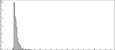
Figure 1: FADC traces of SD stations at 1 km from the shower core in units of VEM. Left: signal characteristic of a nearly vertical shower (zenith angle ${\sim}22^{\circ}$), where the electromagnetic component contributes about ${\sim}50$% to the total signal size. Right: signal characteristic of an inclined shower (zenith angle ${\sim}80^{\circ}$), where the muonic component dominates the total signal.

When shower electrons and photons ($\left\langle E\right\rangle\geq 10$ MeV) reach the surface detectors they are absorbed in the water and provide a Cherenkov light signal which is approximately proportional to the total deposited energy. Shower muons are more energetic ($E\geq 250$ MeV) and travel right through the tanks, typically giving signals proportional to their track length. For vertical showers initiated by protons or nuclei, the contribution of electrons and photons to the signal is often comparable or even larger than that due to the muons [15]. However, for inclined showers muons dominate the signal due to the electromagnetic component being largely absorbed by the atmosphere. Moreover the detector increases its relative response to muons with respect to electrons and photons as the zenith angle increases since the muon signal scales with the track length and the diameter of the tank exceeds its height.

The FD is distributed in four buildings on the perimeter of the surface array. Each building contains six telescopes that together cover $180^{\circ}$ in azimuth and nearly $30^{\circ}$ in elevation. The FD is fully described in [16]. Whereas the SD measurements are performed with a duty cycle of almost 100%, the FD only operates on clear moonless nights and has a duty cycle of 13%. The FD allows a calorimetric measurement of the shower energy deposited in the atmosphere, in contrast to the SD. The positions of the triggered pixels and the arrival time of the light are used to extract the shower direction. The profile function of the energy deposited in the atmosphere is determined from the signals at the triggered pixels [17] after taking into account the separate fluorescence and Cherenkov light contributions, as well as light attenuation and dispersion in the atmosphere. The atmospheric conditions are monitored regularly using several techniques to provide relevant data on attenuation and light dispersion parameters [18]. The electromagnetic energy released by the shower in the atmosphere is obtained by fitting the longitudinal profile to a Gaisser-Hillas function [19] and integrating over the range of atmospheric depths. The total energy of the primary particle is derived from the calorimetric energy by adding the invisible energy which accounts for the energy carried by penetrating particles. Most of the detected FD events also induce triggers of at least one SD station and are called hybrid events. The geometry of the shower axis can be determined more precisely for these events by using timing information from the FD pixels, coupled with the arrival time of the shower at the SD station with highest signal. A fraction of these hybrid events, called “golden hybrid” events, have sufficient SD stations triggered to allow for an independent reconstruction with SD techniques.

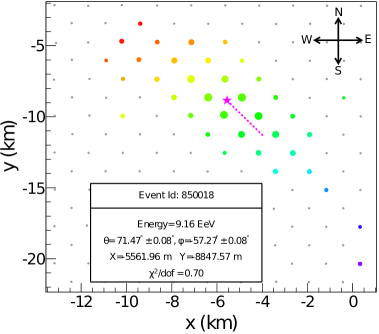
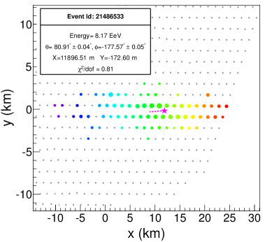
Figure 2: Inclined events with large number of triggered stations. The left (right) event with 37 (69) triggered stations corresponds to zenith angle $71^{\circ}$ ($81^{\circ}$) and azimuth angle to the East $-57^{\circ}$ ($-178^{\circ}$). The dashed line shows the shower axis projected onto the ground and the star indicates the core position. The areas of the circles are proportional to the logarithm of the signal size and the color code denotes the measured arrival time from early (blue) to late (red) stations.

2.1 Selection of inclined events with the Surface Detector

The SD trigger (described in detail in [20]) has been designed in a hierarchical pattern to identify a cosmic-ray event and reject random coincidences. The first two triggers, T1 and T2, apply at station level. T1 and T2 require that the pulse height of the signal exceeds two preset values (larger for T2 than for T1). Alternatively a second T2 trigger can also be obtained with smaller pulses that are spread in time (T2-ToT), which is a characteristic of the electromagnetic component in showers of near vertical incidence (see left panel of figure 1). The T1 trigger is stored temporarily while the data of all T2 triggers are sent to the central station. T2 triggered stations that lie in a close and compact configuration are checked for coincidences in time. If sufficient coincident stations are found, the third level trigger (T3) is passed and the acquisition process starts. In this process the T1 triggers stored at the local stations are also downloaded and added to the event.

Starting with the T3 triggers, a higher-level trigger hierarchy is implemented to satisfy the precision requirements of the consequent analysis. The T4 and T5 filters are respectively applied off-line for selecting physical events, and to ensure that they fall on a region of the array where the surface detectors were operational at the time of the event, to guarantee their quality. They are defined differently for inclined events. The “inclined T4” condition ensures that the start time of the signals of at least four nearby T2 triggered stations are compatible with a shower front moving at the speed of light. Accidental triggers are removed by eliminating stations that have times outside the window corresponding to the passage of the shower front, as determined by the rest of the stations. Stations are eliminated one by one (selecting the ones with the highest timing offsets) starting from the T3 trigger selection, until a satisfactory configuration with four or more stations in a compact arrangement is found. This removes a large number of showers reconstructed with incorrect arrival directions due to random coincidences. Events that have stations which are all aligned (according to the hexagonal pattern of the array) are excluded since the arrival direction cannot be reconstructed accurately from these start-time data.

The inclined T5 condition is defined so as to select events that fall inside a region of the array in which all stations were operational (“active”), requiring that the station that is nearest to the reconstructed core and its six adjacent stations are all operational. This active region defines an “active unit cell” shaped as a hexagon and forms the basis of the array aperture calculation [20]. The T5 condition serves two purposes: (i) it avoids the reconstruction of events that fall near to the edge of the array or in regions where a station is temporarily not fully operational, which can have large uncertainties, and (ii) it ensures that the shower falls inside the active area that has been considered to establish the aperture. Note that the T5 condition is the basic trigger of the selection criteria used for the subsequent analysis of inclined showers.

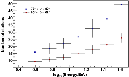
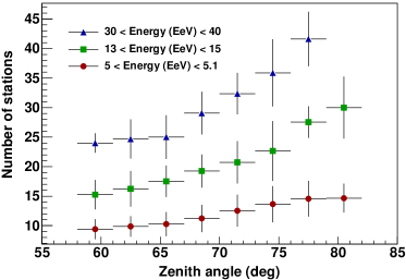
Figure 3: Left: average number of triggered stations as a function of shower energy. Right: the same as a function of the zenith angle. The vertical error bars correspond to the standard deviation of the number of stations.

2.2 General characteristics of inclined SD events

As the zenith angle $\theta$ of the showers increases, and they traverse larger atmospheric depths, the showers that reach the ground are increasingly attenuated. It appears that this would result in a reduced efficiency to detect inclined showers with the SD with increasing zenith angle. On the contrary, there is a compensating geometric effect since the density of stations in the shower plane (perpendicular to the shower axis) increases rapidly in proportion to $\sec\theta$. The signal reduction due to the muon attenuation over long path lengths is relatively small and is compensated by some of the surface detectors being closer to the shower axis where the signal is higher (compared to more vertical events) and thus more likely to trigger. Inclined events can have a large number of triggered stations as illustrated in figure 2.

This effect manifests itself when considering the number of triggered stations of events with a given energy as a function of zenith angle. For instance, considering an energy around 10 EeV (the energy at which the SD is fully efficient for events out to $80^{\circ}$), a vertical event has on average 8 triggered stations. This number is around 13 for a $60^{\circ}$ event of the same energy, while at $80^{\circ}$ it increases to 25. This effect is illustrated in figure 3 which shows the average number of stations as a function of shower energy at a fixed zenith angle (left panel) and the average number of stations as a function of zenith angle at a fixed energy (right panel).

3 Modeling particle distributions and detector responses

Showers with $\theta>60^{\circ}$ require specific reconstruction methods since they are dominated by muons displaying complex density patterns at the ground level. The method used for the reconstruction of inclined showers is based on a fit of the measured signals to the expected pattern, and requires modeling of a two-dimensional distribution of the muon number densities at the ground, the response of the detectors to the passage of muons, and the treatment of the electromagnetic component of the signal in the detectors.

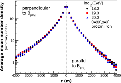
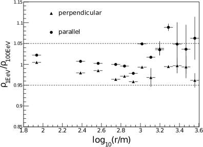
Figure 4: Left: average muon number density as a function of distance to the shower axis ($r$) in the shower plane, for showers with zenith angle $80^{\circ}$ and azimuth angle $0^{\circ}$ pointing to the East. The right (left) part of the $r$-axis corresponds to the direction parallel (perpendicular) to the projection of the geomagnetic field $\vec{B}$ onto the shower plane, $B_{\text{proj}}$. The distributions have been normalized to the equivalent density of $10^{19}$ eV to illustrate the degree to which the shapes are compatible, for three different energies and two primary compositions, as labeled. Right: ratio of average muon densities for 1 and 100 EeV proton showers, as a function of $r$ in the shower plane, after correction of the overall normalization.

3.1 Number density of muons at the ground

The number of muons per unit area, i.e. the muon density $\rho_{\mu}$, is a two dimensional function of position coordinates $(x,y)$ relative to the shower axis position $(x_{\text{c}},x_{\text{c}})$, that is $\vec{r}=(x-x_{\text{c}},y-y_{\text{c}})$, projected onto the shower plane. Descriptions of $\rho_{\mu}(\vec{r})$ at the ground level have been obtained and understood with the aid of comprehensive simulations of extensive air showers [3, 21].

As muons traverse the atmosphere they lose energy by ionization and hard muon interactions, namely bremsstrahlung, pair production and nuclear interactions via photo-nuclear processes. Below the critical energy for the muons, which is of order 500 GeV, ionization losses dominate. Decay probability in flight becomes important by effectively removing muons below an energy threshold which depends on both the muon energy and the distance traveled [22]. As the zenith angle increases from $60^{\circ}$ to $90^{\circ}$, the distance traveled to the ground level increases from ${\sim}10$ km to values over an order of magnitude larger, and the average energy of the muons at the ground level rises accordingly. The average energy of muons at the ground level, produced by a primary hadron at zenith angle $70^{\circ}$ ($80^{\circ}$), is about 25 (60) GeV.

In the Earth’s magnetic field $\vec{B}$, the muons are also deflected by the Lorentz force which laterally separates the positively and negatively charged muons [2]. Typical asymmetries are illustrated in Figs. 4 and 5. The separation proceeds in the direction perpendicular to the plane defined by the shower axis and the magnetic field. The magnitude of the separation depends mainly on the component of $\vec{B}$ perpendicular to the shower direction, the muon energy and the distance traveled [3]. The resulting signal patterns at the ground thus have a quite strong dependency on the arrival directions. As the zenith angle changes, the large variations in the distance traveled by the muons are to a large extent responsible for changes in the patterns at the ground level. As the azimuthal direction of the shower changes, smaller differences in the patterns are also observed, due to the varying angle between the typical muon velocity and the $\vec{B}$ field. Two different approaches have been used to obtain these distributions. One is based on a transformation of cylindrically symmetric patterns, exploiting the anti-correlation between muon energy and angle to the shower axis [3]. The other relies on continuous parameterizations in zenith angle and position in the shower plane that are fitted to results obtained from simulations [21]. Both approaches have been shown to reproduce the average profile of a given set of simulated showers with an accuracy better than 5%.

When the arrival direction and the nature of the primary particle are fixed, the muon number density has been shown to scale nearly linearly with shower energy ($\rho_{\mu}\propto E^{\alpha}$ with $\alpha$ typically being in the range $[0.90$–$0.95]$) [3, 21]. There are some differences between the distributions depending on the assumed nature of the primary particle, its energy and the hadronic interaction model used in the simulations. It has also been shown that these differences are manifested primarily by an overall normalization of the muon densities, and the shapes of these functions are approximately the same for a given arrival direction [23], i.e., weakly dependent on both shower energy and composition. Both characteristics are illustrated in figure 4.

The universal shape of the muon distribution and the scaling between muon number density and shower energy provide the basis of the fitting procedure. The reconstruction of the shower size is based on the fit of measured signals to the expected muon patterns. Details are fully described below.

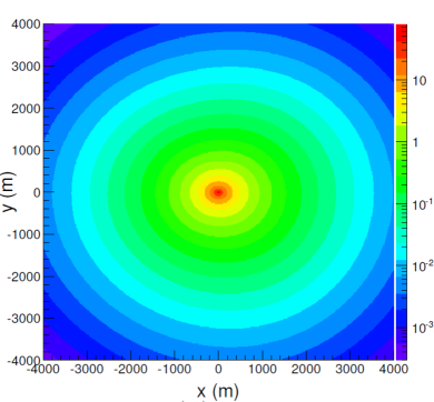
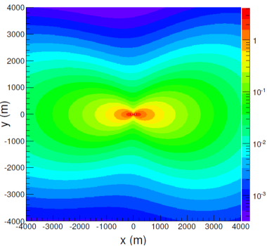
Figure 5: Contour plot of the muon density in the shower plane for $E=10$ EeV proton showers with zenith angles $70^{\circ}$ (left) and $84^{\circ}$ (right) and azimuth angle $0^{\circ}$, as obtained from simulations based on QGSJetII-03. The $y$-axis is oriented in the direction of the $\vec{B}$ field projected onto the shower plane.

According to the scaling property mentioned above, the expected muon number density at the ground can be written as:

$$\rho_{\mu}(\vec{r})=N_{19}\;\rho_{\mu,19}(\vec{r};\theta,\phi).$$ (3.1)

Here $N_{19}$ is a measure of the shower size and is the relative normalization of a particular event with respect to a reference muon distribution, $\rho_{\mu,19}(\vec{r};\theta,\phi)$, conventionally chosen to be the average muon density for primary protons with $E=10^{19}$ eV obtained with a chosen shower model, QGSJetII-03 [24] reference in our case. The dependence of these functions on the zenith and azimuth angles $(\theta,\phi)$ is indicated explicitly.

Two sets of muon distributions were generated for comparison purposes, one following [3] using the Aires [25] package for shower simulations with the QGSJet01 [26] model for hadronic interactions, and the other following [21] with Corsika [27] and QGSJetII-03. Examples of such distributions are shown in figure 5 for different zenith angles.

The actual value obtained for $N_{19}$ depends upon the particular choice of composition and hadronic model made for the reference distribution. The proton showers obtained with the QGSJetII-03 model was chosen as a reference for the data analysis presented in this work. For instance, the muon densities for proton showers derived using different high-energy hadronic interaction models scale with the approximate factors relative to the reference distribution given in table 1. A primary composition different from protons would also enhance the shower size scaling with the muon content [32]. In the extreme case of iron, the corresponding approximate factors are also given in table 1. These factors are indicative of the large expected uncertainties associated with the hadronic models and the unknown composition. Nevertheless, these uncertainties do not have a large impact on the measurement of the energy spectrum where the energy scale had been inferred from a sub-sample of events measured simultaneously with the FD and SD (see section 5). This analysis mimics the procedure to provide an absolute energy calibration [33] used for the reconstruction of events with zenith angle less than $60^{\circ}$. Most of the uncertainties associated with the unknown primary composition and hadronic model, as well as many uncertainties associated with the reconstruction, are absorbed in this robust and reliable calibration procedure.

Model	Proton	Iron
QGSJet01	1.10	1.46
QGSJetII-03	1.00	1.32
QGSJetII-04	1.19	1.58
Epos 1.99	1.25	1.65
Epos LHC	1.22	1.61
Sibyll 2.1	0.90	1.20

Table 1: Scale factors of the muon number densities derived for proton and iron showers simulated using different hadronic models [26, 24, 28, 29, 30, 31], relative to the reference muon distribution based on protons using QGSJetII-03.

3.2 Electromagnetic component

As inclined showers develop in the atmosphere, the EM cascade produced by the neutral pions in the hadronic collisions is attenuated, leaving a front dominated by muons. The remaining EM component (electrons, positrons and photons) originates from two different mechanisms. First is due to the tail of the hadronic cascade and decreases very rapidly as the zenith angle increases. Its magnitude depends on composition and interaction models. This component increases with the primary energy and varies according to the fluctuations in shower maximum. This dependence has to be considered as a source of systematic uncertainty in the electromagnetic correction, as will be discussed in section 4.2.3. The second component is produced by the muons themselves and closely follows the muon density patterns. It is mainly due to the showering of the electrons from muon decay in flight, although high-energy muons very close to the core also contribute through pair production and bremsstrahlung. More details can be found in [15].

In the reconstruction procedure (see section 4) the signals measured with the SD are compared to the reference muon distribution, and for this purpose it is necessary to extract the signal induced by muons from the total signal at each detector. This is achieved by subtracting the EM component from the detector signal using the average ratio, $R_{\text{EM}/\mu}(r,\theta)$, of the electromagnetic to the muonic contributions:

$$R_{\text{EM}/\mu}(r,\theta)=S_{\text{EM}}(r,\theta)/S_{\mu}(r,\theta).$$ (3.2)

This ratio was studied using Monte-Carlo simulations. Parameterizations of the average electromagnetic ($S_{\text{EM}}$) and muonic ($S_{\mu}$) contributions to the signal were obtained separately in terms of distance to the shower axis $r$, and of zenith angle $\theta$. Proton simulations at $10^{19}$ eV with QGSJet01 was chosen as a reference. The accuracy of this parameterization is better than 5%.

In figure 6 the ratio $R_{\text{EM}/\mu}$, averaged over the polar angle (with respect to the shower axis projected onto the shower plane), is shown as a function of $r$ for different $\theta$. The ratio can be seen to decrease as $\theta$ increases from ${\sim}60^{\circ}$ to $68^{\circ}$. At larger $\theta$ and near the shower axis, $R_{\text{EM}/\mu}$ can be seen to increase slightly due to hard muon interaction processes. At distances from the shower axis exceeding 1 km, $R_{\text{EM}/\mu}$ changes only weakly with distance, typically lying between 15% and 30%.

Figure 6: Ratio of the electromagnetic to muonic contributions to the detector signal averaged over the polar angle as a function of $r$, at different zenith angles.

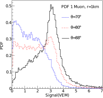
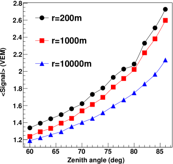
Figure 7: Left: probability distribution of the signal produced by single muons at a fixed distance of 1000 m from the shower axis, and for three different zenith angles. Right: average values of the signal produced by single muons as a function of zenith angle, for three different distances, as labeled.

3.3 Signal response of the surface detector stations

To reconstruct the position of the shower core and shower size $N_{19}$, the measured signals are fitted to the model predictions. The fit requires the evaluation of the probability density function (PDF) of the signal response of each surface detector to the expected number of muons. The PDF distributions are functions of the signal $S_{\mu}^{\text{meas}}$ deposited by muons in the detector, which is in turn estimated from the measured signal $S^{\text{meas}}$, using the average ratio of electromagnetic-to-muonic signals described in the previous section (eq. (3.2)):

$$S_{\mu}^{\text{meas}}=\frac{S^{\text{meas}}}{1+R_{\text{EM}/\mu}}.$$ (3.3)

The PDF for each surface detector is constructed from the expected number of muons, assuming Poisson statistics and using a simpler PDF corresponding to the passage of a fixed number of muons.

The basic prerequisite for these probability densities is the signal distribution for a detector hit by a single muon. These were obtained with high statistics using a module in the official software framework $\overline{\textrm{Off}}$ $\underline{\textrm{line}}$ [34] of the Pierre Auger Observatory, which simulates the detector response and interfaces it with the Geant4 package [35]. Multiple histograms for the signal response were generated for discrete values of $\theta$, and different relative positions of the station with respect to the shower core [36]. They are illustrated in Figs. 7 and 8. The signal is mainly due to the Cherenkov light emission by the muon tracks, and the PDF is closely related to the track-length distributions of the muons inside the detectors, which have a strong dependence on the zenith angle, as explicitly shown in figure 7.

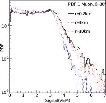
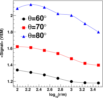
Figure 8: Left: probability distribution of the signal produced by single muons of $80^{\circ}$ and three different distances $r$ to shower core. Right: average signal produced by single muons as a function of $r$, for three zenith angles, as labeled.

The simulations include also contributions that do not scale with the muon track length and are dependent on the relative position of the stations. Delta rays (i.e., scattered electrons within the detector) account for an enhancement of the signal of order 20%, which increases with energy [4]. For high-energy muons bremsstrahlung, pair production and nuclear interactions inside the detector [4] give contributions which appear as harder tails of the response functions for stations close to the shower core. Low-energy muons have a reduced Cherenkov efficiency (enhanced by energy loss), becoming zero at the Cherenkov threshold. The average signal increases as the distance to the shower axis is reduced (as illustrated in figure 8) due to the increase in muon energy. The contribution, to the average signal, of the direct Cherenkov light that hits the photomultipliers without any reflection from the walls of the detector, ranges from 3% at $\theta=60^{\circ}$ to 10% at $80^{\circ}$.

Response histograms for single muons are used to obtain the response of the detector to the passage of multiple ($k$) muons by convolution in an iterative fashion, when $k$ is between 1 and 8. When $k>8$ a Gaussian approximation is used with an average $\xi_{k}=k\,\xi_{1}$ and a standard deviation of $\sigma_{k}=\sqrt{k}\,\sigma_{1}$, in terms of the averages ($\xi_{1}$) and standard deviations ($\sigma_{1}$) of the corresponding single muon histograms. As the number of muons grows, histograms rapidly become Gaussian-like, as anticipated from the Central Limit Theorem, see Fig 9. We label these PDF distributions as:

$$p_{\text{st}}(S_{\mu}^{\text{meas}};k,\vec{r},\theta),$$ (3.4)

explicitly indicating the dependence on $k$, $\theta$ and $\vec{r}$. The statistical uncertainty of these histograms is below $5\%$. A total of 12 960 histograms is needed to describe the signal distributions for the passage of $k$ muons ($k\,\leq\,8$) in 15 bins of $\theta$, 12 bins of polar angle and 9 bins of distance $r$.

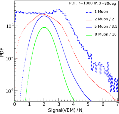
Figure 9: Probability distribution of the signal for a single muon with a zenith angle of $80^{\circ}$, falling 1000 m from the shower core, compared to the convolution for 2, 5 and 8 such muons. The distributions have been rescaled by a convenience factor given in labels.

4 Reconstruction

The reconstruction of inclined showers is performed first by fitting the arrival directions of the events using the start times of the signals, and then fitting the muon density patterns at the ground level to the signals measured by the surface detectors.

The reconstruction was also validated using large samples of simulated events. Extensive libraries of isotropically arriving proton and iron showers were made with a thinning level [37] of $10^{-6}$. A set of events simulated with Aires and QGSJet01 and a spectral index of $\gamma=2.6$ in the energy range $\log_{10}(E/\text{eV})=[18.5,20]$, and a zenith angle between $50^{\circ}$ and $89^{\circ}$ (100 000 events each) was used. A second and third set were simulated with Corsika using QGSJet-04 or Epos LHC, with a spectral index of $\gamma=1$ between $60^{\circ}$ and $89^{\circ}$. Each of these sets covers proton and iron in the same energy interval and is further split into three equal subintervals in $\log_{10}E$ (each energy subinterval has 30 000 events). Further libraries were also generated with QGSJetII-03 and Epos 1.99. All of these showers have subsequently undergone a full simulation of the detector with random impact points in the SD array, within the $\overline{\textrm{Off}}$ $\underline{\textrm{line}}$ framework, to generate databases of simulated events.

Unless otherwise indicated, the criteria used to select the simulated events for comparison match the selection that will be used for the measurement of the spectrum with inclined data. Events with $60^{\circ}<\theta<80^{\circ}$ are required to pass the inclined T4 and T5 conditions, with also $N_{19}>0.7$ to ensure the SD array is fully efficient.

4.1 Angular reconstruction

The directions of the incident cosmic rays are determined from the relative arrival times of the shower front in the triggered stations. The start times of the signals are fitted to those expected from a shower front with curvature, using a standard $\chi^{2}$ minimization procedure.

The angular accuracy depends on the number of triggered stations, on sizes of their signals, and also on the zenith angle of the shower itself. Typically, as the shower becomes more inclined, the arrival direction is reconstructed better, although this trend is inverted for events above $80^{\circ}$. As the shower becomes dominated by the muons, its front develops a smaller time spread than for vertical showers, and the start time can be established more precisely. In addition, as the zenith angle increases, the curvature of the shower front is reduced since the muons are produced further away from the ground and have higher energies. Finally, the number of triggered stations in a shower tends to increase as the zenith angle rises, due simply to the projection of the station positions into the shower plane.

Equivalent precision on angular reconstruction has been obtained with the different models used to describe the shower front and the variance reported in [22, 38].

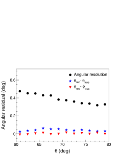
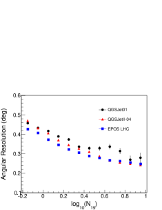
Figure 10: Comparison of reconstructed and true arrival directions with simulated events. Left: difference between true and reconstructed zenith (blue stars) and azimuth (red triangles) angles, as a function of the true zenith angle, for proton SD events simulated with QGSJet01. The angular resolution (black circles) is also shown. Right: angular resolution as a function of shower size for different hadronic models, QGSJet01 (black circles), QGSJetII-04 (red triangles) and Epos LHC (blue squares).

The angular reconstruction was tested with simulations. The left panel of figure 10 displays the difference between true and reconstructed angles, as well as the angular resolution as a function of zenith angle for showers simulated with QGSJet01 and for model [22]. The angular resolution, defined as the angle at 68% of the cumulative distribution function of the space angle (angular separation between the true and reconstructed directions), is obtained by fitting this distribution with a Gaussian resolution function, $\mathrm{d}p\propto\exp(-\alpha^{2}/2\sigma^{2})\,\mathrm{d}\cos\alpha\,\mathrm{d}\phi$, and corresponds to $1.5\times\sigma$ [39]. The right panel of figure 10 displays the angular resolution as a function of shower size, comparing the performance using different shower simulations and hadronic models. The reconstructed zenith and azimuth angles have a bias less than $0.08^{\circ}$ and $0.02^{\circ}$, respectively, and the angular resolution better than $0.5^{\circ}$, improving to better than $0.35^{\circ}$ for the highest energies.

The angular reconstruction of the SD was studied using hybrid data, data from a region of the array with stations on a 750 m grid, events with stations that are duplicated at given positions, and different samples of simulated SD events. These approaches have yielded compatible results.

4.2 Shower size and core position reconstruction

4.2.1 Procedure

Once the arrival direction is established, the expected number of muons $n_{\mu}$ at each station can be obtained multiplying the corresponding muon number density (eq. (3.1)) by the detector area $A_{\perp}$ projected onto the shower plane:

$$n_{\mu}=\rho_{\mu}(\vec{r})\;A_{\perp}(\theta)=N_{19}\;\rho_{\mu,19}(\vec{r};\theta,\phi)\;A_{\perp}(\theta).$$ (4.1)

Estimates of the position of the shower core $(x_{\text{c}},y_{\text{c}})$ and the shower size $N_{19}$ are obtained by fitting the expected number of muons $n_{\mu}$ to the muonic part of the measured signal $S_{\mu}^{\text{meas}}$ (eq. (3.3)). The fitting is performed using a maximum-likelihood method including the information from non-triggered and saturated stations. This constrains the shower size and reduces any selection bias due to the threshold trigger. The log-likelihood function is the logarithm of the combined probability $p$ to obtain the measured signals in all detectors. For each triggered and non-triggered participating station, this is taken as the product of the probability densities of getting the muonic signal $S_{\mu}^{\text{meas}}$ when $n_{\mu}$ muons are expected. Therefore, the log-likelihood function is given by:

$$\log\mathcal{L}=\sum_{i=1}^{N}\log p_{i}(S_{\mu}^{\text{meas}};n_{\mu},\vec{r},\theta)$$ (4.2)

and depends on the three free parameters which enter the calculation of $n_{\mu}$ (eq. (4.1)), two for the shower core position $(x_{\text{c}},y_{\text{c}})$ and one for the shower size $N_{19}$.

The measured signal $S_{\mu}^{\text{meas}}$ when $n_{\mu}$ muons are expected, can be produced by different number of muons $k$, each with different probability density function $p_{\text{st}}$ (see eq. (3.4) and figure 9). To compute each local probability $p$, the sum over all the probabilities $p_{\text{st}}$ for all possible numbers of muons $k$ to produce the measured signal has to be computed. Each probability must be weighted by the Poisson probability $\mathcal{P}_{\text{oisson}}(k;n_{\mu})$ of $k$ muons entering the station when $n_{\mu}$ are expected. Then, the overall probability of obtaining $S_{\mu}^{\text{meas}}$ in a given detector becomes:

$$p(S_{\mu}^{\text{meas}};n_{\mu},\vec{r},\theta)=P_{\text{tr}}(S^{\text{meas}})\,\sum_{k=1}^{\infty}\mathcal{P}_{\text{oisson}}(k;n_{\mu})\;p_{\text{st}}(S_{\mu}^{\text{meas}};k,\vec{r},\theta),$$ (4.3)

where the average trigger probability $P_{\text{tr}}(S^{\text{meas}})$ in terms of the signal at each station is also included. $P_{\text{tr}}(S^{\text{meas}})$, estimated using the signal distributions of the triggered stations in the data, is shown in figure 11.

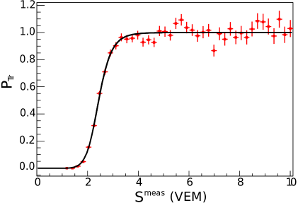
Figure 11: Estimate of the average probability that a detector triggers in terms of the measured signal.

The sum naturally accounts for Poisson fluctuations in the number of muons but additional signal fluctuations enter through $p_{\text{st}}$. The infinite sum is truncated for practical reasons.

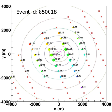
Figure 12: Left: display of a particular event projected onto the shower plane with the contour plot of the fitted distribution superimposed, indicating the signal measured in the 37 triggered stations and the position of the reconstructed core. The reconstructed zenith angle is $71^{\circ}$ and the best fit value of $N_{19}$ is 9.2 which corresponds to an energy of 54.6 EeV after the calibration procedure. The color code indicates the start time from early (blue) to late (red) stations. Right: signal sizes in the triggered stations as a function of the distance to the shower core in the shower plane for the same event. Filled and open symbols indicate measured and expected signals, respectively.

For stations that have no signal the probability distribution has to be replaced by the probability that the detector does not trigger. The probability that a station does not trigger can be obtained by integrating the detector response functions $p_{\text{st}}$, weighted by the probability function $1-P_{\text{tr}}(S^{\text{meas}})$ for not triggering. This is in turn obtained by summing the Poisson probabilities of having $k$ muons traversing the station, weighted by the corresponding probabilities for not triggering:

$$p(S_{\mu}^{\text{meas}}=0,n_{\mu};\vec{r},\theta)=\sum_{k=0}^{\infty}\mathcal{P}_{\text{oisson}}(k;n_{\mu})\int_{0}^{\infty}(1-P_{\text{tr}}(S))\,p_{\text{st}}(S;k,\vec{r},\theta)\,\mathrm{d}S.$$

To limit the computing time of the minimization procedure, only detector stations that have no signal and are within four concentric hexagons around all the triggered stations are included in the likelihood maximization procedure. For instance, the number of non-triggering stations entering the fit is on average ${\sim}8$ times the number of stations with signal. The number of stations without signal used for the reconstruction has a minor effect on the best fit value of $N_{19}$, and becomes negligible when sufficient stations have been considered. The average change in shower sizes when switching from four to two hexagons are below 5%.

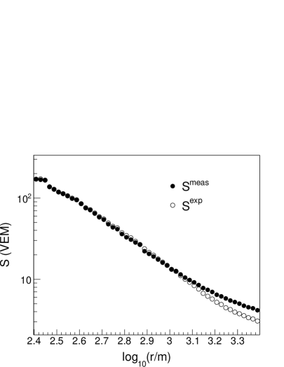
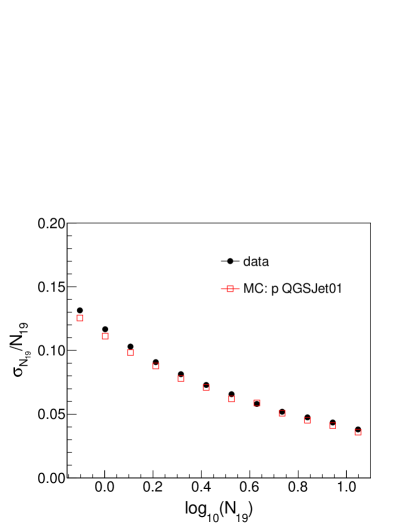
Figure 13: Left: signal size as a function of the distance to the shower core in the shower plane, for proton events simulated with QGSJet01. Filled and open symbols indicate measured and expected signals, respectively. Right: the average statistical relative uncertainty in $N_{19}$ as a function of $\log_{10}N_{19}$ for data and simulated events.

4.2.2 Performance

An example of a reconstructed event from the data is shown in the left panel of figure 12 indicating the position of the shower core and the contour plots of the average muon number density, in relation to the measured signals in the stations. The expected muon densities can be obtained by multiplying the density of the model distribution by the reconstructed value of $N_{19}$. The values of the expected and measured signals are shown in the right panel of figure 12 for the same event. For each triggered station, the expected muonic signal $S_{\mu}^{\text{exp}}$ is obtained by summing over all the average signal responses for all possible numbers of muons $k$ with Poisson weights, $\mathcal{P}_{\text{oisson}}(k;n_{\mu})$. Then, the expected signal $S^{\text{exp}}$ is estimated from $S_{\mu}^{\text{exp}}$ using the average ratio of electromagnetic and muonic signals: $S^{\text{exp}}=S_{\mu}^{\text{exp}}(1+R_{\text{EM}/\mu})$ (analogous to eq. (3.3)).

The performance is evaluated by studying the reconstruction of events obtained with full simulation. In the left panel of figure 13 the expected and measured signals are compared for a sample of simulated events. The reconstruction procedure achieves an agreement between expected and measured signals at the 5% level for expected signals above 10 VEM. Below this number, the comparison is not relevant due to the trigger effects and associated upward fluctuations of the signal. This is the reason why the “non-triggered” stations should be considered in the reconstruction, as explained in the previous section 4.2.1.

The reconstruction of the core position depends on the zenith angle, nevertheless this dependency is reduced when converted to the shower plane. The average distance between the reconstructed and true core positions in this plane is 108 m, ranging between 80 to 160 m as the zenith angle increases from $60^{\circ}$ to $80^{\circ}$.

The relative uncertainty in $N_{19}$ as obtained from the fit is shown in the right panel of figure 13 for data and simulated events. It decreases from about 13% at $N_{19}=0.7$ ($E=4$ EeV) to about $4\%$ at $N_{19}=10$ ($E=60$ EeV).

An approximate estimate of the true value of $N_{19}$ can be made for each simulated shower and compared to the reconstructed value. The number of muons $N_{\mu}$ that have reached the ground is obtained and normalized to the number of muons $N_{\mu,19}$ in the reference distribution (i.e. the integral of $\rho_{\mu,19}$ in eq. (3.1) over an area),

$$R_{\mu}=\frac{N_{\mu}}{N_{\mu,19}}.$$ (4.4)

The total number of muons in the reference distribution is shown in figure 14 where it is clear that the muon number is attenuated with the zenith angle, whereas, by definition, $N_{19}$ is independent of the zenith angle. The muon number is essentially independent of azimuth angle. For a given particle species and arrival direction the ratio, $R_{\mu}$, scales with shower energy, on average, and is normalized to $10^{19}$ eV, so that it can be compared directly with $N_{19}$.

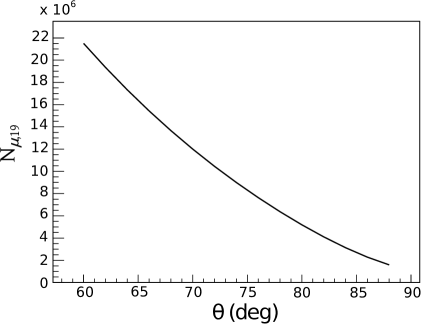
Figure 14: Total number of muons in the reference distribution as a function of the shower zenith angle. The reference distribution is based on proton showers with the energy of $10^{19}$ eV simulated using the QGSJetII-03 hadronic interaction model.

The difference between $N_{19}$ and $R_{\mu}$, and its standard deviation, are illustrated in the left and right panels of figure 15, respectively, for protons in a variety of models. The relative difference is on average less than 6%. This implies that $N_{19}$ is a good estimator of the number of muons in the shower. The relative difference observed can be interpreted as a bias in the measurement of the number of muons. It can be corrected for if $N_{19}$ is to be used as a measurement of the number of muons in the shower [40, 41]. However, such a bias has no relevance for the spectrum calculation, since the energy is finally obtained with the calibration procedure using events with their energy determined by the FD. The standard deviation decreases as the shower size increases, since for larger showers there are more stations entering the fit. Relative standard deviation ranges from 16 to 19% for the smaller shower sizes considered ($R_{\mu}\sim 0.7$) and drops to 5 to 9% for the largest events with $R_{\mu}>10$.

The presented standard deviation is an upper limit of the uncertainty of the fit to the muon distribution due to the shower-to-shower fluctuations. The shower-to-shower fluctuations imply variations in both the total number of muons and the shape of the muon distribution of a given shower with fixed arrival direction, energy and primary mass. If the showers only fluctuated by changing the scale of the muon distribution, the fitted value of $N_{19}$ would directly reflect the changes of normalization of the shower-to-shower fluctuations. But the fluctuations in the shape of the lateral profile are not taken into account in the fit which uses the average profile of the muon distribution. As a result, an unknown part of the shower-to-shower fluctuations propagates into the standard deviation shown in the right panel of figure 15. This is expected to be relatively small since the standard deviation at the larger shower sizes is well below the value of the fluctuations in $N_{\mu}$ for protons, which is about 20%.

In addition, the shown standard deviation includes the angular uncertainty propagated into $N_{19}$, nevertheless it has only a small effect. This is consistent with the uncertainties in $N_{19}$ obtained in the fitting procedure and shown in the right panel of figure 13.

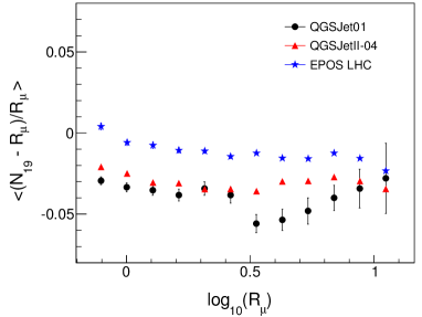
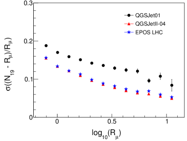
Figure 15: Mean (left) and standard deviation values (right) of the relative difference between $N_{19}$ and $R_{\mu}$ (see text), as a function of $R_{\mu}$ for simulated proton events.

The standard deviation is slightly lower (by ${\sim}3\%$) for showers simulated with QGSJetII-04 and Epos LHC than for those simulated with QGSJet01. This is possibly due to shower fluctuations and to the fact that the reference muon distributions were simulated with QGSJetII-03.

4.2.3 Systematic uncertainties

The EM correction to the detector signal (section 3.2) depends on the primary energy, on the composition and on the hadronic interaction model, and becomes largest in the reconstruction of shower size at zenith angles close to $60^{\circ}$. The actual value obtained for $N_{19}$ depends upon the particular choice of energy, composition and hadronic model made for the reference EM correction, which correspond to proton simulations at $10^{19}$ eV with QGSJet01 in this work. The systematic effect in $N_{19}$ associated with the unknown composition and the hadronic model was evaluated by computing alternative EM corrections (as defined in eq. (3.2)) with simulated showers using different combinations of energy ($10^{18}$ and $10^{20}$ eV), composition (proton and iron) and interaction models (QGSJet01 and Sibyll). A sample of data was reconstructed using these variations of the EM correction, leading to corresponding new values of the shower size, $N_{19}^{\text{corr}}$. The relative differences in shower size with respect to the reference provide estimates of the systematic uncertainties.

In figure 16 the relative differences for several scenarios are shown as a function of the shower zenith angle. The largest uncertainty in $N_{19}$ corresponds to the case of the correction computed with 100 EeV proton showers simulated with Sibyll. It decreases from 12% at $\theta\sim 60^{\circ}$ to less than 3% in absolute value at ${>}65^{\circ}$. This is a conservative estimate since it corresponds to an extreme situation in which the majority of data having energies of a few EeV are reconstructed with the electromagnetic correction corresponding to a 100 EeV shower.

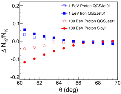
Figure 16: Systematic uncertainties in shower size of a data sample obtained by taking the difference between reconstructed values of $N_{19}$, using the default correction (10 EeV proton showers with QGSJet01), and alternative corrections derived from other simulations (as labeled). The energy dependence of the systematic effect is illustrated for 1 EeV (open squares) and 100 EeV (open circles) proton showers. Other scenarios are also shown for comparison (as labeled).

There can be other possible systematic effects on the shower size which depend on zenith angle and are not absorbed in the calibration procedure. Different hadronic interaction models and primary compositions may have different muon attenuations that is manifested in the zenith angle dependence of the muon distributions. These have an intrinsic dependence on the zenith angle which could in principle differ from that of the data. In addition, there are implicit uncertainties which can have zenith angle, dependence due to the accuracy of the models used for the muon distributions, the detector response and, most importantly, the electromagnetic correction.

The extent of these systematic uncertainties can be tested by exploring the zenith angle distribution of events above given thresholds of shower size. If the arrival directions are isotropically distributed and the detector has an efficiency that is independent of zenith angle $\theta$, the events should have a flat distribution in $\sin^{2}\theta$. Possible systematic effects associated with the zenith angle will appear as deviations from a uniform distribution. This test is quite sensitive due to the steeply falling spectrum. For a spectral index $\gamma$ it can be shown that a relative systematic shift of shower size $\Delta_{N_{19}}^{\text{sys}}/N_{19}$ in a given zenith angle bin should lead to a relative increase in the corresponding bin of ${\sim}(\gamma-1)\,\Delta_{N_{19}}^{\text{sys}}/N_{19}$.

Figure 17 displays the distribution of events with $N_{19}>1$ in bins of equal geometrical exposure. The array is fully efficient for showers of this size. The plot indicates that systematic deviations are within a 15% band with a standard deviation of ${\sim}8\%$. Assuming a spectral index $\gamma\simeq 2.69\pm 0.02$ as obtained with events below $60^{\circ}$, and for energies above 4 EeV [33] this systematic uncertainty corresponds to a potential shift in $N_{19}$ of less than $\pm 9\%$, well within the combined estimated uncertainties of the muon distributions, detector response and electromagnetic corrections.

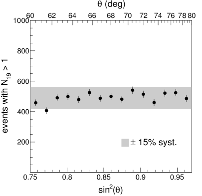
Figure 17: Distribution of data events with $N_{19}>1$ in $\sin^{2}\theta$ bins. A shaded band of 15% is shown to account for systematic uncertainties associated with the zenith angle in the models (see text).

5 Energy calibration and resolution

It is possible to relate $N_{19}$ to the shower energy using simulations, but due to the lack of knowledge of composition and hadronic models the corresponding systematic uncertainties become quite large (see section 3.1). Alternatively, the correlation between $N_{19}$ and shower energy reconstructed with the FD can be obtained from a subset of “golden hybrid” events (events for which both FD and SD reconstructions are possible), similarly to what has been used to calibrate events below $60^{\circ}$ [33]. The energy scale inferred from this subset is applied to all the inclined showers recorded with the SD.

The golden hybrid events with zenith angle greater than $60^{\circ}$ are required to pass the inclined T4 and T5 conditions and, in addition, to satisfy a set of FD quality cuts specifically designed to ensure an accurate reconstruction of the arrival direction and of the longitudinal profile. The cuts are adapted versions of those used in the calibration of events with $\theta<60^{\circ}$ [43]. The station closest to the shower core which is used for the geometrical reconstruction must be at a distance less than 750 m. For a precise estimate of the energy, we require an adequate monitoring of the atmospheric conditions (vertical aerosol optical depth up to 0.1; cloud coverage less than 25% in the FD field of view, distance of the cloud layer to the measured profile greater than 50 g/cm², and thickness of the cloud layer less than 100 g/cm²). Furthermore, we exclude a residual contamination of shower profiles distorted by clouds and aerosols by requiring a Gaisser-Hillas fit with a residual $(\chi^{2}-n_{\text{dof}})/\sqrt{2n_{\text{dof}}}$ smaller than 3 and a negative value of the parameter $X_{\text{0}}$ of the fitted Gaisser-Hillas profile. Moreover, the maximum accepted uncertainty of $X_{\text{max}}$ is 150 g/cm². In addition to the quality selection criteria, a fiducial cut on the FD field of view (FOV) is applied [46], ensuring that it is large enough to observe all plausible values of the shower maximum $X_{\text{max}}$. This “fiducial FOV cut” includes a restriction on the minimum viewing angle of the light in the FD telescope ($25^{\circ}$). Finally, only events with FD energies greater than $4{\times}10^{18}$ eV are accepted to ensure a trigger probability of nearly 100% for the SD and FD detectors. For the period from 1 January 2004 to 31 December 2012 the sample has 223 hybrid events with $\theta\geq 60^{\circ}$.

To describe the correlation it is sufficient to perform a power-law fit to the shower size $N_{19}$ as a function of the calorimetric hybrid energy $E_{\text{FD}}$,

$$N_{19}=A\,(E_{\text{FD}}/10^{19}\,\text{eV})^{B},$$ (5.1)

which is then inverted to give the energy conversion. The slope parameter $B$ is related to $\alpha$ ($\rho_{\mu}\propto E^{\alpha}$) as discussed in section 3.1. The fit must be handled with care since it is performed on a subset of the data used to calculate the spectrum. A bias can be expected at low energies due to the threshold trigger effects of the SD stations.

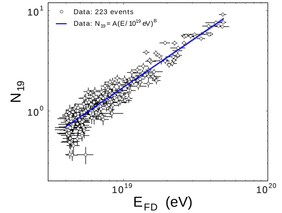
Figure 18: Correlation between $N_{19}$ and $E_{\text{FD}}$ for golden hybrid data with $\theta\geq 60^{\circ}$. The solid line is the best fit of the power-law $N_{19}=A\,(E_{\text{FD}}/10^{19}\,\text{eV})^{B}$ to the data (see text).

The fit is based on a tailored maximum-likelihood method [47] that takes into account the effect of the cut on energies greater than $4{\times}10^{18}$ eV, which would otherwise distort a standard least-squares fit. The ability to include both the uncertainties of the reconstructions of $N_{19}$ (see figure 13 in section 4.2.1) and $E_{\text{FD}}$, without relying on approximations, is another advantage of this approach. We achieve this by regarding the data as drawn from a two-dimensional probability density function $f(E_{\text{FD}},N_{19})$ that describes the random fluctuations away from the ideal curve given by eq. (5.1). The PDF is centered around this curve and its width is given by the uncertainties of the reconstructed values of $N_{19}$ and $E_{\text{FD}}$. Shower-to-shower fluctuations of $N_{19}$ also contribute to the spread and are taken into account. Their relative size is assumed to be constant in the energy range of interest and fitted to the data as an extra parameter. Since the data are described by a two-dimensional PDF, we are able to model the effect of an energy cut by setting the probability to observe events below the cut to zero. The effect of event migration in and out of the accepted region is also treated correctly. The method was validated with extensive Monte-Carlo studies and was found to fit the calibration curve without bias. The details will be presented in a dedicated article.

The result of this fit is illustrated in figure 18 and the best resulting parameters are $A=1.723\pm 0.023$ and $B=0.984\pm 0.020$. The calibration accuracy at the highest energies is limited by the number of events (the most energetic is at ${\sim}5{\times}10^{19}$ eV). An alternative fitting method based on least-squares minimization was used to calibrate the selected hybrid set as a cross-check. In this method the trigger bias is removed with an elliptical cut in the shower-size-energy plane to ensure that trigger effects can be ignored. The parameters obtained from the best fit are compatible with the maximum-likelihood fit.

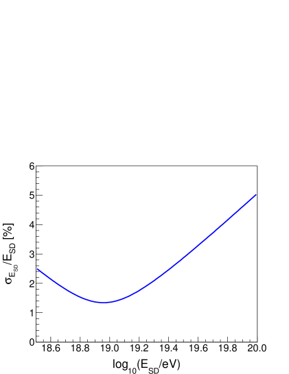
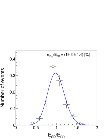
Figure 19: Left: relative systematic uncertainty in $E_{\text{SD}}$ as a function of shower energy as obtained by propagating the uncertainties from the correlation fit. Right: energy resolution inferred from the distribution of the ratio between calibrated SD energy $E_{\text{SD}}$ and FD energy $E_{\text{FD}}$ for all the golden hybrid data used in the calibration.

Eq. (5.1) can be used to convert $N_{19}$ to shower energy $E_{\text{SD}}$ for all the inclined events recorded with the SD. The statistical uncertainties of the calibration constants $A$ and $B$ were converted to uncertainties in $E_{\text{SD}}$ in the left panel of figure 19. The latter range between 1.5% at $10^{19}$ eV and 5% at $10^{20}$ eV.

To be detected with the FD the showers must have a depth of maximum well within the field of view, and to be detected with the SD the shower core must fall inside the array. The two simultaneous conditions suppress events with large zenith angles due to the geometrical layout of the Observatory [48]. The systematic uncertainty in $E_{\text{SD}}$, accounting for the different angular distributions of the golden hybrid events and the full inclined data set used to calculate the spectrum, is on average ${\sim}2\%$.

In addition, there is an overall systematic uncertainty of 14% from the FD energy measurement which relies on the knowledge of the fluorescence yield used in the energy determination of the FD events (3.6%), atmospheric conditions (3.4 to 6.2%), absolute detector calibration (9.9%), invisible energy (3 to 1.5%), stability of the energy scale (5%), and shower reconstruction (6.5 to 5.6%) [49].

The total systematic uncertainty in $E_{\text{SD}}$ ranges between 14% at $10^{19}$ eV and 17% at $10^{20}$ eV, and is obtained by adding the uncertainties described above in quadrature.

The right panel of figure 19 illustrates the ratio of the inferred SD energy $E_{\text{SD}}$ (after the calibration procedure) and the reconstructed FD-Hybrid energy $E_{\text{FD}}$. The resolution in the SD energy can be inferred from this ratio distribution [50], by fixing the FD energy resolution to 7.6% [49]. The resulting average SD energy resolution is $(19.3\pm 1.4)\%$ for the selected golden hybrid set. This SD energy resolution is attributed to the combined effect of shower-to-shower fluctuations and the reconstruction uncertainty of the fitting procedure (see figure 13 in section 4.2.1).

The fact that the value of the calibration parameter $A$ is not exactly equal to one reflects the fact that the signals detected with the SD are larger than expected from the reference distribution using protons. This is similar to the situation for events at zenith angles less than $60^{\circ}$, where the measured signal exceeds that expected for proton showers at the same energy, but the energy of the muons involved in inclined showers is significantly higher [3]. The obtained value of $A$ implies that $N_{19}=1$ corresponds to an FD energy of 5.75 EeV, about 42% less than the energy of 10 EeV used for the proton reference distributions. Equivalently, it implies that the number of muons in a 10 EeV shower is larger than the average muon content of the reference proton showers simulated with QGSJetII-03 [51]. This result has important implications concerning composition and hadronic models, which will be addressed in a separate article.

6 Summary and conclusions

We have developed a procedure to reconstruct inclined showers detected with the SD of the Pierre Auger Observatory. After reconstructing the arrival direction in a standard way using the start times of the recorded signals in the triggered stations, the signals of each event are fitted to the expected shape of the muon distribution at the ground. This requires modeling of the corresponding muon patterns, the response of the detectors to the passage of particles, and the amount of electromagnetic component of inclined showers, all of which were obtained with the aid of comprehensive simulations. The reference patterns for the muon distribution for each arrival direction are based on proton simulations with QGSJetII.03 at a fixed energy of 10 EeV. A size parameter $N_{19}$ has been introduced to scale the SD measurements to the reference distributions. $N_{19}$ is used as an energy estimator, calibrating it with the calorimetric energy measured by the FD, using a sub-sample of quality hybrid events which can be reconstructed independently using both the FD and SD techniques. In this process the simulated proton showers used to obtain the reference distributions of muons at the ground are shown to have a large deficit of muons with respect to the measured data.

The performance of the reconstruction was studied for events in the zenith angle range between $60^{\circ}$ and $80^{\circ}$, and with $N_{19}$ exceeding 0.7, to ensure nearly full efficiency for the trigger, selection and reconstruction of events that fall in active regions of the array. The angular resolution was shown to be better than $0.5^{\circ}$. The SD energy resolution was obtained, comparing the reconstructed SD and FD energies for the subset of events used in the energy calibration. The average SD energy resolution was shown to be about 19.3% attributed both to the reconstruction procedure and to the shower-to-shower fluctuations. Systematic uncertainties due to the calibration procedure were estimated to be energy dependent, and to fall in the range from 1.5 to 5%. In addition, there is an overall systematic uncertainty of 14% associated with the FD energy assignment. The procedure to analyze inclined events has a resolution in size and angular accuracy which is comparable to that obtained for events with $\theta<60^{\circ}$. The analysis of these events opens the possibility to measure the cosmic ray spectrum in an independent way, to explore primary composition, to study the fidelity of current hadronic models extrapolated to the high energies relevant to these events, and to analyze arrival directions from parts of the sky that are not accessible using events with zenith angles less than $60^{\circ}$. An independent measurement of the energy spectrum of ultra-high energy cosmic rays using very inclined showers is to be presented in a forthcoming publication.

References

- [1] Pierre Auger collaboration, J. Abraham et al., Properties and performance of the prototype instrument for the Pierre Auger Observatory, Nucl. Instrum. Meth. A 523 (2004) 50.
- [2] A. M. Hillas, in Proceedings of the 11 ICRC, Budapest, Hungry, Acta Phys. Acad. Sci. Hung. 29 (1970) 533.
- [3] M. Ave, R. A. Vazquez, and E. Zas, Modelling horizontal air showers induced by cosmic rays, Astropart. Phys. 14 (2000) 91 [astro-ph/0011490].
- [4] M. Ave, R. A. Vazquez, E. Zas, J. A. Hinton, and A. A. Watson, The rate of cosmic ray showers at large zenith angles: A step towards the detection of ultra-high energy neutrinos by the Pierre Auger Observatory, Astropart. Phys. 14 (2000) 109 [astro-ph/0003011].
- [5] V. M. Olmos Gilbaja, A Complete method to obtain the energy spectrum of inclined cosmic rays detected with the Pierre Auger Observatory (PhD thesis), University of Santiago de Compostela, Spain (2009).
- [6] H. Dembinski, Measurement of the ultra-high energy cosmic ray flux using data from very inclined air showers at the Pierre Auger Observatory (PhD thesis), RWTH Aachen University, Germany (2009).
- [7] R. A. Vazquez, for the Pierre Auger collaboration, The cosmic ray flux observed at zenith angles larger than with the Pierre Auger Observatory, in Proceedings of the 31 ICRC, Łódź, Poland (2009) [arXiv:0906.2189].
- [8] H. Dembinski, for the Pierre Auger collaboration, The cosmic ray spectrum above eV as measured with inclined showers recorded at the Pierre Auger Observatory, in Proceedings of the 32 ICRC, Beijing, China, 2 (2011) 101 [arXiv:1107.4809].
- [9] A. Schulz, for the Pierre Auger collaboration, The measurement of the energy spectrum of cosmic rays above eV with the Pierre Auger Observatory, in Proceedings of the 33 ICRC, Rio de Janeiro, Brasil (2013) [arXiv:1307.5059].
- [10] M. Ave, J. A. Hinton, R. A. Vazquez, A. A. Watson and E. Zas, New constraints from Haverah Park data on the photon and iron fluxes of UHE cosmic rays, Phys. Rev. Lett. 85 (2000) 2244 [astro-ph/0007386].
- [11] M. Ave, J. A. Hinton, R. A. Vazquez, A. A. Watson, and E. Zas, Sensitivity of the Auger Observatory to ultra high energy photon composition through inclined showers, Phys. Rev. D 67 (2003) 043005 [astro-ph/0208228].
- [12] V. S. Berezinsky and A. Y. .Smirnov, Cosmic neutrinos of ultra-high energies and detection possibility, Astrophys. Space Sci. 32 (1975) 461.
- [13] K. S. Capelle, J. W. Cronin, G. Parente and E. Zas, On the detection of ultrahigh-energy neutrinos with the Auger Observatory, Astropart. Phys. 8 (1998) 321 [astro-ph/9801313].
- [14] Pierre Auger collaboration, X. Bertou et al., Calibration of the surface array of the Pierre Auger Observatory, Nucl. Instrum. Meth. A 568 (2006) 839.
- [15] I. Valino, J. Alvarez-Muniz, M. Roth, R. A. Vazquez, and E. Zas, Characterisation of the electromagnetic component in ultra-high energy inclined air showers, Astropart. Phys. 32 (2010) 304 [arXiv:0910.2873].
- [16] Pierre Auger collaboration, J. Abraham et al., The Fluorescence Detector of the Pierre Auger Observatory, Nucl. Instrum. Meth. A 620 (2010) 227 [arXiv:0907.4282].
- [17] M. Unger, B. R. Dawson, R. Engel, F. Schussler, and R. Ulrich, Reconstruction of Longitudinal Profiles of Ultra-High Energy Cosmic Ray Showers from Fluorescence and Cherenkov Light Measurements, Nucl. Instrum. Meth. A 588 (2008) [arXiv:0801.4309].
- [18] Pierre Auger collaboration, J. Abraham et al., A Study of the Effect of Molecular and Aerosol Conditions in the Atmosphere on Air Fluorescence Measurements at the Pierre Auger Observatory, Astropart. Phys. 33 (2010) 108 [arXiv:1002.0366].
- [19] T. K.Gaisser and A. M. Hillas, Reliability of the method of constant intensity cuts for reconstructing the average development of vertical showers in Proceedings of the 15 ICRC, Plotdiv, Bulgaria, 8 (1977) 353.
- [20] Pierre Auger collaboration, J. Abraham et al., Trigger and aperture of the surface detector array of the Pierre Auger Observatory, Nucl. Instrum. Meth. A 613 (2010) 29 [arXiv:1111.6764].
- [21] H. P. Dembinski, P. Billoir, O. Deligny, and T. Hebbeker, A phenomenological model of the muon density profile on the ground of very inclined air showers, Astropart. Phys. 34 (2010) 128 [arXiv:0904.2372].
- [22] L. Cazon, R. A. Vazquez, A. A. Watson, and E. Zas, Time structure of muonic showers, Astropart. Phys. 21 (2004) 71 [astro-ph/0311223].
- [23] M. Ave, J. A. Hinton, R. A. Vazquez, A. A. Watson and E. Zas, Constraints on the ultrahigh-energy photon flux using inclined showers from the Haverah Park array, Phys. Rev. D 65 (2002) 063007 [astro-ph/0110613].
- [24] S. Ostapchenko, Non-linear screening effects in high energy hadronic interactions, Phys. Rev. D 74 (2006) 014026 [hep-ph/0505259].
- [25] S. J. Sciutto, The AIRES system for air shower simulations: An Update, in Proceedings of the 27 ICRC, Hamburg, Germany, 1 (2001) 237, (Copernicus Gesellschaft, Hamburg, 2001) [astro-ph/0106044].
- [26] N. N. Kalmykov and S. S. Ostapchenko, The Nucleus-nucleus interaction, nuclear fragmentation, and fluctuations of extensive air showers, Phys. Atom. Nucl. 56 (1993) 346 [Yad. Fiz. 56N3 (1993) 105]; N. N. Kalmykov, S. S. Ostapchenko and A. I. Pavlov, EAS and a quark - gluon string model with jets, Bull. Russ. Acad. Sci. Phys. 58 (1994) 1966 [Izv. Ross. Akad. Nauk Ser. Fiz. 58N12 (1994) 21].
- [27] D. Heck, G. Schatz, T. Thouw, J. Knapp and J. N. Capdevielle, CORSIKA: A Monte Carlo code to simulate extensive air showers, Report FZKA 6019, Forschungszentrum Karlsruhe, 1998.
- [28] S. Ostapchenko, Monte Carlo treatment of hadronic interactions in enhanced Pomeron scheme: I. QGSJET-II model, Phys. Rev. D 83 (2011) 014018 [arXiv:1010.1869].
- [29] T. Pierog and K. Werner, EPOS Model and Ultra High Energy Cosmic Rays, Nucl. Phys. Proc. Suppl. 196 (2009) 102–105 [arXiv:0905.1198].
- [30] T. Pierog, I. .Karpenko, J. M. Katzy, E. Yatsenko and K. Werner, EPOS LHC : test of collective hadronization with LHC data [arXiv:1306.0121].
- [31] R. Engel, T. K. Gaisser, P. Lipari, and T. Stanev, Nucleus-nucleus collisions and interpretation of cosmic-ray cascades Phys. Rev. D 46 (1992) 5013; R. S. Fletcher, T. K. Gaisser, P. Lipari, and T. Stanev, SIBILL: An event generator for simulation of high energy cosmic ray cascades, Phys. Rev. D 50 (1994) 5710.
- [32] M. Ave, J. A. Hinton, R. A. Vazquez, A. A. Watson and E. Zas, A New approach to inferring the mass composition of cosmic rays at energies above 10**18 eV, Astropart. Phys. 18 (2003) 367 [astro-ph/0112071].
- [33] Pierre Auger collaboration, J. Abraham et al., Observation of the suppression of the flux of cosmic rays above eV, Phys. Rev. Lett. 101 (2008) 061101 [arXiv:0806.4302].
- [34] S. Argiro, S. L. C. Barroso, J. Gonzalez, L. Nellen, T. C. Paul, T. A. Porter, L. Prado, Jr. and M. Roth et al., The Offline Software Framework of the Pierre Auger Observatory, Nucl. Instrum. Meth. A 580 (2007) 1485 [arXiv:0707.1652].
- [35] GEANT4 collaboration, S. Agostinelli et al., GEANT4: A Simulation toolkit, Nucl. Instrum. Meth. A 506 (2003) 250; J. Allison et al., Geant4 developments and applications, IEEE Trans. Nucl. Sci. 53 (2006) 270.
- [36] G. Rodríguez Fernández, Horizontal air showers at the Pierre Auger Observatory (PhD thesis), University of Santiago de Compostela, Spain (2007).
- [37] A. M. Hillas, in Proceedings of the 17 ICRC, Paris, France, 8 (1981) 193.
- [38] Pierre Auger collaboration, C. Bonifazi et al., A model for the time uncertainty measurements in the Auger surface detector array, Astropart. Phys. 28 (2008) 523 [arXiv:0705.1856].
- [39] Pierre Auger collaboration, C. Bonifazi, The angular resolution of the Pierre Auger Observatory, Nucl. Phys. Proc. Suppl. 190 (2009) 20 [arXiv:0901.3138].
- [40] I. Valiño, for the Pierre Auger collaboration, A measurement of the muon number in showers using inclined events recorded at the Pierre Auger Observatory, in Proceedings of the 33 ICRC, Rio de Janeiro, Brasil (2013) [arXiv:1307.5059].
- [41] Pierre Auger collaboration, A measurement of the muon number in showers using inclined events detected at the Pierre Auger Observatory, in preparation.
- [42] J. Alvarez-Muniz, R. Engel, T. K. Gaisser, J. A. Ortiz and T. Stanev, Atmospheric shower fluctuations and the constant intensity cut method, Phys. Rev. D 66 (2002) 123004 [astro-ph/0209117].
- [43] R. Pesce, for the Pierre Auger collaboration, Update of the energy calibration of data recorded with the surface detector of the Pierre Auger Observatory, in Proceedings of the 32 ICRC, Beijing, China, 2 (2011) 214 [arXiv:1107.4809].
- [44] C. Song, Longitudinal profile of extensive air showers, Astropart. Phys. 22 (2004) 151.
- [45] HIRES collaboration, T. Abu-Zayyad et al., A Measurement of the average longitudinal development profile of cosmic ray air showers between 10**17-eV and 10**18-eV, Astropart. Phys. 16 (2001) 1 [astro-ph/0008206].
- [46] Pierre Auger collaboration, J. Abraham et al., Measurement of the Depth of Maximum of Extensive Air Showers above 1018 eV, Phys. Rev. Lett. 104 (2010) 091101 [arXiv:1002.0699].
- [47] H. Dembinski, for the Pierre Auger collaboration, The cosmic ray spectrum above 4 EeV as measured with inclined showers recorded at the Pierre Auger Observatory, in Proceedings of the 32 ICRC, Beijing, China, 2 (2011) 101 [arXiv:1107.4804].
- [48] C. K. Guerard, for the Pierre Auger collaboration, Acceptance of the Pierre Auger Southern Observatory fluorescence detector to neutrino-like air showers, in Proceedings of the 27 ICRC, Hamburg, Germany, 1 (2001) 760, (Copernicus Gesellschaft, Hamburg, 2001).
- [49] V. Verzi, for the Pierre Auger collaboration, The Energy Scale of the Pierre Auger Observatory, in Proceedings of the 33 ICRC, Rio de Janeiro, Brasil (2013) [arXiv:1307.5059].
- [50] R. C. Geary, The frequency distribution of the quotient of two normal variates, J. R. Stat. Soc. 93 (1930) 442–446.
- [51] G. Rodriguez, for the Pierre Auger collaboration, Inclined showers at the Pierre Auger Observatory: reconstruction, energy calibration and implications for the muon content, in Proceedings of the 32 ICRC, Beijing, China, 2 (2011) 95 [arXiv:1107.4809].