Symbolic Algorithms for Language Equivalence
and Kleene Algebra with Tests

Abstract

We first propose algorithms for checking language equivalence of finite automata over a large alphabet. We use symbolic automata, where the transition function is compactly represented using a (multi-terminal) binary decision diagrams (BDD). The key idea consists in computing a bisimulation by exploring reachable pairs symbolically, so as to avoid redundancies. This idea can be combined with already existing optimisations, and we show in particular a nice integration with the disjoint sets forest data-structure from Hopcroft and Karp’s standard algorithm.

Then we consider Kleene algebra with tests (KAT), an algebraic theory that can be used for verification in various domains ranging from compiler optimisation to network programming analysis. This theory is decidable by reduction to language equivalence of automata on guarded strings, a particular kind of automata that have exponentially large alphabets. We propose several methods allowing to construct symbolic automata out of KAT expressions, based either on Brzozowski’s derivatives or standard automata constructions.

All in all, this results in efficient algorithms for deciding equivalence of KAT expressions.

1 Introduction

A wide range of algorithms in computer science build on the ability to check language equivalence or inclusion of finite automata. In model-checking for instance, one can build an automaton for a formula and an automaton for a model, and then check that the latter is included in the former. More advanced constructions need to build a sequence of automata by applying a transducer, and to stop whenever two subsequent automata recognise the same language Bouajjani et al. [2004]. Another field of application is that of various extensions of Kleene algebra, whose equational theories are reducible to language equivalence of various kinds automata: regular expressions and finite automata for plain Kleene algebra Kozen [1994], “closed” automata for Kleene algebra with converse Bloom et al. [1995]; Ésik and Bernátsky [1995], or guarded string automata for Kleene algebra with tests (KAT)

The theory of KAT has been developed by Kozen et al. Kozen [1997]; Cohen et al. [1996]; Kozen [2008], it has received much attention for its applications in various verification tasks ranging from compiler optimisation Kozen and Patron [2000] to program schematology Angus and Kozen [2001], and very recently for network programming analysis Anderson et al. [2014]; Foster et al. [2014]. Like for Kleene algebra, the equational theory of KAT is PSPACE-complete, making it a challenging task to provide algorithms that are computationally practical on as many inputs as possible.

One difficulty with KAT is that the underlying automata work on an input alphabet which is exponentially large in the number of variables of the starting expressions. As such, it renders standard algorithms for language equivalence intractable, even for reasonably small inputs. This difficulty is shared with other fields where various people proposed to work with symbolic automata to cope with large, or even infinite, alphabets Bryant [1992]; Veanes [2013]. By symbolic automata, we mean finite automata whose transition function is represented using a compact data-structure, typically binary decision diagrams (BDDs) Bryant [1986, 1992], allowing the explore the automata in a symbolic way.

D’Antoni and Veanes recently proposed a new minimisation algorithm for symbolic automata D’Antoni and Veanes [2014], which is much more efficient than the adaptations of the traditional algorithms Moore [1956]; Hopcroft [1971]; Paige and Tarjan [1987]. However, to our knowledge, the simpler problem of language equivalence for symbolic automata has not been covered yet. We say ‘simpler’ because language equivalence can be reduced trivially to minimisation—it suffices to minimise the automaton and to check whether the considered states are equated, but minimisation has complexity $n\mathrm{ln}n$ while Hopcroft and Karp’s algorithm for language equivalence Hopcroft and Karp [1971] is almost linear Tarjan [1975].

Our main contributions are the following:

• We propose a simple coinductive algorithm for checking language equivalence of symbolic automata (Section 3). This algorithm is generic enough to support various improvements that have been proposed in the literature for plain automata Wulf et al. [2006]; Abdulla et al. [2010]; Doyen and Raskin [2010]; Bonchi and Pous [2013].

• We show how to combine binary decisions diagrams (BDD) and disjoint set forests, the very elegant data-structure used by Hopcroft and Karp to defined their almost linear algorithm Hopcroft and Karp [1971]; Tarjan [1975] for deterministic automata. This results in a new version of their algorithm, for symbolic automata (Section 3.3).

• We study several constructions for building efficiently a symbolic automaton out of a KAT expression (Section 4): we consider a symbolic version of the extension of Brzozowski’s derivatives Brzozowski [1964] and Antimirov’ partial derivatives Antimirov [1996], as well as a generalisation of Ilie and Yu’s inductive construction Ilie and Yu [2003]. The latter construction also requires us to generalise the standard procedure consisting in eliminating epsilon transitions.

Notation

We denote sets by capital letters $X,Y,S,T\ldots$ and functions by lower case letters $f,g,\dots$ Given sets $X$ and $Y$, $X\times Y$ is their Cartesian product, $X\uplus Y$ is the disjoint union and $X^{Y}$ is the set of functions $f\colon Y\to X$. The collection of subsets of $X$ is denoted by ${\mathcal{P}}(()X)$. For a set of letters $A$, $A^{\star}$ denotes the set of all finite words over $A$; $\epsilon$ the empty word; and $w_{1}w_{2}$ the concatenation of words $w_{1},w_{2}\in A^{\star}$. We use $2$ for the set $\{0,1\}$.

2 Preliminary material

We first recall some standard definitions about finite automata and binary decision diagrams.

For finite automata, the only slight difference with the setting described in Bonchi and Pous [2013] is that we work with Moore machines Moore [1956] rather than automata: the accepting status of a state is not necessarily a Boolean, but a value in a fixed yet arbitrary set. Since this generalisation is harmless, we stick to the standard automata terminology.

2.1 Finite automata

A deterministic finite automaton (DFA) over the input alphabet $A$ and with outputs in $B$ is a triple $\langle S,t,o\rangle$, where $S$ is a finite set of states, $o\colon S\to B$ is the output function, and $t\colon S\to S^{A}$ is the transition function which returns, for each state $x$ and for each input letter $a\in A$, the next state $t_{a}(x)$. For $a\in A$, we write $x\stackrel{{\scriptstyle a}}{{\to}}x^{\prime}$ for $t_{a}(x)=x^{\prime}$. For $w\in A^{\star}$, we denote by $x\stackrel{{\scriptstyle w}}{{\to}}x^{\prime}$ for the least relation such that (1) $x\stackrel{{\scriptstyle\epsilon}}{{\to}}x$ and (2) $x\stackrel{{\scriptstyle aw^{\prime}}}{{\to}}x^{\prime}$ if $x\stackrel{{\scriptstyle a}}{{\to}}x^{\prime\prime}$ and $x^{\prime\prime}\stackrel{{\scriptstyle w^{\prime}}}{{\to}}x^{\prime}$.

The language accepted by a state $x\in S$ of a DFA is the function $\llbracket x\rrbracket\colon A^{\star}\to B$ defined as follows:

$$\llbracket x\rrbracket(\epsilon) =o(x)\enspace, \llbracket x\rrbracket(aw) =\llbracket t_{a}(x)\rrbracket(w)\enspace.$$

(When the output set is $2$, these functions are indeed characteristic functions of formal languages). Two states $x,y\in S$ are said to be language equivalent (written $x\sim y$) iff they accept the same language.

2.2 Coinduction

We then define bisimulations. We make explicit the underlying notion of progression which we need in the sequel.

Definition 1 (Progression, Bisimulation).

Given two relations $R,R^{\prime}\subseteq S\times S$ on states, $R$ progresses to $R^{\prime}$, denoted $R\rightarrowtail R^{\prime}$, if whenever $x\mathrel{R}y$ then

1. $o(x)=o(y)$ and

2. for all $a\in A$, $t_{a}(x)\mathrel{R^{\prime}}t_{a}(y)$.

A bisimulation is a relation $R$ such that $R\rightarrowtail R$.

Bisimulation is a sound and complete proof technique for checking language equivalence of DFA:

Proposition 1 (Coinduction).

Two states are language equivalent iff there exists a bisimulation that relates them.

Accordingly, we obtain the simple algorithm described in Figure 1, for checking language equivalence of two states of a given automaton. (Note that to check language equivalence of two states from two distinct automata, it suffices to consider the disjoint union of the two automata.)

⬇

1type ($s$,$\beta$) dfa = {t: $s$ $\to$ $A$ $\to$ $s$; o: $s$ $\to$ $\beta$}

2

3let equiv (M: ($s$,$\beta$) dfa) (x y: $s$) =

4 let r = Set.empty () in

5 let todo = Queue.singleton (x,y) in

6 while $\lnot$Queue.is_empty todo do

7 (* invariant: r \prog r \cup todo *)

8 let (x,y) = Queue.pop todo in

9 if Set.mem r (x,y) then continue

10 if M.o x $\neq$ M.o y then return false

11 iter_A (fun a $\to$ Queue.push todo (M.t x a, M.t y a))

12 Set.add r (x,y)

13 done;

14 return true

Figure 1: Simple algorithm for checking language equivalence.

This algorithm works as follows: the variable r contains a relation which is a bisimulation candidate and the variable todo contains a queue of pairs that remain to be processed. To process a pair $(x,y)$, one first checks whether it already belongs to the bisimulation candidate: in that case, the pair can be skipped since it was already processed. Otherwise, one checks that the outputs of the two states are the same ($o(x)=o(y)$), and one pushes all derivatives of the pair to the todo queue: all pairs $(t_{a}(x),t_{a}(y))$ for $a\in A$. The pair $(x,y)$ is finally added to the bisimulation candidate, and we proceed with the remainder of the queue.

The main invariant of the loop (line 7: $\mathtt{r}\rightarrowtail\mathtt{r}\cup\mathtt{todo}$) ensures that when todo becomes empty, then r contains a bisimulation, and the starting states were indeed bisimilar. Another invariant of the loop is that for any pair $(x^{\prime},y^{\prime})$ in todo, there exists a word $w$ such that $x\stackrel{{\scriptstyle w}}{{\to}}x^{\prime}$ and $y\stackrel{{\scriptstyle w}}{{\to}}y^{\prime}$. Therefore, if we reach a pair of states whose outputs are distinct—line 10, then the word $w$ associated to that pair witnesses the fact that the two initial states are not equivalent.

Remark 1.

Note that such an algorithm can be modified to check for language inclusion in a straightforward manner: assuming an arbitrary preorder $\leq$ on the output set $B$, and letting language inclusion mean $x\leq y$ if for all $w\in A^{\star}$, $\llbracket x\rrbracket(w)\leq\llbracket y\rrbracket(w)$, it suffices to replace line 10 in Figure 1 by

if $\lnot$(M.o x $\leq$ M.o y) then return false.

2.3 Up-to techniques

The previous algorithm can be enhanced by exploiting up-to techniques Sangiorgi [1998]; Pous and Sangiorgi [2011]: an up-to technique is a function $f$ on binary relations such that for any relation $R$ such that $R\rightarrowtail f(R)$ is contained in bisimilarity. Intuitively, such relations, that are not necessarily bisimulations, are constrained enough to be contained in bisimilarity.

Bonchi and Pous have recently shown Bonchi and Pous [2013] that the standard algorithm by Hopcroft and Karp Hopcroft and Karp [1971] actually exploits such an up-to technique: on line 9, rather than checking whether the processed pair is already in the candidate relation r, Hopcroft and Karp check whether it belongs to the equivalence closure of r. Indeed the function $e$ mapping a relation to its equivalence closure is a valid up-to technique, and this optimisation allows the algorithm to stop earlier. Hopcroft and Karp moreover use an efficient data-structure to perform this check in almost constant time Tarjan [1975]: disjoint sets forests. We recall this data-structure in Section 3.3.

Other examples of valid up-to techniques include context-closure, as used in antichain based algorithms Wulf et al. [2006]; Abdulla et al. [2010]; Doyen and Raskin [2010], or congruence closure Bonchi and Pous [2013], which combines both context-closure and equivalence closure. These techniques however require to work with automata whose state carry a semi-lattice structure, as is typically the case for a DFA obtained from a non-deterministic automaton, through the powerset construction.

2.4 Binary decision diagrams

Assume an ordered set $(A,<)$ and an arbitrary set $B$. Binary decision diagrams are directed acyclic graphs that can be used to represent functions of type $2^{A}\to B$. When $B=2$ is the two elements set, BDDs thus intuitively represent Boolean formulas with variables in $A$.

Formally, a (multi-terminal, ordered) binary decision diagram (BDD) is a pair $(N,c)$ where $N$ is a finite set of nodes and $c$ is a function of type $N\to B\uplus A\times N\times N$ such that if $c(n)=(a,l,r)$ and either $c(l)=(a^{\prime},\_,\_)$ or $c(r)=(a^{\prime},\_,\_)$, then $a<a^{\prime}$.

The condition on $c$ ensures that the underlying graph is acyclic, which make it possible to associate a function $\lceil n\rceil\colon 2^{A}\to B$ to each node $n$ of a BDD:

$$\lceil n\rceil(\alpha) =\begin{cases}b&\text{if }c(n)=b\in B\\ \lceil l\rceil(\alpha)&\text{if }c(n)=(a,l,r)\text{ and }\alpha(a)=0\\ \lceil r\rceil(\alpha)&\text{if }c(n)=(a,l,r)\text{ and }\alpha(a)=1\end{cases}$$

Let us now recall the standard graphical representation of BDDs:

• A node $n$ such that $c(n)=b\in B$ is represented by a square box labelled by $b$.

• A node $n$ such that $c(n)=(a,l,r)\in A\times N\times N$ is a decision node, which we picture by a circle labelled by $a$, with a dashed arrow towards the left child $(l)$ and a plain arrow towards the right child $(r)$.

For instance, the following drawing represents a BDD with three nodes; its top-most node denotes the function given on the right-hand side.

$$\alpha\mapsto\begin{cases}b_{1}&\text{if }\alpha(a_{1})=1\text{ and }\alpha(a_{2})=0\\ b_{2}&\text{otherwise}\end{cases}$$

A BDD is reduced if $c$ is injective, and $c(n)=(a,l,r)$ entails $l\neq r$. (The above example BDD is reduced.) Any BDD can be transformed into a reduced one. When $A$ is finite, reduced (ordered) BDD nodes are in one-to-one correspondence with functions from $2^{A}$ to $B$ Bryant [1986, 1992]. The main interest in this data-structure is that it is often extremely compact.

In the sequel, we only work with reduced ordered BDDs, which we simply call BDDs. We denote by $\mathrm{BDD}_{A}[B]$ the set of nodes of a large enough BDD with values in $B$, and we let $\lfloor f\rfloor$ denote the unique BDD node representing a given function $f\colon 2^{A}\to B$. This notation is useful to give abstract specifications to BDD operations: in the sequel, all usages of this notation actually underpin efficient BDD operations.

Implementation.

To better explain parts of the proposed algorithms, we give a simple implementation of BDDs in Figure 2.

⬇

1type $\beta$ node = $\beta$ descr hash_consed

2and $\beta$ descr = V of $\beta$ | N of $A$ $\times$ $\beta$ node $\times$ $\beta$ node

3

4val hashcons: $\beta$ descr $\to$ $\beta$ node

5val c: $\beta$ node $\to$ $\beta$ descr

6val memo_rec: (($\alpha$ $\to$ $\beta$ $\to$ $\gamma$) $\to$ $\alpha$ $\to$ $\beta$ $\to$ $\gamma$) $\to$ $\alpha$ $\to$ $\beta$ $\to$ $\gamma$

7

8let constant v = hashcons (V v)

9let node a l r = if l==r then l else hashcons (N(a,l,r))

10

11let apply (f: $\alpha$ $\to$ $\beta$ $\to$ $\gamma$): $\alpha$ node $\to$ $\beta$ node $\to$ $\gamma$ node =

12 memo_rec (fun app x y $\to$

13 match c(x), c(y) with

14 | V v, V w $\to$ constant (f v w)

15 | N(a,l,r), V _ $\to$ node a (app l y) (app r y)

16 | V _, N(a,l,r) $\to$ node a (app x l) (app x r)

17 | N(a,l,r), N(a’,l’,r’) $\to$

18 if a=a’ then node a (app l l’) (app r r’)

19 if a<a’ then node a (app l y ) (app r y )

20 if a>a’ then node a’ (app x l’) (app x r’))

Figure 2: An implementation of BDDs.

The type for BDD nodes is given first: we use Filliâtre’s hash-consing library Filliâtre and Conchon [2006] to enforce unique representation of each node, whence the two type declarations and the two conversion functions hashcons and c between those types. The third utility function memo_rec is just a convenient operator for defining recursive memoised functions.

The function constant creates a constant node, making sure it was not already created. The function node creates a new decision node, unless that node is useless and can be replaced by one of its two children. The generic function apply is central to BDDs Bryant [1986, 1992]: many operations are just instances of this function. Its specification is the following:

$$\mathtt{apply}~{}f~{}x~{}y =\lfloor\alpha\mapsto f(\lceil x\rceil(\alpha))(\lceil y\rceil(\alpha))\rfloor$$

This function is obtained by “zipping” the two BDDs together until a constant is reached. Memoisation is used to exploit sharing and to avoid performing the same computations again and again.

Suppose now that we want to define logical disjunction on Boolean BDD nodes. Its specification is the following:

$$x\lor y =\lfloor\alpha\mapsto\lceil n\rceil(\alpha)\lor\lceil m\rceil(\alpha)\rfloor.$$

We can thus simply use the apply function, applied to the Boolean disjunction function:

⬇

1let dsj: bool node $\to$ bool node $\to$ bool node = apply (||)

Note that this definition could actually be slightly optimised by inlining apply’s code, and noticing that the result is already known whenever one of the two arguments is a constant:

⬇

1let dsj: bool node $\to$ bool node $\to$ bool node =

2 memo_rec (fun dsj x y $\to$

3 match c(x), c(y) with

4 | V true, _ | _, V false $\to$ x

5 | _, V true | V false, _ $\to$ y

6 | N(a,l,r), N(a’,l’,r’) $\to$

7 if a=a’ then node a (dsj l l’) (dsj r r’)

8 if a<a’ then node a (dsj l y ) (dsj r y )

9 if a>a’ then node a’ (dsj x l’) (dsj x r’))

We ignore such optimisations in the sequel, for the sake of clarity.

3 Symbolic automata

A standard technique Bryant [1992]; Henriksen et al. [1995]; Veanes [2013]; D’Antoni and Veanes [2014] for working automata over a large input alphabet consists in using BBDs to represent the transition function: a symbolic DFA with output set $B$ and input alphabet $A^{\prime}=2^{A}$ for some set $A$ is a triple $\langle S,t,o\rangle$ where $S$ is the set of states, $t\colon S\to\mathrm{BDD}_{A}[S]$ maps states into nodes of a BDD over $A$ with values in $S$, and $o\colon S\to B$ is the output function.

Such a symbolic DFA is depicted in Figure 3. It has five states, input alphabet $2^{\{a,b,c\}}$, and natural numbers as output set. We represent the BDD graphically; for each state, we write the values of $t$ and $o$ together with the name of the state, in the corresponding square box. The explicit transition table is given below the drawing.

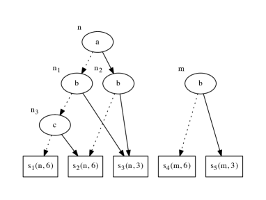
$$\begin{array}[]{c|l@{\,}l@{\,}l@{\,}l@{\,}l@{\,}l@{\,}l@{\,}l|l@{\,}l@{\,}l@{\,}l@{\,}l@{\,}l@{\,}l@{\,}l}&\lx@intercol\hfil s_{1},s_{2},s_{3}\hfil\lx@intercol&\lx@intercol\hfil s_{4},s_{5}\hfil\lx@intercol\\ \hline\cr a&0&0&0&0&1&1&1&1&0&0&0&0&1&1&1&1\\ b&0&0&1&1&0&0&1&1&0&0&1&1&0&0&1&1\\ c&0&1&0&1&0&1&0&1&0&1&0&1&0&1&0&1\\ \hline\cr t&s_{1}&s_{2}&s_{3}&s_{3}&s_{2}&s_{2}&s_{3}&s_{3}&s_{4}&s_{4}&s_{5}&s_{5}&s_{4}&s_{4}&s_{5}&s_{5}\\ \end{array}$$

Figure 3: A symbolic DFA with five states.

The simple algorithm described in Figure 1 is not optimal when working with such symbolic DFAs: at each non-trivial iteration of the main loop, one goes through all letters of $A^{\prime}=2^{A}$ to push all the derivatives of the current pair of states to the queue todo (line 11), resulting in a lot of redundancies.

Suppose for instance that we run the algorithm on the DFA of Figure 3, starting from states $s_{1}$ and $s_{4}$. After the first iteration, r contains the pair $(s_{1},s_{4})$, and the queue todo contains eight pairs:

$$(s_{1},s_{4}),(s_{2},s_{4}),(s_{3},s_{5}),(s_{3},s_{5}),(s_{2},s_{4}),(s_{2},s_{4}),(s_{3},s_{5}),(s_{3},s_{5})$$

Assume that elements of this queue are popped from left to right. The first two elements are removed during the next two iterations, since $(s_{1},s_{4})$ already is in r. Then $(s_{2},s_{4})$ is processed: it is added to r, and the above eight pairs are appended again to the queue, which now has thirteen elements. The following pair is processed similarly, resulting in a queue with twenty ($13-1+8$) pairs. Since all pairs of this queue are already in r, it is finally emptied through twenty iterations, and the algorithm returns true.

Note that it would be even worse if the input alphabet was actually declared to be $2^{\{a,b,c,d\}}$: even though the bit $d$ of all letters is irrelevant for the considered DFA, each non-trivial iteration of the algorithm would push even more copies of each pair to the todo queue.

What we propose here is to exploit the symbolic representation, so that a given pair is pushed only once. Intuitively, we want to recognise that starting from the pair of nodes $(n,m)$, the letters $010$, $011$, $110$ and $111$ are equivalent, since they yield to the same pair, $(s_{3},s_{5})$. Similarly, the letters $001$, $100$, and $101$ are equivalent: they yield to the pair $(s_{2},s_{4})$.

This idea is easy to implement using BDDs: like for the apply function (Figure 2), it suffices to zip the two BBDs together, and to push pairs when we reach two leaves. We use for that the procedure pairs from Figure 4, which successively applies a given function to all pairs reachable from two nodes. Its code is almost identical to apply, except that nothing is constructed (and memoisation is just used to remember those pairs that have already been visited).

⬇

1let pairs (f: $\alpha$ $\times$ $\beta$ $\to$ unit): $\alpha$ node $\to$ $\beta$ node $\to$ unit =

2 memo_rec (fun pairs x y $\to$

3 match c(x), c(y) with

4 | V v, V w $\to$ f (v,w)

5 | V _, N(_,l,r) $\to$ pairs x l; pairs x r

6 | N(_,l,r), V _ $\to$ pairs l y; pairs r y

7 | N(a,l,r), N(a’,l’,r’) $\to$

8 if a=a’ then pairs l l’; pairs r r’

9 if a<a’ then pairs l y ; pairs r y

10 if a>a’ then pairs x l’; pairs x r’)

Figure 4: Iterating over the set of pairs reachable from two nodes.

We finally modify the simple algorithm from Section 2.1 by using this procedure on line 11: we obtain the code given in Figure 5.

⬇

1type ($s$,$\beta$) sdfa = {t: $s$ $\to$ $s$ bdd; o: $s$ $\to$ $\beta$}

2

3let symb_equiv (M: ($s$,$\beta$) sdfa) (x y: $s$) =

4 let r = Set.empty () in

5 let todo = Queue.singleton (x,y) in

6 let push_pairs = pairs (Queue.push todo) in

7 while $\lnot$Queue.is_empty todo do

8 let (x,y) = Queue.pop todo in

9 if Set.mem r (x,y) then continue

10 if M.o x $\neq$ M.o y then return false

11 push_pairs (M.t x) (M.t y)

12 Set.add r (x,y)

13 done;

14 return true

Figure 5: Symbolic algorithm for checking language equivalence.

We apply pairs to its first argument once and for all (line 6), so that we maximise memoisation: a pair of nodes that has been visited in the past will never be visited again, since all pairs of states reachable from that pair of nodes is already guaranteed to be processed. (As an invariant, we have that all pairs reachable from a pair of nodes memoised in push_pairs appear in r \cup todo.)

Let us illustrate this algorithm by running it on the DFA from Figure 3, starting from states $s_{1}$ and $s_{4}$ as previously. During the first iteration, the pair $(s_{1},s_{4})$ is added to r, and push_pairs is called on the pair of nodes $(n,m)$. This call virtually results in building the following BDD,

so that the following three pairs are pushed to todo.

$$(s_{1},s_{4}),(s_{2},s_{4}),(s_{3},s_{5})$$

The first pair is removed by a trivial iteration: $(s_{1},s_{4})$ already belongs to r. The two other pairs are processed by adding them to r, but without pushing any new pair to todo: thanks to memoisation, the two expected calls to push_pairs n m are skipped.

All in all, each reachable pair is pushed only once to the todo queue. More importantly, the derivatives of a given pair are explored symbolically. In particular, the algorithm would execute exactly in the same way, even if the alphabet was actually declared to be much larger (for instance because the considered states were part of a bigger automaton with more letters).

3.1 Displaying symbolic counter-examples.

Another advantage of this new algorithm is that it can easily be instrumented to produce concise counter-examples in case of failure. Consider for instance the following automaton

Intuitively, the states $s_{1}$ and $s_{2}$ are not equivalent because $s_{2}$ can take three transitions to reach $s_{5}$, with output $1$, while $s_{1}$ cannot reach $s_{5}$ in three transitions.

More formally, the word $100~{}100~{}100$ over $2^{\{a,b,c\}}$ is a counter-example: we have

$$\llbracket s_{1}\rrbracket(100~{}100~{}100) =\llbracket s_{2}\rrbracket(100~{}100)=\llbracket s_{3}\rrbracket(100)=o(s_{4})=0$$

$$\llbracket s_{2}\rrbracket(100~{}100~{}100) =\llbracket s_{3}\rrbracket(100~{}100)=\llbracket s_{4}\rrbracket(100)=o(s_{5})=1$$

But there are plenty of other counter-examples of length three: it suffices that $a$ be assigned true in the three letters, the value of the bits $b$ and $c$ does not change the above computation. As a consequence, this counter-example is best described as the word $a\,a\,a$, whose letters are Boolean formulas in conjunctive normal form indicating the least requirements to get a counter example.

The algorithm from Figure 5 makes it possible to give this information back to the user:

• modify the queue todo to store triples $(w,x,y)$ where $(x,y)$ is a pair of states to process, and $w$ is the associated potential counter-example;

• modify the function pairs (Figure 4), so that it uses an additional argument to record the encountered node labels, with negative polarity when going through the recursive call for the left children, and positive polarity for the right children;

• modify line 10 of the main algorithm to return the symbolic word associated current pair when the output test fails.

3.2 Non-deterministic automata

Standard coinductive algorithms for DFA can be applied to non-deterministic automata (NFA) by using the powerset construction, on the fly. This construction transforms a non-deterministic automaton into a deterministic one; we extend it to symbolic automata in the straightforward way.

A symbolic NFA is a tuple $\langle S,t,o\rangle$ where $S$ is the set of states, $o\colon S\to B$ is the output function, and $t\colon S\to\mathrm{BDD}_{A}[{\mathcal{P}}(S)]$ maps a state and a letter of the alphabet $A^{\prime}=2^{A}$ to a set of possible successor states, using a symbolic representation.

Assuming such an NFA, one defines a symbolic DFA $\langle{\mathcal{P}}(S),t^{\sharp},o^{\sharp}\rangle$ as follows:

$$t^{\sharp}(\{x_{1},\dots,x_{n}\}) \triangleq t(x_{1})\mathrel{\underline{\cup}}\dots\mathrel{\underline{\cup}}t(x_{n})$$

$$o^{\sharp}(\{x_{1},\dots,x_{n}\}) \triangleq o(x_{1})\vee\dots\vee o(x_{n})$$

(Where $\mathrel{\underline{\cup}}$ denotes the pointwise union of two BDDs over sets: $n\mathrel{\underline{\cup}}m=\lfloor\phi\mapsto\lceil n\rceil(\phi)\cup\lceil m\rceil(\phi)\rfloor$.)

3.3 Hopcroft and Karp: disjoint sets forests

The previous algorithm can be freely enhanced by using up-to techniques, as described in Section 2.3: it suffices to modify line 9 to skip pairs more or less aggressively, according to the chosen up-to technique.

The up-to-equivalence technique used in Hopcroft and Karp’s algorithm can however be integrated in a deeper way, by exploiting the fact that we work with BDDs. This leads to a second algorithm, which we describe in this section.

Let us first recall disjoint sets forests, the data structure used by Hopcroft and Karp to represent equivalence classes. This standard data-structure makes it possible to check whether two elements belong to the same class and to merge two equivalence classes, both in almost constant amortised time Tarjan [1975].

The idea consists in storing a partial map from elements to elements and whose underlying graph is acyclic. An element for which the map is not defined is the representative of its equivalence class, and the representative of an element pointing in the map to some $y$ is the representative of $y$. Two elements are equivalent if and only if they lead to the same representative, and to merge two equivalence classes, it suffices to add a link from the representative of one class to the representative of the other class. Two optimisations are required to obtain the announced theoretical complexity:

• when following the path leading from an element to its representative, one should compress it in some way, by modifying the map so that the elements in this path become closer to their representative. There are various ways of compressing paths, in the sequel, we use the method called halving Tarjan [1975];

• when merging two classes, one should make the smallest one point to the biggest one, to avoid generating too many long paths. Again, there are several possible heuristics, but we elude this point in the sequel.

As explained above, the simplest thing to do would be to replace the bisimulation candidate $r$ from Figure 5 by a disjoint sets forest over the states of the considered automaton.

The new idea consists in relating the BBD nodes of the symbolic automaton rather that just its states (i.e., just the BDD leaves). By doing so, one avoids visiting pairs of nodes that have already been visited up to equivalence.

Concerning the implementation, we first introduce a variant of the function pair in Figure 6, which uses disjoint sets forest rather than plain memoisation.

⬇

1let pairs’ (f: $\beta$ $\times$ $\beta$ $\to$ unit): $\beta$ node $\to$ $\beta$ node $\to$ unit =

2 (* the disjoint sets forest *)

3 let m = Hmap.empty() in

4 let link x y = Hmap.add m x y in

5 (* representative of a node *)

6 let rec repr x =

7 match Hmap.get m x with

8 | None $\to$ x

9 | Some y $\to$ match Hmap.get m y with

10 | None $\to$ y

11 | Some z $\to$ link x z; repr z

12 in

13 let rec pairs x y =

14 let x = repr x in

15 let y = repr y in

16 if x $\neq$ y then

17 match c(x), c(y) with

18 | V v, V w $\to$ link x y; f (v,w)

19 | V _, N(_,l,r) $\to$ link y x; pairs x l; pairs x r

20 | N(_,l,r), V _ $\to$ link x y; pairs l y; pairs r y

21 | N(a,l,r), N(a’,l’,r’) $\to$

22 if a=a’ then link x y; pairs l l’; pairs r r’

23 if a<a’ then link x y; pairs l y ; pairs r y

24 if a>a’ then link y x; pairs x l’; pairs x r’)

25 in pairs

Figure 6: Iterating over the set of pairs reachable from two nodes, optimised using disjoint set forests.

This function first creates an empty forest (we use for that use Filliâtre’s implementation of maps over hash-consed values). The function link adds a link between two representatives; the recursive terminal function repr looks for the representative of a node and implements halving. The function pairs’ is defined similarly as pairs, except that it first takes the representative of the two given nodes, and that it adds a link from one to the other before recursing.

Those links can be put in any direction on lines 18 and 22, and we should actually use an appropriate heuristic to take this decision, as explained above. In the four other cases, we put a link either from the node to the leaf, or from the node with the smallest label to the node with the biggest label. By proceeding this way, we somehow optimise the BDD, by leaving as few decision nodes as possible.

It is however important to notice that there is actually no choice left in those four cases: we work implicitly with the optimised BDD obtained by mapping all nodes to their representatives, so that we have to maintain the invariant that this optimised BDD is ordered and acyclic. (Notice that on the contrary, this optimised BDD need not be reduced anymore: the children of given a node might be silently equated, and a node might have several representations since its children might be silently equated with the children of another node with the same label)

We finally obtain the algorithm given in Figure 7.

⬇

1let dsf_equiv (M: ($s$,$\beta$) sdfa) (x y: $s$) =

2 let todo = Queue.singleton (x,y) in

3 let push_pairs = pairs’ (Queue.push todo) in

4 while $\lnot$Queue.is_empty todo do

5 let (x,y) = Queue.pop todo in

6 if M.o x $\neq$ M.o y then return false

7 push_pairs (M.t x) (M.t y)

8 done;

9 return true

Figure 7: Symbolic algorithm optimised with disjoint set forests.

It is similar to the previous one (Figure 5), except that we use the above new function pairs’ to push pairs into the todo queue, and that we no longer need to store the bisimulation candidate r: this relation is subsumed by the restriction of the disjoint set forests to BDD leaves.

If we execute this algorithm on the symbolic DFA from Figure 3, between states $s_{1}$ and $s_{4}$, we obtain the disjoint set forest depicted below using dashed red arrows. This is actually corresponds to the pairs which would be visited by the first symbolic algorithm (Figure 5).

If instead we start from nodes $n1$ and $m1$ in the following partly described automaton, we would get the disjoint set forest depicted similarly in red, while the first algorithm would go through all blue pairs, one of which contains is superfluous.

4 Kleene algebra with tests

Now we consider Kleene algebra with tests, for which we provide several automata constructions that allow one to use the previous symbolic algorithms.

A Kleene algebra with tests (KAT) is a tuple $\langle X,B,{\cdot},{+},{\cdot^{\star}},\lnot,1,0\rangle$ such that

1. $\langle X,{\cdot},{+},{\cdot^{\star}},1,0\rangle$ is a Kleene algebra Kozen [1994], i.e., an idempotent semiring with a unary operation, called “Kleene star”, satisfying the following axiom and inference rules:

   $$1+x\cdot{}x^{\star}\leq x^{\star}\penalty 50\hskip 20.00003pt plus 0.5fil minus 5.0pt{\hbox{$\displaystyle\displaystyle{\hbox{\hskip 17.51266pt\vbox{\hbox{\hskip-17.51265pt\hbox{\hbox{$\displaystyle\displaystyle y\cdot{}x\leq x$}}}\vbox{}}}\over\hbox{\hskip 17.80157pt\vbox{\vbox{}\hbox{\hskip-17.80157pt\hbox{\hbox{$\displaystyle\displaystyle y^{\star}\cdot{}x\leq x$}}}}}}$}}\penalty 50\hskip 20.00003pt plus 0.5fil minus 5.0pt{\hbox{$\displaystyle\displaystyle{\hbox{\hskip 17.51266pt\vbox{\hbox{\hskip-17.51265pt\hbox{\hbox{$\displaystyle\displaystyle x\cdot{}y\leq x$}}}\vbox{}}}\over\hbox{\hskip 17.5238pt\vbox{\vbox{}\hbox{\hskip-17.5238pt\hbox{\hbox{$\displaystyle\displaystyle x\cdot{}y^{\star}\leq x$}}}}}}$}}$$

   (The preorder $(\leq)$ being defined by $x\leq y~{}\triangleq~{}x+y=y$.)

2. $B\subseteq X$

3. $\langle B,{\cdot},{+},{\neg},1,0\rangle$ is a Boolean algebra.

The elements of the set $B$ are called “tests”; we denote them by $\phi,\psi$. The elements of $X$, called “Kleene elements”, are denoted by $x,y,z$. We sometimes omit the operator “$\cdot$” from expressions, writing $xy$ for $x\cdot y$. The following (in)equations illustrate the kind of laws that hold in all Kleene algebra with tests:

$${}\phi+\neg\phi=1\penalty 50\hskip 20.00003pt plus 0.5fil minus 5.0pt\phi\cdot(\neg\phi+\psi)=\phi\cdot\psi=\neg(\neg\phi+\neg\psi)\penalty-10000\hskip 20.00003pt plus 0.5fil minus 5.0ptx^{\star}x^{\star}=x^{\star}\penalty 50\hskip 20.00003pt plus 0.5fil minus 5.0pt(x+y)^{\star}=x^{\star}(yx^{\star})^{\star}\penalty 50\hskip 20.00003pt plus 0.5fil minus 5.0pt(x+xxy)^{\star}\leq(x+xy)^{\star}\penalty-10000\hskip 20.00003pt plus 0.5fil minus 5.0pt\phi\cdot(\neg\phi\cdot x)^{\star}=\phi\penalty 50\hskip 20.00003pt plus 0.5fil minus 5.0pt\phi\cdot(\phi\cdot x\cdot\neg\phi+\neg\phi\cdot y\cdot\phi)^{\star}\cdot\phi\leq(x\cdot y)^{\star}$$

The laws from the first line come from the Boolean algebra structure, while the ones from the second line come from the Kleene algebra structure. The two laws from the last line require both Boolean algebra and Kleene algebra reasoning.

Binary relations.

Binary relations form a Kleene algebra with tests; this is the main model we are interested in, in practice. The Kleene elements are the binary relations over a given set $S$, the tests are the predicates over this set, encoded as sub-identity relations, and the star of a relation is its reflexive transitive closure.

This relational model is typically used to interpret imperative programs: such programs are state transformers, i.e., binary relations between states, and the conditions used to define the control-flow of these programs are just predicates on states. Typically, a program “while $\phi$ do p” is interpreted through the KAT expression $(\phi\cdot p)^{\star}\cdot\lnot\phi$.

KAT expressions.

We denote by $Rel(V)$ the set of regular expressions over a set $V$:

$$x,y::=v\in V\mid x+y\mid x\cdot y\mid x^{\star}\enspace.$$

Assuming a set $A$ of elementary tests, we denote by $B(A)$ the set of Boolean expressions over $A$:

$$\phi,\psi::=a\in A\mid 1\mid 0\mid\phi\land\phi\mid\phi\lor\phi\mid\lnot\phi$$

Further assuming a set $\Sigma$ of letters (or atomic Kleene elements), a KAT expression is a regular expression over the disjoint union $\Sigma\uplus B(A)$. Note that the constants $0$ and $1$ from the signature of KAT, and usually found in the syntax of regular expressions, are represented here by injecting the corresponding tests.

Guarded string languages.

Guarded string languages are the natural generalisation of string languages for Kleene algebra with tests. We briefly define them.

An atom is a valuation from elementary tests to Booleans; it indicates which of these tests are satisfied. We let $\alpha,\beta$ range over atoms, the set of which is denoted by $At$: $At=2^{A}$. A Boolean formula $\phi$ is valid under an atom $\alpha$, denoted by $\alpha\vDash\phi$, if $\phi$ evaluates to true under the valuation $\alpha$.

A guarded string is an alternating sequences of atoms and letters, both starting and ending with an atom:

$$\alpha_{1},p_{1},\alpha_{2},\dots,\alpha_{n},p_{n},\alpha_{n+1}\enspace.$$

The concatenation $u\ast v$ of two guarded strings $u,v$ is a partial operation: it is defined only if the last atom of $u$ is equal to the first atom of $v$; it consists in concatenating the two sequences and removing one copy of the shared atom in the middle.

To any KAT expression, one associates a guarded string language, i.e., a set of guarded strings, as follows:

$$G(\phi) =\{\alpha\in At\mid\alpha\vDash\phi\} (\phi\in B(A))$$

$$G(p) =\{\alpha p\beta\mid\alpha,\beta\in At\} (p\in\Sigma)$$

$$G(x+y) =G(x)\cup G(y)$$

$$G(xy) =\{u\ast v\mid u\in G(x),v\in G(y)\}$$

$$G(x^{\star}) =\{u_{1}\ast\dots\ast u_{n}\mid\exists u_{1}\dots u_{n},\forall i\leq n,u_{i}\in G(x)\}$$

KAT Completeness.

Kozen and Smith proved that the equational theory of Kleene algebra with tests is complete over the relational model Kozen and Smith [1996]: any equation that holds universally in this model can be proved from the axioms of KAT. Moreover, two expressions are provably equal if and only if they denote the same language of guarded strings. By a simple reduction to automata theory this gives algorithms to decide the equational theory of KAT. Now we study several such algorithms, and we show each time how to exploit symbolic representations to make them efficient.

4.1 Brzozowski’s derivatives

Derivatives were introduced by Brzozowski Brzozowski [1964] for (plain) regular expressions; they make it possible to define a deterministic automaton where the states of the automaton are the regular expressions themselves.

Derivatives can be extended to KAT expressions in a very natural way Kozen [2008]: we first define a Boolean function $\epsilon_{\alpha}$, that indicates whether an expression accepts the single atom $\alpha$; this function is then used to define the derivation function $\delta_{\alpha p}$, that intuitively returns what remains of the given expression after reading the atom $\alpha$ and the letter $p$.

$$\begin{aligned} \epsilon_{\alpha}(x{+}y)&=\epsilon_{\alpha}(x){+}\epsilon_{\alpha}(y)\\ \epsilon_{\alpha}(x{\cdot}y)&=\epsilon_{\alpha}(x){\cdot}\epsilon_{\alpha}(y)\\ \epsilon_{\alpha}(x^{\star})&=1\\ \epsilon_{\alpha}(q)&=0\\ \epsilon_{\alpha}(\phi)&=\begin{cases}1&\text{if }\alpha\vDash\phi\\ 0&\text{oth.}\end{cases}\end{aligned} \begin{aligned} \delta_{\alpha p}(x{+}y)&=\delta_{\alpha p}(x){+}\delta_{\alpha p}(y)\\ \delta_{\alpha p}(x{\cdot}y)&=\begin{cases}\delta_{\alpha p}(x){\cdot}y~{}\text{ if }\epsilon_{\alpha}(x)=0\\ \delta_{\alpha p}(x){\cdot}y{+}\delta_{\alpha p}(y)\text{ oth.}\end{cases}\\ \delta_{\alpha p}(x^{\star})&=\delta_{\alpha p}(x)\cdot x^{\star}\\ \delta_{\alpha p}(q)&=\begin{cases}1&\text{if }p=q\\ 0&\text{oth.}\end{cases}\\ \delta_{\alpha p}(\phi)&=0\end{aligned}$$

Figure 8: Explicit derivatives for KAT expressions

These two functions make it possible to give a coalgebraic characterisation of the function $G$, we have:

$$G(x)(\alpha) =\epsilon_{\alpha}(x) G(x)(\alpha\,p\,u) =G(\delta_{\alpha p}(x))(u)\enspace.$$

The tuple $\langle Reg(\Sigma\uplus B(A)),\delta,\epsilon\rangle$ can be seen as a deterministic automaton with input alphabet $At\times\Sigma$, and output set $2^{At}$. Thanks to the above characterisation, a state $x$ in this automaton accepts precisely the guarded string language $G(x)$—modulo the isomorphism $(At\times\Sigma)^{\star}\to 2^{At}\approx{\mathcal{P}}((At\times\Sigma)^{\star}\times At)$.

However, we cannot directly apply the simple algorithm from Section 2.1, because this automaton is not finite. First, there are infinitely many KAT expressions, so that we have to restrict to those that are accessible from the expressions we want to check for equality. This is however not sufficient: we also have to quotient regular expressions w.r.t. a few simple laws Kozen [2008]. This quotient is simple to implement by normalising expressions; we thus assume that expressions are normalised in the remainder of this section.

Symbolic derivatives.

The input alphabet of the above automaton is exponentially large w.r.t. the number of primitive tests: $At\times\Sigma=2^{A}\times\Sigma$. Therefore, the simple algorithm from Section 2.1 is not tractable in practice. Instead, we would like to use its symbolic version (Figure 5).

The output values (in $(2^{At}={2^{A}}\to 2)$) are also exponentially large, and are best represented symbolically, using Boolean BDDs. In fact, any test appearing in a KAT expression can be pre-compiled into a Boolean BDD: rather than working with regular expressions over $\Sigma\uplus B(A)$ we thus move to regular expressions over $\Sigma\uplus\mathrm{BDD}_{A}[2]$, which we call symbolic KAT expressions. We denote the set of such expressions by $\mathrm{SKAT}$, and we let $\llparenthesis e\rrparenthesis$ denote the symbolic version of a KAT expression $e$.

Note that there a slight discrepancy here w.r.t. Section 3: the input alphabet is $2^{A}\times\Sigma$ rather than just $2^{A^{\prime}}$ for some $A^{\prime}$. For the sake of simplicity, we just assume that $\Sigma$ is actually of the shape $2^{\Sigma^{\prime}}$; alternatively, we could work with automata whose transition functions are represented partly symbolically (for $At$), and partly explicitly (for $\Sigma$).

$$\begin{aligned} \epsilon^{\mathrm{s}}(x{+}y)&=\epsilon^{\mathrm{s}}(x){\vee}\epsilon^{\mathrm{s}}(y)\\ \epsilon^{\mathrm{s}}(x{\cdot}y)&=\epsilon^{\mathrm{s}}(x){\wedge}\epsilon^{\mathrm{s}}(y)\\ \epsilon^{\mathrm{s}}(x^{\star})&=1\\ \epsilon^{\mathrm{s}}(p)&=0\\ \epsilon^{\mathrm{s}}(\phi)&=\phi\end{aligned} \begin{aligned} \delta^{\mathrm{s}}(x{+}y)&=\delta^{\mathrm{s}}(x)\oplus\delta^{\mathrm{s}}(y)\\ \delta^{\mathrm{s}}(x{\cdot}y)&=(\delta^{\mathrm{s}}(x)\odot y)\oplus(\epsilon^{\mathrm{s}}(x)\otimes\delta^{\mathrm{s}}(y))\\ \delta^{\mathrm{s}}(x^{\star})&=\delta^{\mathrm{s}}(x)\odot x^{\star}\\ \delta^{\mathrm{s}}(p)&=\lceil p\mapsto 1,\_\mapsto 0\rceil\\ \delta^{\mathrm{s}}(\phi)&=0\end{aligned}$$

Figure 9: Symbolic derivatives for KAT expressions

We define the symbolic derivation operations in Figure 9.

The output function, $\epsilon^{\mathrm{s}}$, has type $\mathrm{SKAT}\to\mathrm{BDD}_{A}[2]$, it maps symbolic KAT expressions to Boolean BDD nodes. The operations used on the right-hand side of this definition are those on Boolean BDDs. The function $\epsilon^{\mathrm{s}}$ is much more efficient than its explicit counterpart ($\epsilon$, in Figure 8): the set of all accepted atoms is computed at once, symbolically.

The transition function $\delta^{\mathrm{s}}$, has type $\mathrm{SKAT}\to\mathrm{BDD}_{A\uplus\Sigma^{\prime}}[\mathrm{SKAT}]$. It maps symbolic KAT expressions to BDDs whose leaves are themselves symbolic KAT expressions. Again, in contrast to its explicit counterpart, $\delta^{\mathrm{s}}$ computes the all the transitions of a given expression once and for all. The operations used on the right-hand side of the definition are the following ones:

• $n\oplus m$ is defined by pointwise applying the syntactic sum operation from KAT expressions to the two BDDs $n$ and $m$: $n\oplus m=\lfloor\phi\mapsto\lceil n\rceil(\phi)+\lceil m\rceil(\phi)\rfloor$;

• $n\odot x$ syntactically multiplies all leaves of the BDD $n$ by the expression $x$, from the right: $n\odot x=\lfloor\phi\mapsto\lfloor n\rfloor(\phi)\cdot x\rfloor$;

• $f\otimes n$ “multiplies” the Boolean BDD $f$ with the BDD $n$: $f\otimes n=\lfloor\phi\mapsto\lfloor n\rfloor(\phi)\text{ if }\lfloor f\rfloor(\phi)=1,0\text{ otherwise}\rfloor$.

• $\lfloor q\mapsto 1,\_\mapsto 0\rfloor$ is the BDD mapping $q$ to $1$ and everything else to $0$ ($q\in\Sigma=2^{\Sigma^{\prime}}$ being casted into an element of $2^{A\uplus\Sigma^{\prime}}$).

By two simple inductions, one proves that for all atom $\alpha\in At$, expression $x\in\mathrm{SKAT}$, and letter $p\in\Sigma$, we have:

$$\lceil\epsilon^{\mathrm{s}}\llparenthesis x\rrparenthesis\rceil(\alpha) =\epsilon_{\alpha}(x)$$

$$\lceil\delta^{\mathrm{s}}\llparenthesis x\rrparenthesis\rceil(\alpha p) =\llparenthesis\delta_{\alpha p}(x)\rrparenthesis$$

(Again, we abuse notation by letting the pair $\alpha p$ denote an element of $2^{A\uplus\Sigma^{\prime}}$.) This ensures that the symbolic deterministic automaton $\langle\mathrm{SKAT},\delta^{\mathrm{s}},\epsilon^{\mathrm{s}}\rangle$ faithfully represents the previous explicit automaton, and that we can use the symbolic algorithms from Section 3.

4.2 Partial derivatives

An alternative to Brzozowski’s derivatives consists in using Antimirov’ partial derivatives Antimirov [1996], which generalise to KAT in a straightforward way Pous [2013]. The difference with Brzozowski’s derivative is that they produce a non-deterministic automaton: states are still expressions, but the derivation function produces a set of expressions. An advantage is that we do not need to normalise expressions: the set of partial derivatives reachable from an expression is always finite.

We give directly the symbolic definition, which is very similar to the previous one:

$$\delta^{{}^{\prime}\mathrm{s}}(x{+}y) =\delta^{{}^{\prime}\mathrm{s}}(x)\mathrel{\underline{\cup}}\delta^{{}^{\prime}\mathrm{s}}(y)$$

$$\delta^{{}^{\prime}\mathrm{s}}(x{\cdot}y) =(\delta^{{}^{\prime}\mathrm{s}}(x)\boxdot y)\mathrel{\underline{\cup}}(\epsilon^{\mathrm{s}}(x)\boxtimes\delta^{{}^{\prime}\mathrm{s}}(y))$$

$$\delta^{{}^{\prime}\mathrm{s}}(x^{\star}) =\delta^{{}^{\prime}\mathrm{s}}(x)\boxdot x^{\star}$$

$$\delta^{{}^{\prime}\mathrm{s}}(p) =\lfloor p\mapsto\{1\},\_\mapsto\emptyset\rfloor$$

$$\delta^{{}^{\prime}\mathrm{s}}(\phi) =\emptyset$$

The differences lie in the BDD operations, whose leaves are now sets of expressions:

• $n\mathrel{\underline{\cup}}m=\lfloor\phi\mapsto\lceil n\rceil(\phi)\cup\lceil m\rceil(\phi)\rfloor$;

• $n\boxdot x=\lfloor\phi\mapsto\{x^{\prime}\cdot x\mid x^{\prime}\in\lceil n\rceil(\phi)\}\rfloor$;

• $f\boxtimes n=\lfloor\phi\mapsto\lceil n\rceil(\phi)\text{ if }\lceil f\rceil(\phi)=1,\emptyset\text{ otherwise}\rfloor$.

One can finally relate partial derivatives to Brzozowski’s one:

$$\mathrm{KA}\vdash\Sigma_{x^{\prime}\in\delta^{\prime}_{\alpha p}(x)}x^{\prime}=\llparenthesis\delta_{\alpha p}(x)\rrparenthesis.$$

(We do not have a syntactic equality because partial derivatives inherently exploit the fact that multiplication distributes over sums.) Using symbolic determinisation as described in Section 3.2, one can thus use the algorithm from Section 3 with Antimirov’ partial derivatives.

4.3 Ilie & Yu’s construction

Other automata constructions from the literature can be generalised to KAT expressions. We can for instance consider Ilie and Yu’s construction Ilie and Yu [2003], which produces non-deterministic automata with epsilon transitions with exactly one initial state, and one accepting state.

We consider a slightly simplified version here, where we elude a few optimisations and just proceed by induction on the expression. The four cases are depicted below: $i$ and $f$ are the initial and accepting states, respectively; in the concatenation and star cases, a new state $p$ is introduced.

$$\phi/p: \textstyle{i} \scriptstyle{\phi/p} \textstyle{f} x\cdot y: \textstyle{i} \scriptstyle{A(x)} \textstyle{p} \scriptstyle{A(y)} \textstyle{f}$$

$$x+y: \textstyle{i} \scriptstyle{A(y)} \scriptstyle{A(x)} \textstyle{f} x^{\star}: \textstyle{i} \scriptstyle{1} \textstyle{p} \scriptstyle{1} \scriptstyle{A(x)} \textstyle{f}$$

To adapt this construction to KAT expressions, it suffices to generalise epsilon transitions to transitions labelled by tests. In the base case for a test $\phi$, we just add a transition labelled by $\phi$ between $i$ and $f$; the two epsilon transitions needed for the star case just become transitions labelled by the constant test $1$.

As expected, when starting from a symbolic KAT expression, those counterparts to epsilon transitions are labelled by Boolean BDD nodes rather than by explicit Boolean expressions.

Epsilon cycles.

The most important optimisation we miss with this simplified presentation of Ilie and Yu’s construction is that we should merge states that belong to cycles of epsilon transitions. An alternative to this optimisation consists in normalising first the expressions so that for all subexpressions of the shape $e^{\star}$, $e$ does not contain $1$, i.e., $\epsilon^{\mathrm{s}}(e)\neq 1$. Such a normalisation procedure has been proposed for plain regular expressions by Brüggemann-Klein Brüggemann-Klein [1993], it generalises easily to (symbolic) KAT expressions. For instance, here are typical normalisations:

$$(\phi+p)^{\star} \mapsto p^{\star}$$ (1)

$$(p^{\star}+q)^{\star} \mapsto(p+q)^{\star}$$ (2)

$$((1+p)(1+q))^{\star} \mapsto(p+q)^{\star}$$ (3)

When working with such normalised expressions, the automata produced by the above simplified construction have acyclic epsilon transitions, so that the aforementioned optimisation is unnecessary.

According to the example (1), it might be tempting to strengthen example (3) into $((\phi+p)(\psi+q))^{\star}\mapsto(p+q)^{\star}$. Such a step is invalid, unfortunately. (The second expression accepts the guarded string $\alpha p\beta$ for all $\alpha,\beta$, while the starting expression needs $\beta\vDash\psi$.) This example seems to show that one cannot ensure that all starred subexpressions are mapped to $0$ by $\epsilon^{\mathrm{s}}$. As a consequence we cannot assume that test-labelled transitions in general form an acyclic graph.

4.4 Epsilon transitions removal

It remains to eliminate epsilon transitions, so that the powerset construction can be applied to get a DFA. The usual technique with plain automata consists in computing the reflexive transitive closure of epsilon transitions, to precompose the other transitions with the resulting relation, and to saturate accepting states accordingly.

More formally, let us recall Kozen’s matricial representation of non-deterministic automaton with epsilon transitions Kozen [1994], as tuples $\langle n,u,J,N,v\rangle$, where $u$ is a $(1,n)$ 01-matrix denoting the initial states, $J$ is a $(n,n)$ 01-valued matrix denoting the epsilon transitions, $N$ is a $(n,n)$ matrix representing the other transitions (with entries sets of letters in $\Sigma$), and $v$ is a $(n,1)$ 01-matrix encoding the accepting states.

The language accepted by such an automaton can be represented by following the matricial product, using Kleene star on matrices:

$$u\cdot(J+N)^{\star}\cdot v$$

Thanks to the algebraic law $(a+b)^{\star}=a^{\star}\cdot(b\cdot a^{\star})^{\star}$, which is valid in any Kleene algebra, we get

$$KA\vdash u\cdot(J+N)^{\star}\cdot v=u\cdot(J^{\star}N)^{\star}\cdot(J^{\star}v)$$

We finally check that $\langle n,u,0,J^{\star}N,J^{\star}v\rangle$ represents a non-deterministic automaton without epsilon transitions. This is how Kozen validates epsilon elimination for plain automata, algebraically Kozen [1994].

The same can be done here for KAT by noticing that tests (or Boolean BDD nodes) form a Kleene algebra with a degenerate star operation: the constant-to-1 function. One can thus generalise the above reasoning to the case where $J$ is a tests-valued matrix rather than a 01-matrix.

The iteration $J^{\star}$ of such a matrix can be computed using standard shortest-path algorithms Höfner and Möller [2012], on top of the efficient semiring of Boolean BDD nodes. The resulting automaton has the expected type:

• there is a transition labelled by $\alpha p$ between $i$ and $j$ if there exists a $k$ such that $\alpha\vDash(J^{\star})_{i,k}$ and $p\in N_{k,j}$. (The corresponding non-deterministic symbolic transition function can be computed efficiently using appropriate BDD functions.)

• The output value of a state $i$ is the Boolean BDD node obtained by taking the disjunction of all the $(J^{\star})_{i,j}$ such that $j$ is an accepting state (i.e., just $(J^{\star})_{(i,f)}$ when using Ilie and Yu’s construction).

5 Experiments

We implemented all presented algorithms, the corresponding library is available online Pous [2014].

This allowed us to perform a few experiments and to compare the various presented algorithms and constructions. We generated random KAT expressions over two sets of seven primitive tests and seven atomic elements, with seventy connectives, and excluding the constant 0. A hundred pairs of random expressions were checked for equality after being saturated by adding the constant $\Sigma^{\star}$ (by doing so, we make sure that the expressions are equivalent, so that the algorithms have to run their worst case: they cannot stop early thanks to a trivial counter-example).

Table 1 gives the total number of output tests (e.g., line 10 in Figure 5) performed by several combinations of algorithms and automata constructions, as well as the global running time.

	symb_equiv			dsf_equiv
	Ant.	I.&Y.	Brz.	Ant.	I.&Y.	Brz.
time	1.5s	7.7s	2m34	1.4s	7.6s	1m52
output tests	7363	7440	20167	4322	4498	10255

Table 1: Checking random saturated pairs of expressions.

One can notice than Antimirov’ partial derivatives provide the fastest algorithms. Ilie and Yu’s construction yield approximately the same number of output tests as Antimirov’ partial derivatives, but require more time, certainly because our implementation of transitive closure for epsilon removal is sub-optimal. Brzozowski’s construction gives poor results both in terms of time and output tests: the produced automata are apparently larger, and heavier to compute.

Concerning the equivalence algorithm, one notices that using disjoint set forests significantly reduces the number of output tests. There is almost no difference in the timings with the first two constructions, because most of the time is spent in constructing the automata rather than checking them for equivalence. This is no longer true with Brzozowski’s construction, for which the automata are sufficiently big to observe a difference.

6 Directions for future work

Concerning KAT, a natural extension of this work would be to apply the proposed algorithms to KAT+!B Grathwohl et al. [2014] and NetKAT Anderson et al. [2014], two extensions of KAT with important applications in verification: while programs with mutable tests in the former case, and network programming in the later case.

KAT+!B has a EXPSPACE-complete equational theory, and its structure makes explicit algorithms completely useless. Designing symbolic algorithms for KAT+!B seems challenging.

NetKAT remains PSPACE-complete, and Foster et al. recently proposed a coalgebraic decision procedure relying on a extension of Brzozowski’s derivatives Foster et al. [2014]. To get a practical algorithm, they represent automata transitions using sparse matrices, which allows for some form of symbolic treatment. It is important to notice, however, that by considering (multi-terminal) BDDs here, we go far beyond the capabilities of sparse transition matrices. Indeed, sparse matrices just make it possible to factor out those cases where a state has no successor at all. Consider for instance a KAT expression of the shape $apx+(\lnot a)py$, where $x$ and $y$ are two non-empty expressions, possibly using a lot of atomic tests. The derivative of this expression along a letter $\alpha p$ is either $x$ or $y$ depending on whether $\alpha(a)$ holds or not. A BDD representation would thus consist in a single decision node, with two leaves $x$ and $y$. In contrast, a sparse matrix representation would need to list the exponentially many atoms together with either $x$ or $y$.

Moving away from KAT specificities, we leave open the question of the complexity of our symbolic variant of Hopcroft and Karp’s algorithm (Figure 7). Tarjan proved that Hopcroft and Karp’s algorithm is almost linear in amortised time complexity, and he made a list of heuristics and path compression schemes that lead to that complexity Tarjan [1975]. A similar study for the symbolic counterpart we propose here seems out of reach for now.

References

- Abdulla et al. [2010] P. A. Abdulla, Y.-F. Chen, L. Holík, R. Mayr, and T. Vojnar. When simulation meets antichains. In Proc. TACAS, volume 6015 of LNCS, pages 158–174. Springer, 2010.
- Anderson et al. [2014] C. J. Anderson, N. Foster, A. Guha, J.-B. Jeannin, D. Kozen, C. Schlesinger, and D. Walker. Netkat: semantic foundations for networks. In POPL, pages 113–126. ACM, 2014.
- Angus and Kozen [2001] A. Angus and D. Kozen. Kleene algebra with tests and program schematology. Technical Report TR2001-1844, CS Dpt, Cornell University, July 2001.
- Antimirov [1996] V. M. Antimirov. Partial derivatives of regular expressions and finite automaton constructions. TCS, 155(2):291–319, 1996.
- Bloom et al. [1995] S. L. Bloom, Z. Ésik, and G. Stefanescu. Notes on equational theories of relations. Algebra Universalis, 33(1):98–126, 1995.
- Bonchi and Pous [2013] F. Bonchi and D. Pous. Checking nfa equivalence with bisimulations up to congruence. In Proc. POPL, pages 457–468. ACM, 2013. ISBN 978-1-4503-1832-7.
- Bouajjani et al. [2004] A. Bouajjani, P. Habermehl, and T. Vojnar. Abstract regular model checking. In Proc. CAV, volume 3114 of LNCS, pages 372–386. Springer, 2004.
- Brüggemann-Klein [1993] A. Brüggemann-Klein. Regular expressions into finite automata. TCS, 120(2):197–213, 1993. http://dx.doi.org/10.1016/0304-3975(93)90287-4.
- Bryant [1986] R. E. Bryant. Graph-based algorithms for boolean function manipulation. IEEE Trans. Computers, 35(8):677–691, 1986.
- Bryant [1992] R. E. Bryant. Symbolic boolean manipulation with ordered binary-decision diagrams. ACM Comput. Surv., 24(3):293–318, 1992.
- Brzozowski [1964] J. A. Brzozowski. Derivatives of regular expressions. J. ACM, 11(4):481–494, 1964.
- Cohen et al. [1996] E. Cohen, D. Kozen, and F. Smith. The complexity of Kleene algebra with tests, 1996. TR96-1598, CS Dpt., Cornell University.
- D’Antoni and Veanes [2014] L. D’Antoni and M. Veanes. Minimization of symbolic automata. In POPL, pages 541–554. ACM, 2014.
- Doyen and Raskin [2010] L. Doyen and J.-F. Raskin. Antichain Algorithms for Finite Automata. In Proc. TACAS, volume 6015 of LNCS. Springer, 2010.
- Ésik and Bernátsky [1995] Z. Ésik and L. Bernátsky. Equational properties of Kleene algebras of relations with conversion. TCS, 137(2):237–251, 1995.
- Filliâtre and Conchon [2006] J.-C. Filliâtre and S. Conchon. Type-safe modular hash-consing. In ML, pages 12–19. ACM, 2006.
- Foster et al. [2014] N. Foster, D. Kozen, M. Milano, A. Silva, and L. Thompson. A coalgebraic decision procedure for NetKAT. Technical Report http://hdl.handle.net/1813/36255, Computing and Information Science, Cornell University, March 2014.
- Grathwohl et al. [2014] N. B. B. Grathwohl, D. Kozen, and K. Mamouras. KAT + B! Technical Report http://hdl.handle.net/1813/34898, Computing and Information Science, Cornell University, January 2014. To appear in Proc. CSL-LICS’14.
- Henriksen et al. [1995] J. G. Henriksen, J. L. Jensen, M. E. Jørgensen, N. Klarlund, R. Paige, T. Rauhe, and A. Sandholm. Mona: Monadic second-order logic in practice. In TACAS, volume 1019 of LNCS, pages 89–110. Springer, 1995.
- Höfner and Möller [2012] P. Höfner and B. Möller. Dijkstra, floyd and warshall meet kleene. Formal Asp. Comput., 24(4-6):459–476, 2012.
- Hopcroft [1971] J. E. Hopcroft. An algorithm for minimizing states in a finite automaton. Technical report, Stanford University, 1971.
- Hopcroft and Karp [1971] J. E. Hopcroft and R. M. Karp. A linear algorithm for testing equivalence of finite automata. Technical Report 114, Cornell University, December 1971.
- Ilie and Yu [2003] L. Ilie and S. Yu. Follow automata. Inf. and Comp., 186(1):140–162, 2003.
- Kozen [1994] D. Kozen. A completeness theorem for Kleene algebras and the algebra of regular events. Inf. and Comp., 110(2):366–390, 1994.
- Kozen [1997] D. Kozen. Kleene algebra with tests. Transactions on Programming Languages and Systems, 19(3):427–443, May 1997.
- Kozen [2008] D. Kozen. On the coalgebraic theory of Kleene algebra with tests. Technical Report http://hdl.handle.net/1813/10173, CIS, Cornell University, March 2008.
- Kozen and Patron [2000] D. Kozen and M.-C. Patron. Certification of compiler optimizations using Kleene algebra with tests. In Proc. CL2000, volume 1861 of LNAI, pages 568–582. Springer, 2000.
- Kozen and Smith [1996] D. Kozen and F. Smith. Kleene algebra with tests: Completeness and decidability. In Proc. CSL, volume 1258 of LNCS, pages 244–259. Springer, September 1996.
- Moore [1956] E. F. Moore. Gedanken-experiments on sequential machines. Automata Studies, Annals of Mathematical Studies, 34:129–153, 1956.
- Paige and Tarjan [1987] R. Paige and R. E. Tarjan. Three partition refinement algorithms. SIAM J. Comput., 16(6):973–989, 1987.
- Pous [2013] D. Pous. Kleene Algebra with Tests and Coq tools for while programs. In Proc. ITP, volume 7998 of LNCS, pages 180–196. Springer, 2013.
- Pous [2014] D. Pous. Web appendix to this paper, with Ocaml implementation of the proposed algorithms, 2014. URL http://perso.ens-lyon.fr/damien.pous/symbolickat.
- Pous and Sangiorgi [2011] D. Pous and D. Sangiorgi. Advanced Topics in Bisimulation and Coinduction, chapter about “Enhancements of the coinductive proof method”. CUP, 2011. ISBN 9781107004979.
- Sangiorgi [1998] D. Sangiorgi. On the bisimulation proof method. MSCS, 8:447–479, 1998.
- Tarjan [1975] R. E. Tarjan. Efficiency of a good but not linear set union algorithm. J. ACM, 22(2):215–225, 1975.
- Veanes [2013] M. Veanes. Applications of symbolic finite automata. In CIAA, volume 7982 of LNCS, pages 16–23. Springer, 2013.
- Wulf et al. [2006] M. D. Wulf, L. Doyen, T. A. Henzinger, and J.-F. Raskin. Antichains: A new algorithm for checking universality of finite automata. In Proc. CAV, volume 4144 of LNCS, pages 17–30. Springer, 2006.