Quasiparticle breakdown in the quasi-one-dimensional Ising ferromagnet CoNb₂O₆

Abstract

We present experimental and theoretical evidence that an interesting quantum many-body effect – quasi-particle breakdown – occurs in the quasi-one-dimensional spin-$\frac{1}{2}$ Ising-like ferromagnet ${\rm CoNb}_{2}{\rm O}_{6}$ in its paramagnetic phase at high transverse field as a result of explicit breaking of spin inversion symmetry. We propose a quantum spin Hamiltonian capturing the essential one-dimensional physics of ${\rm CoNb}_{2}{\rm O}_{6}$ and determine the exchange parameters of this model by fitting the calculated single particle dispersion to the one observed experimentally in applied transverse magnetic fieldsCabrera et al. (2014). We present high-resolution inelastic neutron scattering measurements of the single particle dispersion which observe “anomalous broadening” effects over a narrow energy range at intermediate energies. We propose that this effect originates from the decay of the one particle mode into two-particle states. This decay arises from (i) a finite overlap between the one-particle dispersion and the two-particle continuum in a narrow energy-momentum range and (ii) a small misalignment of the applied field away from the direction perpendicular to the Ising axis in the experiments, which allows for non-zero matrix elements for decay by breaking the $\mathbb{Z}_{2}$ spin inversion symmetry of the Hamiltonian.

I Introduction

Linear spin wave theory and the associated picture of long-lived, well-defined excitations gives a good description of the static and dynamic properties of many quantum magnets Anderson (1952); Kubo (1952, 1953); Dyson (1956a, b); Van Kranendonk and Van Vleck (1958); Akhiezer et al. (1958); Mattis (1981); Pauthenet (1982); Manousakis (1991). Interactions between spin waves can change this picture substantially and in particular may lead to “quasi-particle breakdown” Zhitomirsky and Chernyshev (1999); Hagiwara et al. (2005); Veillette et al. (2005); Suzuki and Suga (2005); Stone et al. (2007); Zhitomirsky (2006); Masuda et al. (2006); Kolezhuk and Sachdev (2006); Bibikov (2007); Syljuåsen (2008); Lüscher and Läuchli (2009); Chernyshev and Zhitomirsky (2009); Masuda et al. (2010); Fischer et al. (2010); Syromyatnikov (2010); Stephanovich and Zhitomirsky (2011); Fischer et al. (2011); Fischer (2011); Doretto and Vojta (2012); Fuhrman et al. (2012); Zhitomirsky and Chernyshev (2013); Oh et al. (2013); Mourigal et al. (2013). The origin of this effect is that at a given energy and momentum the single particle mode loses intensity and broadens significantly as a result of kinematically allowed decay processes into the multi-particle continua. In contrast to the finite lifetime of spin excitations induced by scattering with thermal excitations, quasi-particle breakdown can occur at zero temperature (see e.g. Ref. Zhitomirsky and Chernyshev, 2013 for a recent review). In some cases quasi-particle breakdown is precluded by a combination of kinematic constraints and the existence of conservation laws, but can be induced by adding symmetry breaking terms to the HamiltonianSyljuåsen (2008); Lüscher and Läuchli (2009); Zhitomirsky and Chernyshev (2013).

While the transverse field Ising chain (TFIC)Pfeuty (1970); Chakrabati et al. (1996); Sachdev (1999) has long been a key paradigm for quantum phase transitions, an experimental realization has only been discovered recentlyColdea et al. (2010): the quasi-one-dimensional Ising ferromagnet ${\rm CoNb}_{2}{\rm O}_{6}$ is formed from weakly-coupledCabrera et al. (2014) zig-zag chains and exhibits a phase transition between a spontaneously ordered state and the quantum paramagnetic phase at an experimentally achievable critical transverse field of $B_{C}\approx 5.5$ TColdea et al. (2010). In the ordered phase weak interchain couplings give rise to a longitudinal mean field and the resulting rich spectrum of bound states, predicted 25 years agoZamolodchikov (1989), has been observed with inelastic neutron scattering (INS)Coldea et al. (2010) and THz spectroscopyMorris et al. (2014).

The presence of additional terms in the spin Hamiltonian of ${\rm CoNb}_{2}{\rm O}_{6}$ beyond the TFIC is under active investigationColdea et al. (2010); Kjäll et al. (2011); Cabrera et al. (2014). The most recent INS studyCabrera et al. (2014) has focused on the high-field paramagnetic phase with the aim of probing the excitations in the full Brillouin zone and quantifying the strength of the interchain couplings. INS in the paramagnetic phase of the TFIC is expected to exhibit a sharp high-intensity single particle mode, and low intensity scattering from the multi-particle continuumEssler and Konik (2005); Hamer et al. (2006). Indeed the INS experimentsCabrera et al. (2014) observed that the excitation spectrum is dominated by a high-intensity single particle mode that is sharp over most of the Brillouin zone. The parameterization of its dispersion relation indicates that additional terms are present in the spin Hamiltonian beyond the leading Ising exchange between nearest-neighbors along the chainCabrera et al. (2014). This was also expected based on a parameterization of the excitation spectrum in zero field Coldea et al. (2010), numerical studies of the excitation spectrum in applied fieldKjäll et al. (2011), the value of the critical field in comparison to the Ising exchange constantColdea et al. (2010), and the unusual “anomalous broadening” region seen in INS experimentsCabrera et al. (2014).

In this work we propose a quantitative one-dimensional quantum spin Hamiltonian that captures most of the essential one-dimensional physics of ${\rm CoNb}_{2}{\rm O}_{6}$ in an applied transverse field. We determine the parameters of this model by fitting the calculated single particle dispersion to the INS data and obtain a consistent description of the data at all applied fields tested. Having fixed the exchange couplings, we then extend our model in order to understand the physics behind the “anomalous broadening” region seen in INS scattering – a narrow energy range at intermediate energies across the dispersion bandwidth where the single particle mode is seen to broaden and lose intensity. Here we provide high-resolution INS data for this region, which shows that the single particle mode has almost vanished. We attribute this to quasi-particle breakdown, caused by an overlap between the single particle mode and the two-particle continuum and by a small misalignment of the applied transverse field, which allows decay processes. This interpretation is supported by large scale exact diagonalization studies of the quantum spin model with a single free parameter, the effective misalignment of the magnetic field.

This paper is organized as follows: details of the inelastic neutron scattering experiments performed on ${\rm CoNb}_{2}{\rm O}_{6}$ are presented in Sec. II. In Sec. III we introduce a one-dimensional quantum spin Hamiltonian and detail the calculation of the single-particle dispersion. Section IV explains the fitting procedure used to fix the exchange parameters of the quantum spin model and studies the dynamical structure factor of this model using exact diagonalization. In Sec. V we present high-resolution INS data for our study of the “anomalous broadening” region and we present our explanation supported by exact diagonalization data. Section VI contains our conclusions and there are two appendices dealing with technical details underlying our calculations.

II Experimental Details

The inelastic neutron scattering measurements of the magnetic excitations were performed on a 7 g single crystal of CoNb₂O₆ used before [for more details see Ref. Cabrera et al., 2014] and aligned such that vertical magnetic fields up to 9  T were applied along the $b$-axis (transverse to the Ising axes of all spins). The sample was cooled to temperatures below 0.06  K using a dilution refrigerator insert. The magnetic excitations were probed using the direct time-of-flight spectrometer LET at the ISIS Facility in the UK, using neutrons with incident energies of $E_{i}=4$ and $10$ meV with a measured energy resolution [full width at half-maximum (FWHM)] on the elastic line of 0.051(1) and 0.21(1) meV, respectively. LET was operated to record the time-of-flight data for incident neutron pulses of both of the above energies simultaneously with typical counting times of 2 hours for a fixed sample orientation. The higher energy setting allowed probing the full bandwidth of the magnetic dispersion along the chain direction $l$ and and the lower energy setting allowed higher resolution measurements of the low and intermediate energy ranges to observe clearly the “anomalous broadening” effects on the single-particle dispersion. Since we are mostly concerned here with one-dimensional physics, the wavevectors are projected along the chain direction $l$.

III One-Dimensional Quantum Model of ${\rm CoNb}_{2}{\rm O}_{6}$

There now exists extensive experimental evidence that ${\rm CoNb}_{2}{\rm O}_{6}$ is a quasi-one-dimensional quantum magnet, with only small interchain couplingsColdea et al. (2010); Cabrera et al. (2014). With an applied magnetic field along the $b$-axis, ${\rm CoNb}_{2}{\rm O}_{6}$ is well described by wealy coupled transverse field Ising chains (TFICs)Coldea et al. (2010). A microscopic model which attempts to capture the full one-dimensional (1D) physics of ${\rm CoNb}_{2}{\rm O}_{6}$ must, however, contain additional interaction termsColdea et al. (2010); Kjäll et al. (2011); Cabrera et al. (2014). A natural first step is to move away from the Ising limit and consider instead a strongly anisotropic nearest-neighbour XXZ interaction. The zig-zag crystal structure of the one-dimensional chains suggests that next-nearest neighbour spin interactions should also feature in the Hamiltonian, although we expect these to be weaker due to the longer exchange pathway (Co–O–O–Co compared to Co–O–Co). Collecting these terms together, we arrive at a “minimal one-dimensional spin model” for ${\rm CoNb}_{2}{\rm O}_{6}$:

$$H = H_{TFIC}+H_{XY}+H_{NNN},$$ (1)

$$H_{TFIC} = J\sum_{\ell}S^{z}_{\ell}S^{z}_{\ell+1}+h_{x}\sum_{\ell}S^{x}_{\ell},$$

$$H_{XY} = J\sum_{\ell}\lambda_{2}\big{(}S_{\ell}^{x}S_{\ell+1}^{x}+S_{\ell}^{y}S_{\ell+1}^{y}\big{)},$$

$$H_{NNN} = J\sum_{\ell}\lambda_{1}S_{\ell}^{z}S_{\ell+2}^{z}+\lambda_{3}\big{(}S_{\ell}^{x}S_{\ell+2}^{x}+S_{\ell}^{y}S_{\ell+2}^{y}\big{)}.$$

Here the $\lambda_{i}$ are expected to be small, in keeping with the general arguments presented above and the spin $S=1/2$. The transverse field is related to the applied magnetic field $B$ by $h_{x}=g_{x}\mu_{B}B$, where $g_{x}$ is the g-factor in the $x$ direction. Let us briefly define some terminology: we will often refer to the Ising easy axis direction $z$ as the “longitudinal” direction, whilst the applied field direction $x$ is the “transverse” direction.

A standard approach to calculating the single particle dispersion of models such as (1) is linear spin wave theory (see the data parameterization of Ref. Cabrera et al., 2014). This is generally not a reliable approach for one-dimensional quantum spin models. In the case at hand it permits the parametrization of the dispersion observed in INS, but requires different exchange parameters for different values of the transverse fieldCabrera et al. (2014). The origin of this inconsistency is that higher order terms in the $1/S$ expansion cannot be neglected. Here we take a different approach to the problem, based on the self-consistent perturbative treatment of a fermionic theoryJames et al. (2009). This approach also allows us to work at finite temperature.

Following a sequence of transformations (cf. Appendix A of Ref. James et al., 2009), presented in detail in Appendix A, we obtain a fermion theory exactly equivalent to (1) where certain parts of the interactions in $H_{XY}$ and $H_{NNN}$ have been treated exactly. The Hamiltonian now takes the form

$$H = \sum_{k}E^{\phantom{\dagger}}_{k}a^{\dagger}_{k}a^{\phantom{\dagger}}_{k}+\frac{J}{L}\sum_{k_{i}}V_{2}(\mathbf{k})a^{\dagger}_{k_{1}}a^{\dagger}_{k_{2}}a_{-k_{3}}a_{-k_{4}}$$ (2)

$$+ \frac{J}{L}\sum_{k_{i}}\Big{\{}V_{0}(\mathbf{k})a^{\dagger}_{k_{1}}a^{\dagger}_{k_{2}}a^{\dagger}_{k_{3}}a^{\dagger}_{k_{4}}+\mathrm{H.c.}\Big{\}}$$

$$+ \frac{J}{L}\sum_{k_{i}}\Big{\{}V_{1}(\mathbf{k})a^{\dagger}_{k_{1}}a^{\dagger}_{k_{2}}a^{\dagger}_{k_{3}}a_{-k_{4}}+\mathrm{H.c.}\Big{\}}$$

$$= H_{0}+H_{int},$$

where $H_{0}$ denotes the quadratic part of $H$. The vertex functions $V_{i}({\bf k})=V_{i}(k_{1},k_{2},k_{3},k_{4})$ are given in Appendix B, $L$ is the system size (number of sites in the spin chain) and the single-particle dispersion relation is

$$E_{k} = \sqrt{\Big{[}A_{k}+\sum_{q}\Theta_{1}(k,q)\Big{]}^{2}+\Big{[}B_{k}+\sum_{q}\Theta_{2}(k,q)\Big{]}^{2}\ }$$

with $A_{k}$, $B_{k}$ and $\Theta_{1,2}$ defined in Appendix A. In the $h_{x}\to\infty$ limit, the single particle excitations $a^{\dagger}_{k}$ are formed from spin flips in the completely polarized state $|\leftarrow_{x}\ldots\leftarrow_{x}\rangle$; at finite transverse field ($h_{x}>h_{C}$) these become dressed by quantum fluctuations.

The four-fermion interaction terms in the Hamiltonian (2) will be treated perturbatively in the following calculation, consistent with the assumption that $\lambda_{i}\ll 1$. It should be emphasized that this perturbative treatment is not equivalent to simply treating $H_{XY}$ and $H_{NNN}$ directly in perturbation theory: parts of these interaction terms have been treated exactly through the self-consistent Bogoliubov transformation performed in Appendix A. We now continue by outlining how we calculate the single particle dispersion by inverting Dyson’s equation.

III.1 Calculation of the single particle dispersion

To zeroth order in perturbation theory, the single particle dispersion is given by Eq. (LABEL:SelfConE). To take into account the interaction terms present within the Hamiltonian (2), we calculate the first order self-energy corrections to the Green’s functions and obtain the modified single-particle dispersion by resumming an infinite series of diagrams by solving Dyson’s equation. This perturbative calculation is well controlled provided the thermal energy $k_{B}T$ is smaller than the single particle gap $E_{k=0}$; we focus on the behaviour within the paramagnetic phase and away from the critical point to fulfill this criterion. We will see that there is good agreement between the perturbative calculation and the dispersion extracted from exact diagonalization in this limit. We don’t expect our calculation to predict with any great accuracy the value of the critical applied field ($B_{C}\approx 5.5$ T) as the perturbative expansion becomes uncontrolled in the vicinity of the critical point.

We begin by discussing the formalism we use for calculating the modified single particle dispersion and following this we calculate the first order contributions to the self-energy and hence the modified single particle dispersion.

III.1.1 Formalism

As the Hamiltonian (2) does not conserve fermion number, the imaginary time Green’s functions take the form of a $2\times 2$ matrix

$${\bf g}(i\omega_{n},k)=-\int_{0}^{\beta}d\tau e^{i\omega_{n}\tau}{\bf g}(\tau,k),$$

$${\bf g}(\tau,k)=\left\langle T_{\tau}\left[\begin{array}[]{cc}a_{k}(\tau)a^{\dagger}_{k}(0)&a_{k}(\tau)a_{-k}(0)\\ a^{\dagger}_{-k}(\tau)a^{\dagger}_{k}(0)&a^{\dagger}_{-k}(\tau)a_{-k}(0)\end{array}\right]U(\beta)\right\rangle.$$ (6)

Here $\tau=it$, $T_{\tau}$ denotes time-ordering in imaginary time, $\omega_{n}$ are Matsubara frequencies,

$$U(\beta)=T_{\tau}\exp\left[-\int^{\beta}_{0}d\tau_{1}H_{int}\left(\tau_{1}\right)\right],$$ (8)

and the expectation value is

$$\langle{\cal O}\rangle=\frac{{\rm Tr}[{\cal O}\ e^{-\beta H}]}{{\rm Tr}[e^{-\beta H}]}\ ,\quad\beta=1/k_{B}T.$$ (9)

The noninteracting Green’s functions are given by

$${\bf g}_{0}(i\omega_{n},k) = \left[\begin{array}[]{cc}G_{0}(i\omega_{n},k)&0\\ 0&-G_{0}(-i\omega_{n},-k)\end{array}\right],$$ (12)

$$G_{0}(i\omega_{n},k) = \frac{1}{i\omega_{n}-E_{k}}.$$ (13)

The full Green’s function obeys the Dyson equation

$${\bf g}^{-1}(i\omega_{n},k)={\bf g}_{0}^{-1}(i\omega_{n},k)-{\bf\Sigma}(i\omega_{n},k),$$ (14)

where ${\bf\Sigma}$ are the single-particle self-energies. Inverting (14) under the assumptions $({\bf\Sigma})_{21}=({\bf\Sigma})_{12}^{*}=-({\bf\Sigma})_{12}$ and $({\bf\Sigma})_{11}=-({\bf\Sigma})_{22}$, which will be verified at first order in the subsequent calculation, we obtain

$${\bf g}(i\omega_{n},k) = \left[\begin{array}[]{cc}i\omega_{n}+E_{k}+({\bf\Sigma})_{11}&({\bf\Sigma})_{21}\\ ({\bf\Sigma})_{12}&i\omega_{n}-E_{k}+({\bf\Sigma})_{22}\end{array}\right]$$ (18)

$$\times\frac{1}{(i\omega_{n})^{2}-[E_{k}+({\bf\Sigma})_{11}]^{2}-|({\bf\Sigma})_{12}|^{2}}.$$

To first order in perturbation theory the self-energy matrix is frequency independent, and the renormalized single-particle dispersion can be read off from the position of the pole in the Green’s functions

$$\varepsilon_{k}=\sqrt{[E_{k}+({\bf\Sigma}(k))_{11}]^{2}+|({\bf\Sigma}(k))_{12}|^{2}}\ .$$ (19)

At higher orders in perturbation theory the self-energy matrix becomes frequency dependent and has additional singularities associated with multi-particle excitations. We now calculate the self-energy matrix to first order in perturbation theory.

III.1.2 First order self-energy corrections

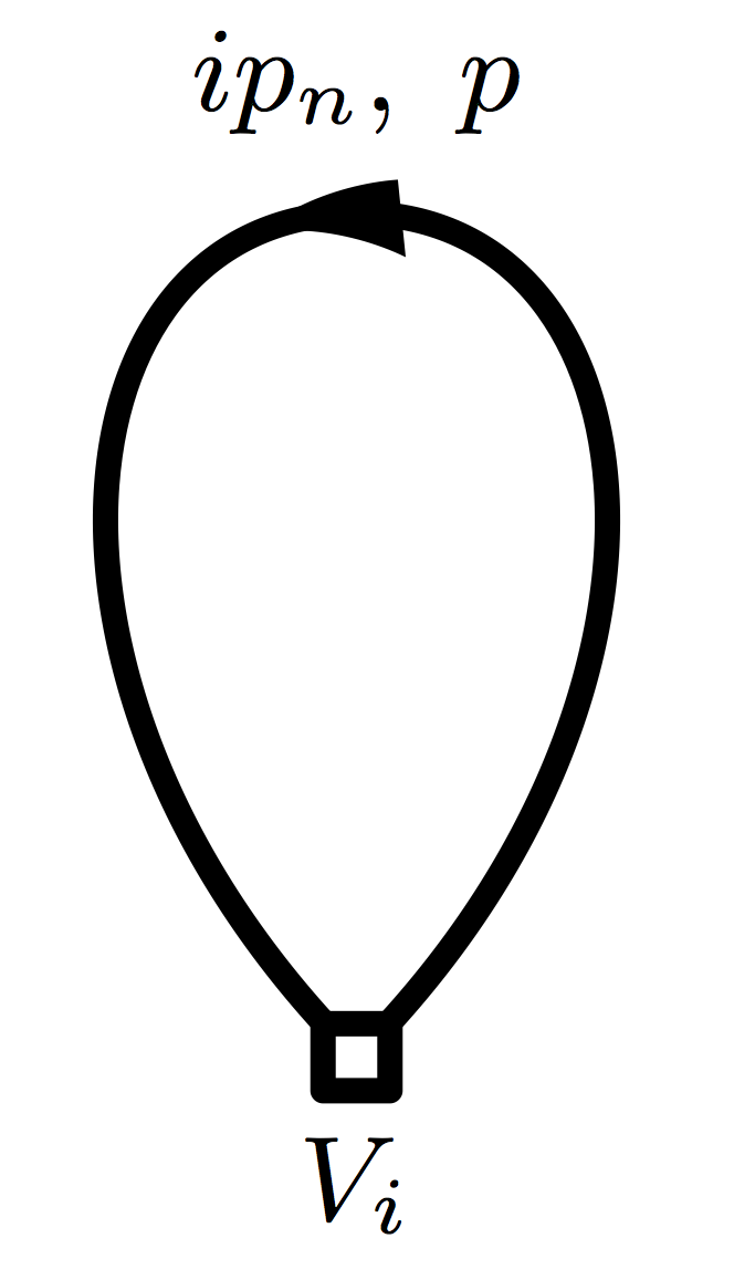
Figure 1: The general form of the self-energy diagram at first order. The first-order correction to the propagators $g^{11}(i\omega_{n},k)$ and $g^{22}(i\omega_{n},k)$ has $V_{i}=V_{2}$, whilst the anomalous propagators $g^{12}(i\omega_{n},k)$ and $g^{21}(i\omega_{n},k)$ have $V_{i}=V_{1}$ and $V_{i}=V_{1}^{*}$ respectively.

At first order, the diagrams that contribute to the self-energy are all of the form presented in Fig. 1. We begin by considering the diagonal matrix elements: the vertex in the self energy diagram is then given by $V_{i}=V_{2}$. The diagram corresponds to

$$({\bf\Sigma}(k))_{11} = -\sum_{ip_{n},p}\frac{4J}{\beta L}V_{2}(k,p,-k,-p)G_{0}(ip_{n},p)e^{ip_{n}0^{+}},$$ (20)

$$= \sum_{p}4JV_{2}(k,p,-p,-k)\frac{n_{F}(E_{p})}{L},$$

where $n_{F}(E_{p})=1/(\exp(\beta E_{p})+1)$ is the Fermi-Dirac distribution. The remaining momentum sum in Eq. (20) can only be performed numerically, as both the dispersion relation $E_{p}$ and the vertex function $V_{2}$ depend upon the Bogoliubov parameter $\theta_{k}$, which must be determined numerically from the self consistency condition (35).

We note that from the definition of the self-energy matrix and Eq. (20) it follows $({\bf\Sigma}(k))_{11}=-({\bf\Sigma}(k))_{22}$ as the same diagram contributes to both elements.

The off-diagonal elements of the self-energy matrix are given by the diagram in Fig. 1 with $V_{i}=V_{1}$ or $V_{i}=V_{1}^{*}=-V_{1}$. From this, it follows that $({\bf\Sigma}(k))_{12}=-({\bf\Sigma}(k))_{21}$ and the off-diagonal self-energy is given by

$$({\bf\Sigma}(k))_{12}=-6\sum_{p}JV_{1}(k,-k,p,-p)\frac{n_{F}(E_{p})}{L}.$$ (21)

From Eqs. (20)–(21) we see that the self-energy is frequency independent at first order in perturbation theory, hence Eq. (19) applies for calculating the modified single particle dispersion. The elements of the self-energy matrix are proportional to $J\lambda_{i}n_{F}(E_{p})$; the strongest corrections to the dispersion occur close to the minima of the dispersion (e.g. in the vicinity of the single particle gap) or when the system is at high temperatures. The single-particle dispersion with first order self-energy corrections is given by

$$\varepsilon_{k} = \pm\sqrt{\Big{(}E_{k}+4J\sum_{p}V_{2}(k,p,-p,-k)\frac{n_{F}(E_{p})}{L}\Big{)}^{2}+\left|6J\sum_{p}V_{1}(k,-k,p,-p)\frac{n_{F}(E_{p})}{L}\right|^{2}}\ .$$ (22)

At higher orders in perturbation theory the self-energy matrix becomes frequency dependent. This introduces additional poles in the Green’s function, corresponding to multi-particle excitations, which can be determined numerically.

IV Dynamical Structure Factor

The dynamical structure factor (DSF) $S(\omega,{\bf Q})$ is a frequency ($\omega$) and momentum (${\bf Q}$) resolved probe of the properties of a magnetic system

$$S^{\alpha\beta}(\omega,{\bf Q})=\frac{1}{L}\int_{-\infty}^{\infty}{\rm d}t\sum_{\ell,\ell^{\prime}}e^{i{\bf Q}\cdot(\bf{r}_{\ell}-\bf{r}_{\ell^{\prime}})}e^{i\omega t}\langle S^{\alpha}_{\ell}(t)S^{\beta}_{\ell^{\prime}}\rangle,$$

(23)

where $S^{\alpha}_{\ell}(t)=\exp(iHt)S^{\alpha}_{\ell}\exp(-iHt)$ is the time-evolved $\alpha$-component of the spin operator on site ${\bf r}_{\ell}$ of the lattice and $\langle{\cal O}\rangle$ denotes the thermal trace (9). The intensity measured in inelastic neutron scattering experiments is directly proportional to the DSFZaliznyak and Tranquada (2013a, b).

The calculation of the DSF for the Hamiltonian (1) is a very difficult problem. Fortunately we don’t require the full solution for our purposes. The key simplification arises from the fact that both $S^{zz}$ and $S^{yy}$ are dominated by features due to coherent single-particle modes, and in fact give the largest contribution to the measured DSF. These features can be described by a single-mode approximation, which gives a DSF of the form

$$S^{\alpha\alpha}(\omega,Q)\Bigg{|}_{\rm SMA} = A^{\alpha}(Q)\ \delta(\omega-\epsilon(Q))\ ,\ \alpha=y,z.$$ (24)

In the case of the transverse-field Ising chain, the exact one-particle contributions are knownHamer et al. (2006)

$$A^{y}(Q) = \left[1-\left(\frac{J}{h_{x}}\right)^{2}\right]^{1/4}\epsilon(Q)\ ,$$

$$A^{z}(Q) = \left[1-\left(\frac{J}{h_{x}}\right)^{2}\right]^{1/4}\frac{1}{\epsilon(Q)},$$

$$\epsilon(Q) = \sqrt{h_{x}^{2}-h_{x}J\cos(Q)+\frac{J^{2}}{4}}\ .$$ (25)

We will use that the inelastic neutron scattering data for ${\rm CoNb}_{2}{\rm O}_{6}$ in the paramagnetic phase exhibits a sharp response along the single particle dispersion in the $(\omega,Q)$-plane. This allows us (within experimental resolution) to extract the true single particle dispersion for excitations in ${\rm CoNb}_{2}{\rm O}_{6}$. We then fit the results of our perturbative calculation (22) to the extracted dispersion at a number of transverse field strengths to consistently fix the exchange parameters of our model (1).

IV.1 Fitting the single particle dispersion to experiment

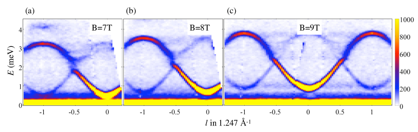
Figure 2: (Color online) Inelastic neutron scattering data probing the dispersion along the chain direction $l$ at (a) $B=7$ T; (b) $B=8$ T; (c) $B=9$ T. From this data the single particle dispersion (“Data” in Fig. 3) was extracted. Note the “anomalous broadening region” near $l\approx-0.55$ where the single-particle mode loses weight and significantly broadens. The incident neutron energy was $E_{i}=10$ meV.

In Fig. 2 we present inelastic neutron scattering data for the excitations along the chains for an applied transverse field of $B=7,8$ and $9$ T. The momentum along the chain direction is given in reciprocal lattice units of the crystallographic unit cell along the $c$-direction, i.e. $Q=l2\pi/c$ where $2\pi/c=1.247$Å^-1. As anticipated in the previous subsection, the data shows a single sharp quasi-particle excitation throughout the Brillouin zone (except in the vicinity of $l\sim-0.55$, which will be discussed later), with additional weak features due to multi-particle continua. The INS data at those three fields was parameterized using a 3D dispersion model (which takes into account also the weak interchain dispersion normal to the chains as explained in Ref. Cabrera et al., 2014), we then extract from this full parameterization the one-dimensional dispersion along the chain direction.

We then use a simulated annealing algorithmPress et al. (2005) to fit the results of our finite-temperature ($T\approx 50$ mK) perturbative calculation (22) to the observed one-dimensional single particle dispersion for three different values of the applied magnetic field. We run the simulated annealing algorithm in the $\{\lambda_{1},\lambda_{2},\lambda_{3}\}$ parameter space, varying the values of $J$ and $g_{x}\mu_{B}$ between runs and choose a set of parameters which consistently describes the single particle dispersion across the range of transverse field strengths. The best fit is obtained for the following set of parameters:

$$\begin{aligned} &J=-2.88~{}{\rm meV},\quad g_{x}=3.21,\\ &\lambda_{1}=-0.135,\quad\lambda_{2}=0.205,\quad\lambda_{3}=-0.003\ .\end{aligned}$$ (26)

Comparisons between the calculated single particle dispersion (solid line), exact diagonalization results for the Hamiltonian (1) with the above parameters and the extracted parameterization of the dispersion from inelastic neutron scattering data (Fig. 2) (dotted line) are shown in Figs. 3(a)-(c). We see that the perturbative calculation overestimates the single particle dispersion at $l\approx 1$ for $B=7$ T, but the exact diagonalization results are in excellent agreement with the experimental data for all fields. The perturbative calculation allows us to estimate the critical transverse field: the parameter set (26) leads to a one-dimensional critical field strength of $h_{C}=0.915$ meV ($B^{1D}_{C}\sim 4.92$ T), i.e. the field where the one-dimensional chains would have been critical in the absence of inter-chain couplings. We stress that our perturbative calculation is not controlled in the vicinity of the critical point, but this value broadly agrees with the experimental estimate of the 1D critical fieldColdea et al. (2010). The perturbative result for the critical field is also in excellent agreement with the field $h_{C}=0.908$ meV at which the extrapolated ($L=\infty$) single-particle gap vanishes in exact diagonalization studies of the Hamiltonian (1) with parameters (26).

(a) $B=7$T

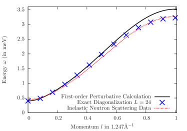
(b) $B=8$T

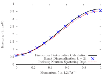
(c) $B=9$T

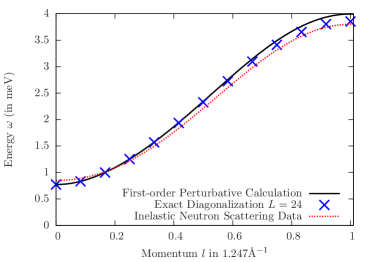
Figure 3: (Color online) Comparison between the single particle dispersion calculated by the perturbative calculation at $T\approx 50$ mK (solid line), exact diagonalization of the $L=24$ site system at $T=0$ (blue crosses) and the single particle dispersion extracted from the inelastic neutron scattering data of Fig. 2 (dotted line). We see that the perturbative calculation over estimates the single particle dispersion at $l\approx 1$ (especially for $B=7$ T), nevertheless exact diagonalization results match the experimental data very well.

In the following, we will use the parameter set (26) to carry out exact diagonalization studies of the DSF. Comparing these results to the INS data will lend further support to our claim that the model (1), (26) gives a good description of the one-dimensional physics of ${\rm CoNb}_{2}{\rm O}_{6}$.

IV.2 Exact diagonalization: Eigenvalue Spectrum

(a) $B=7$T

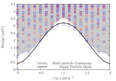
(b) $B=8$T

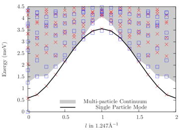
(c) $B=9$T

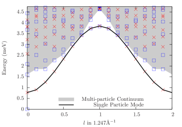
Figure 4: (Color online) We present the spectrum of the Hamiltonian (1) with parameters (26) obtained by exact diagonalization of the $L=16$ chain at (a) $B=7$ T; (b) $B=8$ T and (c) $B=9$ T. The parity under spin inversion $S^{z}\to-S^{z}$ of each state is labelled by crosses (odd) and squares (even). In particular we highlight the single particle mode (SPM) (solid line) and the multi-particle continuum (shaded region), showing that the SPM is close to or overlapping with the continuum for $l\approx 0.5-0.6$ in all three cases. There is a two-particle bound mode (blue squares below the continuum boundary) near the ferromagnetic zone boundary ($l=1$) with a similar energy to the SPM.

We start by considering the spectrum of the spin model (1), obtained by fully diagonalizing the Hamiltonian. This will be useful for our discussions of the DSF, particularly in describing the unusual broadening region (see Sec. V). Figures 4(a)–(c) present the spectrum of the Hamiltonian for $B=7,8,9$ T, where we have specified the symmetry of each state under spin inversion $S^{z}_{i}\to-S^{z}_{i}$. The single particle mode is shown as a solid line, while the extent of the multi-particle continua is indicated by the grey shaded region. In all three cases we see that the single particle mode grazes the two-particle continuum in the region $l=0.5-0.7$, with the three-particle continuum also close by at lower fields (within $\sim 0.25$ meV at $B=7$ T). This overlapping of the single particle mode with the multi-particle continuum is a result of physics beyond the transverse field Ising chain, for which this cannot occur in the paramagnetic phase due to kinematic constraints enforcing $E_{k}+E_{q-k}>E_{k}$ for all $k,q$.

IV.3 Lanczos diagonalization: The DSF

Having examined the spectrum of the Hamiltonian, we next turn our attention to the DSF. To study the DSF, we move away from full diagonalization of the Hamiltonian and use Lanczos based techniques to iteratively diagonalize the Hamiltonian, allowing us to work on much larger system sizes (up to $L=28$, where each momentum block of the Hamiltonian has dimension $\approx 2^{28}/28=9.6\times 10^{6}$). This significantly increases our momentum and frequency resolution, which will be useful in particular for examining the anomalous broadening region. We use that the diagonal components of the structure factor (23) can be written as

$$S^{\alpha\alpha}(\omega,Q)=\frac{1}{\pi}\lim_{\eta\to 0}\ {\rm Im}\ \langle S^{\alpha}_{Q}|\frac{1}{\omega+i\eta+E_{0}-H}|S^{\alpha}_{Q}\rangle,$$

where $S^{\alpha}_{Q}$ is the Fourier transform of the spin operator $S^{\alpha}_{l}$, $|S^{\alpha}_{Q}\rangle$ is the ground state with the Fourier transformed spin operator applied to it and $E_{0}$ is the ground state energy. In our numerics we take $\eta=0.01J$, which broadens the delta-functions peaks of the DSF by a Lorentzian.

Our procedure for calculating the diagonal components ($\alpha=x,y,z$) of the DSF is as follows: (i) we begin by using a Lanczos procedure to find the ground state; (ii) we construct the state obtained by acting on the ground state with the Fourier transformed spin operator; (iii) we perform an additional Lanczos procedure with the constructed state as the initial state and then calculate the DSF using the continued fraction representationGagliano and Balseiro (1987); Dagotto (1994).

(a)

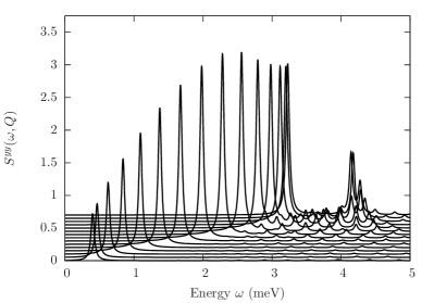
(b)

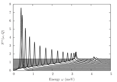
Figure 5: Constant wave vector cuts ($l=0\to 1$ in steps of $\delta l=1/14$, vertically displaced for clarity) of the dynamic structure factor $S^{\alpha\alpha}(\omega,Q=l2\pi/c)$ for (a) $\alpha=y$ and (b) $\alpha=z$ at $B=7$ T on the $L=28$ chain with Hamiltonian (1) and exchange parameter (26). We have used $120$ Lanczos iterations in the continued fraction and broadening parameter $\eta=0.01J$.

Following this procedure we find the DSF of the Hamiltonian (1) with exchange parameters (26) for $B=7,8,9$ T. We present the data for $B=7$ T in Fig. 5, where we have focussed on the $\alpha=y,z$ components of the DSF as these carry most of the spectral weight. The DSF is dominated by a single sharp mode across the Brillouin zone, with the multi-particle continua having non-negligible weight at $l\approx 1$ and $E\approx 4$ meV. This should be compared to the INS data presented in Fig. 2, where a similar feature is observed. As seen in experiment, with increasing applied transverse field $B$ the multi-particle feature moves to higher energies and becomes less intense. The single particle mode also moves up in energy with applied transverse field, as depicted in Figs. 3.

We see that whilst both the general features and the quantitative behaviour with transverse field of the DSF are captured by the minimal one-dimensional spin model (1), we do not see the anomalous broadening region observed in experimentsCabrera et al. (2014), see Fig. 2. In the next section we present high-resolution INS data for this phenomenon and propose a likely explanation of its origin.

V Anomalous broadening and quasi-particle breakdown

V.1 High resolution inelastic neutron scattering: Broadening region

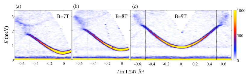
Figure 6: (Color online) High-resolution inelastic neutron scattering data for the single particle dispersion with momentum oriented along the chain. Note that the “anomalous broadening” region where the sharp mode loses weight and disappears is located distinctly away from the crystallographic zone boundary positions $l=\pm 0.5$ emphasized by vertical dotted lines. The data was obtained for neutrons with an incident energy of $E_{i}=4$ meV and a corresponding resolution on the elastic line of $\Delta E=0.051(1)$ meV. Data is shown for three applied transverse field strengths: (a) $B=7$ T; (b) $B=8$ T and (c) $B=9$ T.

A surprising feature of the INS data shown in Fig. 2, is that close to $l\approx 0.5$ the single particle mode appears to broaden and lose a significant amount of weight. Figure 6 presents high-resolution INS data (with resolution on the elastic line of $\Delta E=0.051(1)$ meV (FWHM)) focussed on this particular feature. The broadening and reduction in weight is so extreme, that at $B=7$ T a gap appears to have opened in the single particle mode; a careful analysis of the data shows that this feature does not occur at $l=-0.5$ but at wavevectors distinctly away from it (most clearly seen in Fig. 6, the “anomalous broadening” occurs away from the crystallographic zone boundary points $l=\pm 0.5$ indicated by vertical dotted lines). Hence it cannot be attributed to a zone boundary gap due to a doubling of the unit cell, such as seen in dimerization transitions (e.g. a Peierls transitionPeierls (1991)).

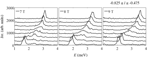
Figure 7: Scans through the neutron scattering data in Fig. 2 highlighting the anomalous broadening of the single particle mode in the region near $l\approx-0.55$. Traces (offset vertically and excluding error bars for clarity) correspond to the intensity as a function of energy in scans at fixed momentum l in the range $l=-0.475$ (lowest trace) to $l=-0.825$ (highest trace) in steps of 0.05 (each with an integration range of $\delta l=\pm 0.025$ around the nominal $l$-value) at (left) $B=7$ T, (center) $B=8$ T, and (right) $B=9$ T. Note the broadening of the peaks for energies $E(7~{}{\rm T})\approx 2.0-2.75$ meV, $E(8~{}{\rm T})\approx 2.25-3.0$ meV, and $E(9~{}{\rm T})\approx 2.5-3.25$ meV.

The change in the magnetic scattering intensity as a function of energy and momentum is shown in a series of constant-momentum cuts in Fig. 7, where we focus on the region of broadening $-0.825<l<-0.475$. The largest broadening and reduction of weight occurs when $B=7$ T in the energy range $E(7~{}{\rm T})\approx 2.0-2.75$ meV. At higher magnetic fields these features become less pronounced but are still clearly visible, with broadening observed for energies $E(8~{}{\rm T})\approx 2.25-3.0$ meV, and $E(9~{}{\rm T})\approx 2.5-3.25$ meV.

V.2 Broadening of the single particle mode at intermediate energies

In the remainder of this paper, we focus on explaining the “anomalous broadening” region in the INS data. The spin model introduced in Sec. III and the fit parameters of Sec. IV.1 serve as a starting point for exact diagonalization studies. As we have seen in the previous section, the DSF for the Hamiltonian (1) is dominated by a single dispersive mode that is sharp across the whole Brillouin zone and so does not capture the physics of the broadening of the single particle mode see in experiments. To go beyond this, we take inspiration from the data presented in Figs. 4(a)–(c), which show that the single particle mode and the multi-particle continuum overlap in the same region as the anomalous broadening is observed in the INS data. We also observe that the multi-particle excitations which are in the vicinity of the single particle mode are even under spin inversion symmetry, whilst the single particle mode is itself odd. As a result, transitions between the single particle mode and close by multi-particle excitations are forbidden in the Hamiltonian (1). Importantly, Figs. 4(a)–(c) also show that the multi-particle excitations in the vicinity of the single particle dispersion are even under spin inversion $S^{z}\to-S^{z}$, whilst the single particle mode is odd and so mixing of the two types of excitation is disallowed by the $\mathbb{Z}_{2}$ symmetry of the Hamiltonian. With this in mind, we add an additional term to the Hamiltonian (1) which breaks the $\mathbb{Z}_{2}$ spin inversion symmetry $S^{z}_{i}\to-S^{z}_{i}$ of the model: A natural candidate for such a term is a small longitudinal field $h_{z}=g_{z}\mu_{B}B_{z}$ which would arise in the experimental setting due to not having perfect alignment of the crystal with respect to the transverse field. Thus we consider the Hamiltonian modified by

$$H\to H+h_{z}\sum_{l}S^{z}_{l}\ .$$ (27)

For the inelastic neutron scattering data presented in Figs. 2, 6 and 7, it is estimated that the crystal was aligned such that the magnetic field was perpendicular to the Ising axis to within an accuracy of $\sim 1^{\circ}$.

It is worth noting that transitions between the 1 and 3 particle states can occur without the breaking of $S^{z}$ spin inversion symmetry. However, as can be seen in Figs 4(a)–(c), the three particle states are kinematically well separated from the single particle mode (no overlap), and decay $1\rightarrow 3$ can therefore not account for the anomalous broadening.

We also wish to highlight the fact that the overlap of the one-particle mode with the multi-particle continua does not occur within the paramagnetic phase of the transverse field Ising chain ($\lambda_{1}=\lambda_{2}=\lambda_{3}=0$): The overlap occurs in the present case due to the additional exchange interactions present in the Hamiltonian (1) which modify the dispersion shape such that an overlap of one and two-particle states exists for a finite field range above the critical field.

Let us now briefly summarize the requirements for the broadening of the single particle mode:

1. The single particle mode and the multi-particle continuum must overlap (see Figs. 4(a)–(c)).

2. Matrix elements must exist between the single particle mode and the overlapping states within the multi-particle continua. If these states are two-particle states, the $S^{z}$ spin inversion symmetry must be broken to allow transitions.

3. The decay rate of the single particle mode must be sufficiently large for the broadening to become apparent.

V.3 Lanczos Diagonalization (up to $L=28$)

We now turn to exact diagonalization results for the DSF in the presence of a small longitudinal field. As the broadening effect that we are looking for is seen in a certain area of the Brillouin zone, we use Lanczos diagonalization (and associated continued fraction techniquesGagliano and Balseiro (1987); Dagotto (1994)) to extend the momentum resolution of our calculations (for full diagonalization we are limited to $L\sim 18$ sites). We focus on the diagonal components of the DSF $S^{\alpha\alpha}(\omega,Q)$ with $\alpha=y,z$ as these carry most of the intensity. To allow us to compare the regions of anomalous broadening for different strength of the transverse field, we work with a fixed “crystal misalignment” of $\theta\sim 1.5^{\circ}$, and we use $g_{z}=5.9$ (we estimate from Ref. Kunimoto et al., 1999 that $g_{z}\approx 5.6-6.2$).

Fig. 8 shows the Lanczos results for the $\alpha=y,z$ components of the DSF in the $L=28$ chain at $B=7$ T with a misalignment of $\theta\sim 1.5^{\circ}$ ($h_{z}=0.062$meV). We see that when the single particle mode brushes the continuum (at $\omega\approx 2-2.5$ meV, cf. Fig. 4) the mode loses intensity and significantly broadens. This is consistent with the range of momenta $l\approx 0.5-0.7$ and frequency observed experimentally, see Figs. 2(a), 6(a) and 7(a). We see that the multi-particle continuum feature at $E\approx 4$ meV, $l\approx 1$ persists, which is also consistent with experiment.

(a)	(b)

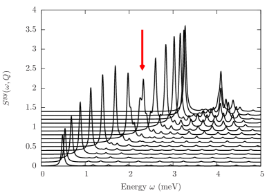
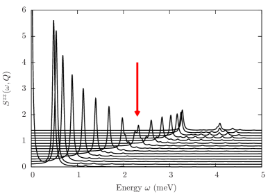
Figure 8: (Color online) Constant wave vector cuts ($l=0\to 1$ in steps of $\delta l=1/14$, vertically displaced for clarity) of the dynamic structure factor $S^{\alpha\alpha}(\omega,Q=l2\pi/c)$ for (a) $\alpha=y$ and (b) $\alpha=z$ for the $L=28$ site Hamiltonian (27) with transverse field $B=7$ T and misalignment of $\theta\sim 1.5^{\circ}$ ($h_{z}=0.062$ meV). We have used 120 Lanczos iterations in the continued fraction and broadening parameter $\eta=0.01J$. The arrow highlights the region of “anomalous broadening” of the single particle mode at $\omega\approx 2-2.5$ meV. The corresponding results for $h_{z}=0$ are shown in Fig. 5.

Analogous results for a field of $B=8$ T are shown Fig. 9. Compared to the $B=7$T data the region of anomalous broadening has shifted slightly in energy and momentum ($l\approx 0.55-0.75$) and the intensity loss is less pronounced, reflecting the decreased overlap between the single particle mode and the two-particle continuum, cf Fig. 4. Note that the shift in energy and momentum and decreased loss of intensity is also observed in the data, see Figs. 6(b) and 7(b).

(a)	(b)

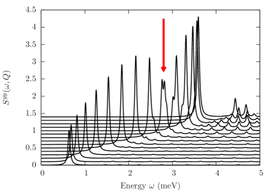
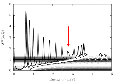
Figure 9: (Color online) Constant wave vector cuts ($l=0\to 1$ in steps of $\delta l=1/14$, vertically displaced for clarity) of the dynamic structure factor $S^{\alpha\alpha}(\omega,Q=l2\pi/c)$ for (a) $\alpha=y$ and (b) $\alpha=z$ for the $L=28$ site Hamiltonian (27) with transverse field $B=8$ T and misalignment of $\theta\sim 1.5^{\circ}$ ($h_{z}=0.072$ meV). We have used 120 Lanczos iterations in the continued fraction and broadening parameter $\eta=0.01J$. The arrow highlights the region of “anomalous broadening” of the single particle mode at $\omega\approx 2.5-3.5$ meV.

The numerical calculations predict that upon increasing the field further to $B=9$T the anomalous broadening region shifts to wavevectors near $l\sim 0.7$ and the broadening effect diminishes when compared to lower fields, compare Figs. 9 and Figs. 10. The experimental data in Figs. 6(a)–(c) indeed shows a shift with increasing field of the anomalous broadening region to higher energies along the dispersion bandwidth and to wavevectors further away from the $l=0.5$ zone boundary. However, the experimental data also shows that the anomalous region at $B=9$T extends over a wider energy range and the broadening effect is more pronounced in the experimental data (Fig. 6(c)) compared to the predictions of the theoretical model (Fig. 10). There could be a number of possible reasons for these differences in detail.

Firstly, the misalignment angle could be dependent on the applied field. This may be a result of the crystal not being completely rigid at high applied transverse fields. Whilst we have not extensively studied how the region of anomalous broadening moves with field-dependent misalignment, we have observed that increasing the longitudinal field at fixed transverse field results in the anomalous broadening becoming more severe and apparent over an increased range of momenta. Secondly, there could be terms in the Hamiltonian beyond those taken into account in our minimal model (1). This can lead to the movement of the multi-particle continua in phase space, and as a result a change in the region and severity of the anomalous broadening. Thirdly, the small system size $L=28$ in our exact diagonalization study may simply preclude an accurate description of the effect due to insufficient resolution in phase space or finite-size effects.

(a)	(b)

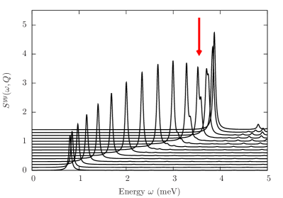
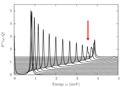
Figure 10: (Color online) Constant wave vector cuts ($l=0\to 1$ in steps of $\delta l=1/14$, vertically displaced for clarity) of the dynamic structure factor $S^{\alpha\alpha}(\omega,Q=l2\pi/c)$ for (a) $\alpha=y$ and (b) $\alpha=z$ for the $L=28$ site Hamiltonian (27) with transverse field $B=9$ T and misalignment of $\theta\sim 1.5^{\circ}$ ($h_{z}=0.081$ meV). We have used 120 Lanczos iterations in the continued fraction and broadening parameter $\eta=0.01J$. The arrow highlights the broadening region at $\omega\approx 3.5$ meV.

V.4 Quasi-particle breakdown

Above we have shown that the addition of a small longitudinal magnetic field component, consistent with small misalignment of the crystal in experiment, leads to the broadening of the single particle mode in the region $l\approx 0.5-0.7$ and that this broadening decreases with increased applied transverse field (for fixed misalignment). High resolution inelastic neutron scattering data in Figs. 6 and 7 show that this indeed occurs in experiment, with the single particle mode becoming extremely broad and carrying little spectral weight around $l=0.5-0.65$. The level of broadening observed in experiment is sufficient to say that the quasi-particles are no longer well defined over this region of the Brillouin zone, a phenomena known as “quasi-particle breakdown”Zhitomirsky and Chernyshev (2013).

A number of mechanisms for quasi-particle breakdown (and specifically “spontaneous magnon decay” in quantum magnets) are discussed in Refs. Zhitomirsky and Chernyshev, 2013; Fischer, 2011; Zhitomirsky, 2006; Kolezhuk and Sachdev, 2006; Bibikov, 2007; Fischer et al., 2010, 2011, including the case of field-induced decay. Most experimental observations of quasi-particle breakdown have so far been limited to the case where the single particle mode enters the two-particle continuum and terminates, such as in quasi-2D quantum magnetsStone et al. (2007) and quasi-1D spin-1 chainsMasuda et al. (2006).

In this case we observe something more unusual: two region of the Brillouin zone (0$\leq|l|\lesssim 0.5$ and $0.7\lesssim|l|\leq 1$) have coherent well-defined single particle excitations, whilst in the intermediate region $0.5\lesssim|l|\lesssim 0.7$ quasi-particle breakdown occurs. For the smallest fields that we examine ($B=7$ T) this effect is particularly severe in experiments (see Figs. 6(a) and 7(a)), where one could easily believe that a gap has opened in the single particle dispersion. Compare this to a similar field-tuned effect seen in the quasi-2D quantum magnet Ba₂MnGe₂O₇, where the excitation is broadened, but without the severe loss of intensity Masuda et al. (2010).

The quasi-particle breakdown in ${\rm CoNb}_{2}{\rm O}_{6}$ is a direct result of explicit symmetry breaking within the experimental setting, and highlights the crucial role that symmetry breaking perturbations can play.

VI Conclusions

Motivated by recent inelastic neutron scattering experimentsCabrera et al. (2014), we have investigated the origin of the anomalous broadening of the single particle dispersion in the quasi-one-dimensional ferromagnet ${\rm CoNb}_{2}{\rm O}_{6}$. We have presented high-resolution inelastic neutron scattering data (see Fig. 6) showing that the observed anomalous broadening has a non-trivial field dependence and is particularly severe at the small transverse field strengths (7 T), where the broadening may easily be mistaken for a gap in the single particle dispersion. To understand this behaviour, we have proposed a one-dimensional spin Hamiltonian whose parameters we fix by fitting the single particle dispersion to inelastic neutron scattering data presented in Fig. 2.

Having fixed the exchange parameters of our effective model, we add a single free parameter to our model – a longitudinal magnetic field. Such an addition is entirely reasonable, as we expect a small longitudinal field to arise from slight misalignment of the crystal in experiment. Crucially, this longitudinal field breaks spin inversion symmetry ($S^{z}\to-S^{z}$) which forbids transitions between the one-particle mode and the two-particle continuum. The breaking of this symmetry has a profound effect on the dynamical structure factor of the quantum spin model – in regions of the Brillouin zone where the two-particle continuum overlaps with the single particle mode (see Fig. 4) we see that the single particle mode loses weight and broadens (see Figs. 8 and 9 for exact diagonalization data). This broadening occurs due to the longitudinal field inducing the spontaneous decay of the single particle excitation into multi-particle excitations, an example of “quasi-particle breakdown”Zhitomirsky and Chernyshev (2013). ${\rm CoNb}_{2}{\rm O}_{6}$ is particularly unusual in this regard as the region of quasi-particle breakdown separates two regions of coherent quasi-particles in the Brillouin zone.

Acknowledgements. This work was supported by the EPSRC under Grants No. EP/I032487/1 (FHLE and NJR) and EP/H014934/1 (RC and IC).

Appendix A Transforming the spin Hamiltonian (1) into the fermion Hamiltonian (2)

Starting from the Hamiltonian (1), we start by rotating the spin quantization axes by $\pi/2$ about $S^{y}$ to be in keeping with standard conventions. We then perform a Jordan-Wigner transformation and subsequently Fourier transform the resulting fermionic theory to obtain the momentum space Hamiltonian $H=H_{0}+H_{{\rm int}}+E_{0}$ where $E_{0}$ is an additive constant that rescales the absolute energy and is neglected herein, $H_{0}$ contains only fermion bilinears and $H_{\rm int}$ is quartic in the fermion operators

$$H_{0} = \frac{1}{2}\sum_{k}\Big{(}c^{\dagger}_{k}~{}~{}c_{-k}\Big{)}\left(\begin{array}[]{cc}A_{k}&iB_{k}\\ -iB_{k}&-A_{k}\end{array}\right)\left(\begin{array}[]{c}c_{k}\\ c_{-k}^{\dagger}\end{array}\right),$$ (32)

$$H_{{\rm int}} = \frac{J}{2L}(\lambda_{1}-\lambda_{3})\sum_{k_{i}}\Big{[}f_{(k_{1},k_{2},k_{3})(k_{4})}c_{k_{1}}^{\dagger}c_{k_{2}}^{\dagger}c_{k_{3}}^{\dagger}c_{-k_{4}}+{\rm H.c.}\Big{]}$$

$$- \frac{J}{2L}\sum_{k_{i}}\Big{[}2\lambda_{2}h_{(k_{1},k_{2})(k_{3},k_{4})}+2\lambda_{3}h_{(2k_{1},2k_{2})(2k_{3},2k_{4})}+(\lambda_{1}+\lambda_{3})g_{(k_{1},k_{2})(k_{3},k_{4})}\Big{]}c^{\dagger}_{k_{1}}c^{\dagger}_{k_{2}}c_{-k_{3}}c_{-k_{4}},$$

The matrix elements of $H_{0}$ are given by

$$A_{k} = \frac{J}{2}(1+\lambda_{2})\cos(k)+\frac{J}{2}(\lambda_{1}+\lambda_{3})\cos(2k)+h_{x}-J(\lambda_{2}+\lambda_{3}),$$

$$B_{k} = -\frac{J}{2}(1-\lambda_{2})\sin(k)-\frac{J}{2}(\lambda_{1}-\lambda_{3})\sin(2k),$$

whilst the vertex factors appearing in $H_{\rm int}$ take the form

$$f_{(k_{1},k_{2},k_{3})(k_{4})} = \frac{i}{3}\left[\sin(k_{3}-k_{1})+\sin(k_{1}-k_{2})+\sin(k_{2}-k_{3})\right]\delta_{\sum_{j}k_{j},0},$$

$$g_{(k_{1},k_{2})(k_{3},k_{4})} = \frac{1}{2}\left[\cos(k_{4}-k_{1})-\cos(k_{4}-k_{2})+\cos(k_{3}-k_{2})-\cos(k_{3}-k_{1})\right]\delta_{\sum_{j}k_{j},0},$$

$$h_{(k_{1},k_{2})(k_{3},k_{4})} = \frac{1}{4}\left[\cos(k_{1}+k_{3})-\cos(k_{2}+k_{3})+\cos(k_{2}+k_{4})-\cos(k_{1}+k_{4})\right]\delta_{\sum_{j}k_{j},0},$$

which are antisymmetric under pair-wise exchange of indices appearing within the same brackets $(\ldots)$ and impose momentum conservation.

We now diagonalize the quadratic part of the Hamiltonian by performing a self-consistent Bogoliubov transformation. We define the Bogoliubov fermions $a_{k}$ by

$$c^{\dagger}_{k}=-i\cos\theta_{k}a^{\dagger}_{k}-\sin\theta_{k}a_{-k},\qquad c_{k}=i\cos\theta_{k}a_{k}-\sin\theta_{k}a^{\dagger}_{-k},$$ (33)

where the Bogoliubov parameter $\theta_{k}=-\theta_{-k}$ satisfies the self-consistency condition $A_{k}\sin(2\theta_{k})-B_{k}\cos(2\theta_{k})=0$. The quadratic part of the Hamiltonian then becomes diagonal

$$H_{0}=\frac{1}{2}\sum_{k}\Big{(}a^{\dagger}_{k}~{}~{}a_{-k}\Big{)}\left(\begin{array}[]{cc}\sqrt{A_{k}^{2}+B_{k}^{2}}&0\\ 0&-\sqrt{A_{k}^{2}+B_{k}^{2}}\end{array}\right)\left(\begin{array}[]{c}a_{k}\\ a_{-k}^{\dagger}\end{array}\right).$$ (34)

Let us now consider the action of the Bogoliubov transformation (33) on the interaction term of the Hamiltonian $H_{\rm int}$. It is clear that many of the transformed terms in $H_{\rm int}$ will not be normal ordered. The normal ordering of these terms will generate fermion bilinear terms that contribute to both the diagonal and off-diagonal elements of $H_{0}$ in Eq. (34). In order that the quadratic part of the Hamiltonian is diagonal, we impose a self-consistency condition on the Bogoliubov parameter: it must be chosen such that the off-diagonal terms that result from normal-ordering interaction terms vanish. The resulting self-consistency condition for the Bogoliubov parameter is

$$\bigg{[}A_{k}+\sum_{q}\Theta_{1}(k,q)\bigg{]}\sin 2\theta_{k}-\bigg{[}B_{k}+\sum_{q}\Theta_{2}(k,q)\bigg{]}\cos 2\theta_{k}=0,$$ (35)

where we have defined the functions

$$\Theta_{1}(k,q) = -\frac{4J}{L}\bigg{[}\frac{1}{2}(\lambda_{1}+\lambda_{3})g_{(k,q)(-q,-k)}+\lambda_{2}h_{(k,q)(-q,-k)}+\lambda_{3}h_{(2k,2q)(-2q,-2k)}\bigg{]}\sin^{2}\theta_{q}$$

$$+\frac{3J}{2L}(\lambda_{1}-\lambda_{3})if_{(k,q,-q)(-k)}\sin 2\theta_{q},$$

$$\Theta_{2}(k,q) = \frac{J}{L}\bigg{[}\frac{1}{2}(\lambda_{1}+\lambda_{3})g_{(k,-k)(q,-q)}+\lambda_{2}h_{(k,-k)(q,-q)}+\lambda_{3}h_{(2k,-2k)(2q,-2q)}\bigg{]}\sin 2\theta_{q}$$

$$+\frac{3J}{L}(\lambda_{1}-\lambda_{3})if_{(k,q,-k)(-q)}\sin^{2}\theta_{q},$$

which also depend upon the Bogoliubov parameter.

The self-consistency condition (35) perturbatively modifies the Bogoliubov parameter. Due to the complicated structure Eq. (35), we solve the set of non-linear simultaneous equations numerically using standard techniques. Following the imposition of the self-consistency condition, we obtain the Hamiltonian (2) with dispersion relation (LABEL:SelfConE).

Appendix B Vertex functions

The vertex functions $V_{0},~{}V_{1},~{}V_{2}$ in Eq. (2) are obtained by normal-ordering of the four-fermion terms after Bogoliubov transformation. By symmetry, they can be expressed in terms of summations over permutations of indices. For example

$$V_{0}(k_{1},k_{2},k_{3},k_{4}) = \delta_{\sum_{j}k_{j},0}\Bigg{\{}\frac{1}{96}\left(\lambda_{3}-\lambda_{1}\right)\sum_{P\in S_{4}}{\rm sgn}(P)\cos\bigg{[}k_{P_{1}}-k_{P_{2}}+\theta_{k_{P_{1}}}+\theta_{k_{P_{2}}}+\theta_{k_{P_{3}}}-\theta_{k_{P_{4}}}\bigg{]}$$

$$+\frac{1}{96}\sum_{j=2}^{3}\lambda_{j}\sum_{P\in S_{4}}{\rm sgn}(P)\cos\bigg{[}(j-1)\Big{(}k_{P_{1}}+k_{P_{2}}\Big{)}+\theta_{k_{P_{1}}}-\theta_{k_{P_{2}}}+\theta_{k_{P_{3}}}-\theta_{k_{P_{4}}}\bigg{]}\Bigg{\}}\ ,$$

where the permutation $P$ acts on the set $P:\{1,2,3,4\}\to\{P_{1},P_{2},P_{3},P_{4}\}$.

The vertex which changes quasi-particle number by two is given by

$$V_{1}(k_{1},k_{2},k_{3},k_{4})=\delta_{\sum_{j}k_{j},0}\bigg{[}V_{1}^{(12)}(k_{1},k_{2},k_{3},k_{4})+V_{1}^{(23)}(k_{1},k_{2},k_{3},k_{4})+V_{1}^{(13)}(k_{1},k_{2},k_{3},k_{4})\bigg{]},$$

where

$$V_{1}^{(12)}(k_{1},k_{2},k_{3},k_{4}) = \frac{i}{24}\left(\lambda_{1}-\lambda_{2}\right)\sum_{Q\in S_{3}}{\rm sgn}(Q)\Bigg{\{}\sin\bigg{[}k_{Q_{1}}-k_{4}+\theta_{k_{Q_{1}}}-\theta_{k_{Q_{2}}}+\theta_{k_{Q_{3}}}-\theta_{k_{4}}\bigg{]}$$

$$\hskip 108.12054pt+\sin\bigg{[}k_{Q_{1}}-k_{4}-\theta_{k_{Q_{1}}}+\theta_{k_{Q_{2}}}-\theta_{k_{Q_{3}}}+\theta_{k_{4}}\bigg{]}$$

$$\hskip 108.12054pt-\sin\bigg{[}k_{Q_{1}}-k_{Q_{2}}+\theta_{k_{Q_{1}}}-\theta_{k_{Q_{2}}}-\theta_{k_{Q_{3}}}+\theta_{k_{4}}\bigg{]}$$

$$\hskip 108.12054pt-\sin\bigg{[}k_{Q_{1}}-k_{Q_{2}}-\theta_{k_{Q_{1}}}+\theta_{k_{Q_{2}}}-\theta_{k_{Q_{3}}}+\theta_{k_{4}}\bigg{]}\Bigg{\}},$$

$$V_{1}^{(23)}(k_{1},k_{2},k_{3},k_{4}) = -\frac{i}{24}\sum_{j=2}^{3}\lambda_{j}\sum_{Q\in S_{3}}{\rm sgn}(Q)\Bigg{\{}\sin\bigg{[}(j-1)\Big{(}k_{Q_{1}}+k_{Q_{2}}\Big{)}-\theta_{k_{Q_{1}}}+\theta_{k_{Q_{2}}}-\theta_{k_{Q_{3}}}+\theta_{k_{4}}\bigg{]}$$

$$\hskip 102.43008pt+\sin\bigg{[}(j-1)\Big{(}k_{Q_{1}}+k_{Q_{2}}\Big{)}-\theta_{k_{Q_{1}}}+\theta_{k_{Q_{2}}}+\theta_{k_{Q_{3}}}-\theta_{k_{4}}\bigg{]}$$

$$\hskip 102.43008pt+\sin\bigg{[}(j-1)\Big{(}k_{Q_{1}}+k_{4}\Big{)}+\theta_{k_{Q_{1}}}-\theta_{k_{Q_{2}}}+\theta_{k_{Q_{3}}}-\theta_{k_{4}}\bigg{]}$$

$$\hskip 102.43008pt+\sin\bigg{[}(j-1)\Big{(}k_{Q_{1}}+k_{4}\Big{)}-\theta_{k_{Q_{1}}}-\theta_{k_{Q_{2}}}+\theta_{k_{Q_{3}}}+\theta_{k_{4}}\bigg{]}\Bigg{\}},$$

$$V_{1}^{(13)}(k_{1},k_{2},k_{3},k_{4}) = \frac{i}{24}(\lambda_{1}+\lambda_{3})\sum_{Q\in S_{3}}{\rm sgn}(Q)\Bigg{\{}\sin\bigg{[}k_{Q_{1}}-k_{Q_{2}}-\theta_{k_{Q_{1}}}+\theta_{k_{Q_{2}}}+\theta_{k_{Q_{3}}}-\theta_{k_{4}}\bigg{]}$$

$$\hskip 108.12054pt-\sin\bigg{[}k_{Q_{1}}-k_{Q_{2}}+\theta_{k_{Q_{1}}}-\theta_{k_{Q_{2}}}-\theta_{k_{Q_{3}}}+\theta_{k_{4}}\bigg{]}$$

$$\hskip 108.12054pt+\sin\bigg{[}k_{Q_{1}}-k_{4}+\theta_{k_{Q_{1}}}-\theta_{k_{Q_{2}}}+\theta_{k_{Q_{3}}}-\theta_{k_{4}}\bigg{]}$$

$$\hskip 108.12054pt-\sin\bigg{[}k_{Q_{1}}-k_{4}-\theta_{k_{Q_{1}}}+\theta_{k_{Q_{2}}}-\theta_{k_{Q_{3}}}+\theta_{k_{4}}\bigg{]}\Bigg{\}}.$$

Here in $V_{1}^{(12)}$, $V_{1}^{(23)}$ and $V_{1}^{(13)}$ the permutation $Q$ acts on the set $Q:\{1,2,3\}\to\{Q_{1},Q_{2},Q_{3}\}$.

The remaining vertex function that preserves quasiparticle number is given by

$$V_{2}(k_{1},k_{2},k_{3},k_{4})=\delta_{\sum_{j}k_{j},0}\bigg{[}V_{2}^{(1)}(k_{1},k_{2},k_{3},k_{4})+V_{2}^{(23)}(k_{1},k_{2},k_{3},k_{4})+V_{2}^{(3)}(k_{1},k_{2},k_{3},k_{4})\bigg{]},$$

with

$$V^{(1)}_{2}(k_{1},k_{2},k_{3},k_{4}) = \frac{\lambda_{1}}{4}\sum_{P,Q\in S_{2}}{\rm sgn}(P){\rm sgn}(Q)\Bigg{\{}\cos\bigg{[}k_{P_{1}}-k_{P_{2}}+\theta_{k_{1}}-\theta_{k_{2}}+\theta_{k_{Q_{3}}}-\theta_{k_{Q_{4}}}\bigg{]}$$

$$\hskip 105.2751pt+\cos\bigg{[}k_{Q_{3}}-k_{Q_{4}}+\theta_{k_{3}}-\theta_{k_{4}}+\theta_{k_{P_{1}}}-\theta_{k_{P_{2}}}\bigg{]}$$

$$\hskip 105.2751pt+\cos\bigg{[}k_{P_{1}}-k_{Q_{3}}+\theta_{k_{P_{1}}}+\theta_{k_{P_{2}}}-\theta_{k_{Q_{3}}}-\theta_{k_{Q_{4}}}\bigg{]}$$

$$\hskip 105.2751pt+\cos\bigg{[}k_{P_{1}}-k_{Q_{3}}+\theta_{k_{P_{1}}}-\theta_{k_{P_{2}}}-\theta_{k_{Q_{3}}}+\theta_{k_{Q_{4}}}\bigg{]}\Bigg{\}},$$

$$V^{(23)}(k_{1},k_{2},k_{3},k_{4}) = \frac{1}{8}\sum_{j=2}^{3}\lambda_{j}\sum_{P,Q\in S_{2}}{\rm sgn}(P){\rm sgn}(Q)\Bigg{\{}\cos\bigg{[}(j-1)\Big{(}k_{P_{1}}+k_{P_{2}}\Big{)}+\theta_{k_{1}}-\theta_{k_{2}}-\theta_{k_{Q_{3}}}+\theta_{k_{Q_{4}}}\bigg{]}$$

$$\hskip 128.0374pt+\cos\bigg{[}(j-1)\Big{(}k_{Q_{3}}+k_{Q_{4}}\Big{)}+\theta_{k_{3}}-\theta_{k_{4}}-\theta_{k_{P_{1}}}+\theta_{k_{P_{2}}}\bigg{]}$$

$$\hskip 128.0374pt-\cos\bigg{[}(j-1)\Big{(}k_{P_{1}}+k_{Q_{3}}\Big{)}+\theta_{k_{P_{1}}}+\theta_{k_{P_{2}}}-\theta_{k_{Q_{3}}}-\theta_{k_{Q_{4}}}\bigg{]}$$

$$\hskip 128.0374pt-\cos\bigg{[}(j-1)\Big{(}k_{P_{1}}+k_{Q_{3}}\Big{)}+\theta_{k_{P_{1}}}-\theta_{k_{P_{2}}}-\theta_{k_{Q_{3}}}+\theta_{k_{Q_{4}}}\bigg{]}$$

$$\hskip 128.0374pt-\cos\bigg{[}(j-1)\Big{(}k_{P_{1}}+k_{Q_{3}}\Big{)}-\theta_{k_{P_{1}}}-\theta_{k_{P_{2}}}+\theta_{k_{Q_{3}}}+\theta_{k_{Q_{4}}}\bigg{]}$$

$$\hskip 128.0374pt-\cos\bigg{[}(j-1)\Big{(}k_{P_{1}}+k_{Q_{3}}\Big{)}-\theta_{k_{P_{1}}}+\theta_{k_{P_{2}}}+\theta_{k_{Q_{3}}}-\theta_{k_{Q_{4}}}\bigg{]}\Bigg{\}},$$

$$V_{2}^{(3)}(k_{1},k_{2},k_{3},k_{4}) = \frac{\lambda_{3}}{4}\sum_{P,Q\in S_{2}}{\rm sgn}(P){\rm sgn}(Q)\Bigg{\{}\cos\bigg{[}k_{P_{1}}-k_{Q_{3}}-\theta_{k_{P_{1}}}+\theta_{k_{P_{2}}}+\theta_{k_{Q_{3}}}-\theta_{k_{Q_{4}}}\bigg{]}$$

$$\hskip 105.2751pt+\cos\bigg{[}k_{P_{1}}-k_{Q_{3}}-\theta_{k_{P_{1}}}-\theta_{k_{P_{2}}}+\theta_{k_{Q_{3}}}+\theta_{k_{Q_{4}}}\bigg{]}\Bigg{\}},$$

where $P$ is the permutation acting on the set $P:\{1,2\}\to\{P_{1},P_{2}\}$ and the permutation $Q$ acts on the set $Q:\{3,4\}\to\{Q_{3},Q_{4}\}$.

References

- Cabrera et al. (2014) I. Cabrera, J. D. Thompson, R. Coldea, D. Prabhakaran, R. I. Bewley, T. Guidi, J. A. Rodriguez-Rivera, and C. Stock, Phys. Rev. B 90, 014418 (2014).
- Anderson (1952) P. W. Anderson, Phys. Rev. 86, 694 (1952).
- Kubo (1952) R. Kubo, Phys. Rev. 87, 568 (1952).
- Kubo (1953) R. Kubo, Rev. Mod. Phys. 25, 344 (1953).
- Dyson (1956a) F. J. Dyson, Phys. Rev. 102, 1217 (1956a).
- Dyson (1956b) F. J. Dyson, Phys. Rev. 102, 1230 (1956b).
- Van Kranendonk and Van Vleck (1958) J. Van Kranendonk and J. H. Van Vleck, Rev. Mod. Phys. 30, 1 (1958).
- Akhiezer et al. (1958) A. I. Akhiezer, V. G. Bar’yakhtar, and S. V. Peletminskii, Spin Waves (North-Holland, 1958).
- Mattis (1981) D. C. Mattis, The Theory of Magnetism (Springer, 1981).
- Pauthenet (1982) R. Pauthenet, Journal of Applied Physics 53, 8187 (1982).
- Manousakis (1991) E. Manousakis, Rev. Mod. Phys. 63, 1 (1991).
- Zhitomirsky and Chernyshev (1999) M. E. Zhitomirsky and A. L. Chernyshev, Phys. Rev. Lett. 82, 4536 (1999).
- Hagiwara et al. (2005) M. Hagiwara, L. P. Regnault, A. Zheludev, A. Stunault, N. Metoki, T. Suzuki, S. Suga, K. Kakurai, Y. Koike, P. Vorderwisch, and J.-H. Chung, Phys. Rev. Lett. 94, 177202 (2005).
- Veillette et al. (2005) M. Y. Veillette, A. J. A. James, and F. H. L. Essler, Phys. Rev. B 72, 134429 (2005).
- Suzuki and Suga (2005) T. Suzuki and S.-i. Suga, Phys. Rev. B 72, 014434 (2005).
- Stone et al. (2007) M. B. Stone, I. A. Zaliznyak, T. Hong, C. L. Broholm, and D. H. Reich, Nature 440, 187 (2007).
- Zhitomirsky (2006) M. E. Zhitomirsky, Phys. Rev. B 73, 100404 (2006).
- Masuda et al. (2006) T. Masuda, A. Zheludev, H. Manaka, L.-P. Regnault, J.-H. Chung, and Y. Qiu, Phys. Rev. Lett. 96, 047210 (2006).
- Kolezhuk and Sachdev (2006) A. Kolezhuk and S. Sachdev, Phys. Rev. Lett. 96, 087203 (2006).
- Bibikov (2007) P. N. Bibikov, Phys. Rev. B 76, 174431 (2007).
- Syljuåsen (2008) O. F. Syljuåsen, Phys. Rev. B 78, 180413 (2008).
- Lüscher and Läuchli (2009) A. Lüscher and A. M. Läuchli, Phys. Rev. B 79, 195102 (2009).
- Chernyshev and Zhitomirsky (2009) A. L. Chernyshev and M. E. Zhitomirsky, Phys. Rev. B 79, 144416 (2009).
- Masuda et al. (2010) T. Masuda, S. Kitaoka, S. Takamizawa, N. Metoki, K. Kaneko, K. C. Rule, K. Kiefer, H. Manaka, and H. Nojiri, Phys. Rev. B 81, 100402 (2010).
- Fischer et al. (2010) T. Fischer, S. Duffe, and G. S. Uhrig, New J. of Phys. 12, 033048 (2010).
- Syromyatnikov (2010) A. V. Syromyatnikov, Phys. Rev. B 82, 024432 (2010).
- Stephanovich and Zhitomirsky (2011) V. A. Stephanovich and M. E. Zhitomirsky, EPL (Europhysics Letters) 95, 17007 (2011).
- Fischer et al. (2011) T. Fischer, S. Duffe, and G. S. Uhrig, EPL (Europhysics Letters) 96, 47001 (2011).
- Fischer (2011) T. Fischer, Description of quasiparticle decay by continuous unitary transformations, Ph.D. thesis, TU-Dortmund (2011).
- Doretto and Vojta (2012) R. L. Doretto and M. Vojta, Phys. Rev. B 85, 104416 (2012).
- Fuhrman et al. (2012) W. T. Fuhrman, M. Mourigal, M. E. Zhitomirsky, and A. L. Chernyshev, Phys. Rev. B 85, 184405 (2012).
- Zhitomirsky and Chernyshev (2013) M. E. Zhitomirsky and A. L. Chernyshev, Rev. Mod. Phys. 85, 219 (2013).
- Oh et al. (2013) J. Oh, M. D. Le, J. Jeong, J.-H. Lee, H. Woo, W.-Y. Song, T. G. Perring, W. J. L. Buyers, S.-W. Cheong, and J.-G. Park, Phys. Rev. Lett. 111, 257202 (2013).
- Mourigal et al. (2013) M. Mourigal, W. T. Fuhrman, A. L. Chernyshev, and M. E. Zhitomirsky, Phys. Rev. B 88, 094407 (2013).
- Pfeuty (1970) P. Pfeuty, Annals of Physics 57, 79 (1970).
- Chakrabati et al. (1996) B. K. Chakrabati, A. Dutta, and P. Sen, Quantum Ising Phases and Transitions in Transverse Ising Models (Springer, 1996).
- Sachdev (1999) S. Sachdev, Quantum Phase Transitions (Cambridge University Press, 1999).
- Coldea et al. (2010) R. Coldea, D. A. Tennant, E. M. Wheeler, E. Wawrzynska, D. Prabhakaran, M. Telling, K. Habicht, P. Smeibidl, and K. Kiefer, Science 327, 177 (2010).
- Zamolodchikov (1989) A. B. Zamolodchikov, Int. J. Mod. Phys. A 04, 4235 (1989).
- Morris et al. (2014) C. M. Morris, R. Valdés Aguilar, A. Ghosh, S. M. Koohpayeh, J. Krizan, R. J. Cava, O. Tchernyshyov, T. M. McQueen, and N. P. Armitage, Phys. Rev. Lett. 112, 137403 (2014).
- Kjäll et al. (2011) J. A. Kjäll, F. Pollmann, and J. E. Moore, Phys. Rev. B 83, 020407 (2011).
- Essler and Konik (2005) F. H. L. Essler and R. M. Konik, in From Fields to Strings: Circumnavigating Theoretical Physics, edited by A. Vainshtein and J. Wheater (World Scientific, Singapore, 2005) arXiv:cond-mat/0412421 .
- Hamer et al. (2006) C. J. Hamer, J. Oitmaa, Z. Weihong, and R. H. McKenzie, Phys. Rev. B 74, 060402 (2006).
- James et al. (2009) A. J. A. James, W. D. Goetze, and F. H. L. Essler, Phys. Rev. B 79, 214408 (2009).
- Zaliznyak and Tranquada (2013a) I. Zaliznyak and J. M. Tranquada, Neutron Scattering and Its Application to Strongly Correlated Systems, edited by A. Avella and F. Mancini (Springer, 2013).
- Zaliznyak and Tranquada (2013b) I. Zaliznyak and J. M. Tranquada, ArXiv e-prints (2013b), arXiv:1304.4214 .
- Press et al. (2005) W. H. Press, S. A. Teukolsky, W. T. Vetterling, and B. P. Flannery, Numerical Recipes in C++ (Cambridge University Press, 2005).
- Gagliano and Balseiro (1987) E. R. Gagliano and C. A. Balseiro, Phys. Rev. Lett. 59, 2999 (1987).
- Dagotto (1994) E. Dagotto, Rev. Mod. Phys. 66, 763 (1994).
- Peierls (1991) R. Peierls, More Surprises in Theoretical Physics (Princeton University Press, 1991).
- Note (1) One may think that off-diagonal elements of the -tensor might have the same effect. However, as a result of the local symmetry point group at the Co2+ site (two-fold rotation axis around ), the -axis is a principle axis of the -tensor so an external magnetic field applied strictly along the -axis does not induce a longitudinal field component.
- Kunimoto et al. (1999) T. Kunimoto, K. Nagasaka, H. Nojiri, S. Luther, M. Motokawa, H. Ohta, T. Goto, S. Okubo, and K. Kohn, Journal of the Physical Society of Japan 68, 1703 (1999).