Anomalous top charged-current contact interactions in single top production at the LHC

Abstract

In an effective theory approach, the full minimal set of leading contributions to anomalous charged-current top couplings comprises various new trilinear $tbW$ as well as quartic $tbf\!f^{\prime}$ interaction vertices, some of which are related to one another by equations of motion. While much effort in earlier work has gone into the extraction of the trilinear couplings from single top measurements, we argue in this article that these structures can be assessed independently by other observables, while single top production forms a unique window to the four-fermion sector. An effective theory approach is employed to infer and classify the minimal set of such couplings from dimension six operators in the minimal flavor violation scheme. In the phenomenological analysis, we present a Monte Carlo study at detector level to quantify the expected performance of the next LHC run to bound as well as distinguish the various contact couplings. Special attention is directed toward differential final state distributions including detector effects as a means to optimize the signal sensitivity as well as the discriminative power with respect to the possible coupling structures.

I Introduction

It was with considerable public attention that the two LHC experiments ATLAS Aad et al. (2008, 2009) and CMS Chatrchyan et al. (2008) finally claimed their discovery of a Higgs-like resonance in summer 2012 Aad et al. (2012a); Chatrchyan et al. (2012a), with subsequent investigations ever further backing up the picture that this new particle might indeed be the standard model (SM) Higgs in its simplest form Chatrchyan et al. (2013a); Aad et al. (2013a, b). However, this result, which at first glance appears as the ultimate triumph of the theory, might turn out as a mixed blessing because the more profound puzzle, namely the dynamical mechanism which triggers electroweak symmetry breaking (EWSB) and potentially stabilizes the Higgs mass beyond tree level, remains as obscure as ever in the absence of any new physics (NP) beyond the SM (BSM). From this point of view, even if no new degrees of freedom are in sight, NP could manifest itself in slight deviations of SM predictions in various parameters such as couplings or widths. Revealing these effects requires two ingredients, namely the identification and precise measurement of promising observables, but also a solid theoretical description in order to parametrize their dependence on NP scenarios in a consistent manner.

Apart from the Higgs particle itself the top sector represents a natural arena to assess the puzzle of EWSB, because of the large top mass of the order of the EWSB scale itself, which has two important consequences: First, the top has a robust $\mathcal{O}(1)$ Yukawa coupling to the symmetry breaking sector, making it a natural probe for its detailed layout. Second, it is hard to access experimentally, so that its properties have not been determined to very high precision until now by direct measurements. Even if top-Higgs couplings will remain poorly bounded for quite a while yet, also its electroweak interactions such as anomalous charged-current (CC) couplings $tbW$ and $tbf\!f^{\prime}$ may be driven by EWSB details. These couplings can already be constrained by direct measurements at the LHC via top decays as well as single top production. For example, top pair production (forming the basis for decay measurements) has been measured in various channels by the LHC multipurpose experiments ATLAS Aad et al. (2011, 2012b, 2012c) and CMS Chatrchyan et al. (2011a, b, 2012b) with remarkable accuracy, while single top signals are observed in the dominant $t$ channel production $bq\to tq^{\prime}$ Chatrchyan et al. (2011c); Aad et al. (2012d); Chatrchyan et al. (2012c); Khachatryan et al. (2014) and in associated $tW$ production $bg\to tW$ Aad et al. (2012e); Chatrchyan et al. (2013b); Chatrchyan et al. (2014). With the spotlight now almost entirely directed at the LHC, it is particularly remarkable that only recently the Tevatron experiments were the first to each claim evidence of an $s$ channel signal above the $3\sigma$ level Abazov et al. (2013); Aaltonen et al. (2014a, b).

In view of the lack of any BSM physics hinting toward the larger theory, the standard procedure is to take the bottom-up effective field theory (EFT) approach and to parametrize any kind of NP which might affect LHC observables in a model-independent way. These effects are encoded in a systematic expansion of the effective Lagrangian in terms of irrelevant operators of mass dimension $d>4$ and corresponding inverse powers of the heavy scale $\Lambda$, where NP effects should begin to dominate. Based on the original classification of all effective operators parametrizing the leading BSM terms of order $\Lambda^{-1}$ and $\Lambda^{-2}$ in 1985 Buchmuller and Wyler (1986), considerable efforts have gone into the task of finding an optimal—that is most general and yet minimal and consistent—operator basis for an anomalous top sector within the effective theory approach Arzt et al. (1995); Gounaris et al. (1996, 1997); Brzezinski et al. (1999); Whisnant et al. (1997); Yang and Young (1997); Grzadkowski et al. (2004); Aguilar-Saavedra (2009a, b, 2011); Grzadkowski et al. (2010). At the heart of most of the arguments is the theorem Weinberg (1980); Gasser and Leutwyler (1984); Georgi (1991); De Rujula et al. (1992); Arzt (1995) that the equations of motion (EOM) may safely be applied at a fixed order in $\Lambda$, and thus be utilized to identify and eliminate redundancies in the operator basis, with errors appearing only at higher orders of $\Lambda$. However, as has been pointed out e.g. in Grzadkowski et al. (2004); Aguilar-Saavedra (2009a), the application of the EOM relates trilinear $tbW$ to four-fermion $tbf\!f^{\prime}$ contact interactions, which are often considered as independent from each other in experimental analyses for the sake of simplicity. Furthermore, EOM relations actually point toward interference terms among trilinear and quartic couplings at the amplitude level, which are neglected whenever just one of the interaction structures is considered. The effects on the total single top cross section results from adding all interfering contact structures in a minimal way to the full set of trilinear $tbW$ couplings have been presented previously Bach and Ohl (2012). On the other hand, with the $W$ helicity in the top decay there exist LHC observables which are exclusively sensitive to the anomalous helicity-changing trilinear $tbW$ couplings Aad et al. (2012f), which can be exploited to make single top production a unique window to measure anomalous four-fermion contact interactions including a top. Therefore, in this article we follow a complementary approach in the sense that our attention is directed toward the full set of leading quartic $tbf\!f^{\prime}$ couplings in the minimal flavor violation (MFV) scheme Ali and London (1999); Buras et al. (2001); D’Ambrosio et al. (2002), and including only the one trilinear coupling normalizing the SM $tbW$ interaction which cannot be fixed by $W$ helicity fractions.

Single top production might in fact present the only feasible window to assess such anomalous top CC contact couplings at the LHC. Hence, the phenomenological part of this work will be devoted to a Monte Carlo (MC) study of these final states, including the modeling of the SM and BSM parts of these processes at parton level with the leading order MC generator Whizard Kilian et al. (2011) as well as final state reconstruction at detector level, using pythia 6 Sjostrand et al. (2006) for showering and hadronization and Delphes Ovyn et al. (2009); de Favereau et al. (2013) for a fast detector simulation. We also include leading order (LO) differential distributions of the final state objects in single top events in order to bound as well as distinguish the different kinds of quartic contact interactions. As a result, we argue that there are various sensitive distributions to infer the chirality of the production vertex, while further ambiguities could be resolved by a separate analysis of $s$ and $t$ channel bounds, where special attention is paid to the crucial role of $b$ tagging in order to discriminate the two final states at the detector level.

This article is organized as follows: in Sec. II we briefly review the effective theory approach and, starting from the most general set of four-fermion operators as listed in Grzadkowski et al. (2010), identify the dominant ones contributing to anomalous top CC contact interactions in the MFV scheme. In Sec. III we discuss the LHC phenomenology of single top production as a window to assess these new coupling structures, also including differential distributions of the final state objects at detector level to discriminate various anomalous contact couplings. A discussion and summary of the main statements and results can be found in Sec. IV.

II Theoretical setup

II.1 Effective field theory

The effective field theory paradigm Weinberg (1980); Georgi (1991) is to confront new physics going beyond a given well-tested theory (e. g. the SM) completely unbiased with respect to the details of the larger theory whose features become dominant at an energy scale $\Lambda$ considerably above the scales accessible to current experiments. In this setup, the new heavy degrees of freedom propagate only internally, while external states are composed of the low energy particle spectrum, so that the heavy propagators inside the full correlation functions can be expanded as a power series in $1/\Lambda$. The resulting pieces can then be matched order by order in $\Lambda$ onto local irrelevant operators parametrizing the NP effects at low energies. Within the bottom-up approach, one does not construct these operators from a specific UV completion, but rather considers all operators compatible with the SM symmetries, leading to an effective, nonrenormalizable Lagrangian

$$\mathcal{L}_{\text{eff}} =\mathcal{L}_{\text{SM}}+\sum_{d>4,i}\frac{C_{i}^{(d)}}{\Lambda^{d-4}}O_{i}^{(d)}+\text{H.c.}\;,$$ (1)

where naively the Wilson coefficients $C_{i}$ are expected to be of $\mathcal{O}(1)$. However, it turns out that the operator set straightforwardly constructed out of the SM fields contains redundancies, which can be removed by application of the classical EOM Buchmuller and Wyler (1986); Grzadkowski et al. (2010). Obviously, the choice of an operator basis is not unique, and EOM relations further complicate the choice of a minimal basis.

Apart from this formal procedure supported by the equivalence theorem Georgi (1991); Arzt (1995), there are some more heuristic arguments to introduce further hierarchies among the $C_{i}$, which may have to be considered once a phenomenological study is afflicted by an unmanageable number of free parameters. For instance, a popular ordering principle is MFV Ali and London (1999); Buras et al. (2001); D’Ambrosio et al. (2002), imposing the flavor structure of the SM on any NP operator containing fermion fields. This is phenomenologically well motivated by flavor observables confirming the CKM structure to a very high precision, and thus driving many nonminimal flavor changing NP effects to $\Lambda\sim\mathcal{O}(10\text{--}100\,\mathrm{TeV})$ and above. Technically, one postulates a global flavor symmetry (concentrating on the quarks here)

$$G_{F} \sim\mathbf{SU}(3)_{q_{L}}\otimes\mathbf{SU}(3)_{u_{R}}\otimes\mathbf{SU}(3)_{d_{R}}$$ (2)

under which the SM gauge representations of quark fields, namely the left-handed doublet $q_{L}$ as well as the right-handed singlets $u_{R}$ and $d_{R}$ are separately charged, and which is assumed to be broken only by the SM Yukawa matrices $Y_{u,d}$ even in the NP contributions. This is achieved by promoting the $Y_{i}$ to spurion fields with the usual Yukawa couplings as vacuum expectation values, where the spurion representation under (2) can be read off from the SM Yukawa terms. NP operators are then made invariant by inserting the minimal number of $Y_{i}$ required by the specific fermion content. After rotating to the mass basis, all flavor indices are contracted with products of the CKM matrix $V$ and diagonal mass matrices $M_{u,d}$. This way, charged currents are still governed by $V$, and flavor changing neutral currents (FCNC) explicitly remain suppressed by the GIM mechanism Glashow et al. (1970).

II.2 Operator basis

Homing in now on anomalous top contact couplings, the leading contributing operators are of mass dimension $d=6$, for which an exhaustive and minimal list was presented in Grzadkowski et al. (2010). Concerning the appropriate basis of four-fermion operators for our analysis, we will hence refer to this list as well as to the one given in Aguilar-Saavedra (2011) concentrating on four-fermion operators. Both operator bases are completely equivalent and minimal in the sense that they exhaust all possibilities to combine Fierz reorderings and completeness relations of the $\mathbf{SU}(3)_{C}$ and $\mathbf{SU}(2)_{L}$ gauge group generators to eliminate redundant operators, however without assuming further structure such as MFV. Rather than repeating here both versions of the complete list of 11 $B$-conserving operators potentially relevant for single top $\Delta T=1$ transitions (neglecting all quark-lepton operators as they are not important for LHC production and heavily suppressed in the decay Aguilar-Saavedra (2011)), we simply give here the classification principle in terms of SM quantum numbers, so that looking them up in Aguilar-Saavedra (2011); Grzadkowski et al. (2010) is straightforward: the four fermion fields can be arranged into two bilinears of definite Lorentz and gauge quantum numbers contracted with each other, where hypercharge singlets come as Lorentz vectors of definite chirality $(\overline{L}L)(\overline{L}L)$, $(\overline{R}R)(\overline{R}R)$ and $(\overline{L}L)(\overline{R}R)$ while hypercharged bilinears are arranged into products of chirality flipping scalars $(\overline{L}R)(\overline{R}L)$ and $(\overline{L}R)(\overline{L}R)$, cf. Table 1. The two differences between Aguilar-Saavedra (2011) and Grzadkowski et al. (2010) are as follows:

1. The parametrization of the additional gauge group structure, namely which of the two terms on the right-hand side of the $\mathbf{SU}(N)$ completeness relation

   $$\frac{1}{N}\delta_{12}\delta_{34} =\delta_{14}\delta_{32}-2\left(T^{a}\right)_{12}\left(T^{a}\right)_{34}$$ (3)

   is dropped in favor of the other two. The generators $T^{a}$ are summed over in the adjoint representation and the subscript numbers label the fundamental group indices of the four fermion field slots within any operator.

2. The choice of dropping either $(\overline{L}L)(\overline{R}R)$ Aguilar-Saavedra (2011) or $(\overline{L}R)(\overline{R}L)$ Grzadkowski et al. (2010), as both versions result from each other via Fierz rearrangements.

At this point, an important remark must be made with respect to the present analysis, which uses the MFV structure to impose a hierarchy on the operator basis and then studies kinematical distributions of single top production final states: Fierz reordering generally does not commute with the application of the MFV scheme. MFV is sensitive to the chiral representation of the fermions in each of the two bilinears forming any four-fermion operator, while Fierz reorderings obviously interchange them. For instance, the vector currents of mixed chirality $(\overline{L}L)(\overline{R}R)$ are transformed into a superposition of scalars and pseudoscalars $(\overline{L}R)(\overline{R}L)$, which receive MFV weights different from the vectors. Similarly, the $(\overline{R}R)(\overline{R}R)$ operators $O_{ud^{(\prime)}}$ in Aguilar-Saavedra (2011) (purely NC) could be Fierz’ed into CC versions, which again receive different MFV prefactors. Of course, it is by construction of the MFV scheme that FCNC transitions are much more suppressed than the CC ones, so rather than simply picking just one list out of Aguilar-Saavedra (2011) or Grzadkowski et al. (2010), we classify all possibilities to obtain NC or CC $\Delta T=1$ flavor transitions in the mass eigenstates out of the underlying operators at hand, which are formulated in terms of the weak eigenstates. In this way, the Fierz ambiguity, which is a mere consequence of the ignorance about the explicit realization of the heavy underlying physics rather than a fundamental ordering principle, does not affect the actual classification in terms of MFV coefficients. All operators for which a potentially less suppressed CC version exists are thus being accounted for.

four-fermion operators			MFV factors
chirality		spin	CC		NC
$\left(\overline{L}L\right)\left(\overline{L}L\right)$		vector	1		$y_{b}^{2}V_{3i}$	$\sim 10^{-6}$
$\left(\overline{L}R\right)\left(\overline{L}R\right)$		scalar	$y_{s}$ or $y_{b}y_{c}$	$\sim 10^{-3}$	$y_{c,s}y_{b}^{2}V_{3i}$	$\lesssim 10^{-8}$
$\left(\overline{L}R\right)\left(\overline{R}L\right)$		scalar	$y_{s}$ or $y_{b}y_{c}$	$\sim 10^{-3}$	$y_{c,s}y_{b}^{2}V_{3i}$	$\lesssim 10^{-8}$
$\left(\overline{L}L\right)\left(\overline{R}R\right)$		vector	—		$y_{b}^{2}V_{3i}$	$\sim 10^{-6}$
$\left(\overline{R}R\right)\left(\overline{R}R\right)$		vector	$y_{b}y_{c}y_{s}$	$\sim 10^{-6}$	$y_{b}^{2}V_{3i}$	$\sim 10^{-6}$

Table 1: MFV suppression of $\Delta T=1$ processes from four-fermion operators with spinors in the various SM representations $q_{L}$ (“$L$”) and $u_{R}$, respecitvely, $d_{R}$ (“$R$”). The $y_{i}$ are Yukawa couplings, and $V_{3i}$ denotes off-diagonal CKM matrix elements with $i\neq 3$ (setting $y_{t}\sim V_{tb}\sim 1$). Fierz relations among operators are indicated by the arrows.

The result is displayed in Table 1, with operators sorted in decreasing order of relevance from top to bottom rows, and Fierz relations indicated by the arrows. Starting with the CC column, beneath the $\mathcal{O}(1)$ left-handed vector transition in the top row which has the same quantum numbers as the SM $W$ exchange (a heavy Fermi interaction), one finds the next-to-leading scalar CC transitions which are suppressed by a single light Yukawa coupling, $y_{s}$ or $y_{b}y_{c}$, each of $\mathcal{O}(10^{-3})$. The right-handed vector CC transition (bottom row) collects at least two light Yukawa insertions $y_{b}y_{c}y_{s}\sim\mathcal{O}(10^{-6})$. Moving to the NC column, the general expectation is confirmed that the GIM mechanism remains active as any $\Delta T=1$ transition gets suppressed at least by a factor $(VM_{d}^{2}V^{\dagger})_{3i}\sim y_{b}^{2}V_{3i}\sim\mathcal{O}(10^{-6})$, which is driven by the down-type mass splitting $\Delta y_{d}\sim y_{b}$. Note that the right-handed vector CC transition is numerically of the same MFV order as the leading NC transitions. Using this MFV hierarchy, one must choose how far to go down in the MFV order for the analysis, where the leading order is made up of merely one NP parameter, namely the real $(\overline{L}L)(\overline{L}L)$ operator coefficient. While focusing on this left-handed vector transition might be natural as a first step in an actual experimental analysis, we include here also the subleading scalars, because it broadens the scope of NP effects in the observables at the cost of only two more real NP parameters (without CP violation), as will be shown below in Sec. II.3. Besides, as already addressed in Cao et al. (2007); Bach and Ohl (2012) and also discussed in more detail in Sec. III, the left-handed vector has a unique interference pattern with the SM piece, so including the scalar couplings adds the leading noninterfering directions to the NP parameter space.

To summarize, in our basis we will consider the dominant vector operator $(\overline{L}L)(\overline{L}L)$ along with the scalar operators $(\overline{L}R)(\overline{R}L)$ and $(\overline{L}R)(\overline{L}R)$. The corresponding operators read

$$(\overline{L}L)(\overline{L}L): O_{qq}^{(ijkl)} =\left(\bar{q}_{Li}\gamma^{\mu}\tau^{I}q_{LJ}\right)\left(\bar{q}_{Lk}\gamma_{\mu}\tau^{I}q_{Ll}\right)\;,$$ (4a)

$$(\overline{L}R)(\overline{R}L): O_{qu}^{(ijkl)(\prime)} =\left(\bar{q}_{Li}u_{Rj}\right)\left(\bar{u}_{Rk}q_{Ll}\right)\;,$$ (4b)

$$(\overline{L}R)(\overline{R}L): O_{qd}^{(ijkl)(\prime)} =\left(\bar{q}_{Li}d_{Rj}\right)\left(\bar{d}_{Rk}q_{Ll}\right)\;,$$ (4c)

$$(\overline{L}R)(\overline{L}R): O_{quqd}^{(ijkl)(\prime)} =\left(\bar{q}_{Li}^{p}u_{Rj}\right)\epsilon_{pr}\left(\bar{q}_{Lk}^{r}d_{Rl}\right)\;,$$ (4d)

where $\tau^{I}$ are the three $\mathbf{SU}(2)_{L}$ generators, $ijkl$ are flavor labels in the mass basis, and $\epsilon_{pr}$ is the antisymmetric tensor with fundamental $\mathbf{SU}(2)_{L}$ indices. The primed versions of the scalar operators (4b)–(4d) look exactly the same, but with additional $\mathbf{SU}(3)_{C}$ generators $\lambda^{a}$ inserted into each bilinear, or equivalently twisted color flows among the fermions, according to Eq. (3). As will be further clarified below in Sec. III, the following study builds on the fact that the trilinear $tbW$ couplings $V_{R}$ and $g_{L,R}$ can be fixed independently of the single top production. Conversely, the normalization of the SM vertex $V_{L}$ remains unbounded, and is therefore included along with the contact couplings here. The respective Hermitian $d=6$ operator generating this term reads Aguilar-Saavedra (2009a, b)

$$O_{\phi q}^{(3,ij)} =\big{(}\phi^{\dagger}\text{i}\overleftrightarrow{D}_{\!\mu}^{I}\phi\big{)}\big{(}\bar{q}_{Li}\gamma^{\mu}\tau^{I}q_{Lj}\big{)}\,,$$ (5)

where $\overleftrightarrow{D}^{I}_{\!\mu}\equiv\tau^{I}D_{\mu}-\overleftarrow{D}_{\!\mu}\tau^{I}$ with the second derivative acting on the left.

In the next section, we will analyze the operator basis given by Eqs. (4) and (5) to find the corresponding interaction terms in the Lagrangian.

II.3 Charged-current contact interactions

With the list of $d=6$ operators in Eq. (4), the interaction part of the effective Lagrangian is found by extracting the $\Delta T=1$ four-fermion transitions,

$$\Delta\mathcal{L}_{\text{CC},4f}= \frac{1}{\Lambda^{2}}\Big{[}V^{4f}_{L}\big{(}\bar{b}\gamma_{\mu}P_{L}t\big{)}\big{(}\bar{u}_{k}\gamma^{\mu}P_{L}d_{k}\big{)}+\text{h.c.}$$ (6a)

$$\quad+\sum_{A,B=L,R}\left(S_{AB}\big{(}\bar{b}P_{A}t\big{)}\big{(}\bar{u}_{k}P_{B}d_{k}\big{)}+S_{AB}^{\prime}\big{(}\bar{b}\lambda^{a}P_{A}t\big{)}\big{(}\bar{u}_{k}\lambda^{a}P_{B}d_{k}\big{)}\right)+\text{h.c.}\Big{]}$$ (6b)

summing over light flavors $k$ for simplicity and keeping possible MFV factors implicit in the scalar couplings $S_{AB}^{(\prime)}$.

This leaves us with one vector and eight scalar couplings in total where, as has been discussed e. g. in Cao et al. (2007); Bach and Ohl (2012), $V_{L}^{4f}$ stands out as the only structure interfering with the SM piece of the amplitude, which was precisely the reason to include it also in the parameter space of Ref. Bach and Ohl (2012). In addition, it turns out that there is no sizable interference direction among any of the remaining contact couplings, because generally the vectors (including the SM piece) do not interfere with any scalars, and likewise the scalar-scalar interferences either vanish due to different color structures, or are negligible compared to the squared part because one always collects at least two additional mass insertions and hence at least a suppression $y_{b}\sim\mathcal{O}(10^{-2})$, or much more from the light lines. Furthermore, with the lack of any remaining interference term, the squared $2\to 2$ production matrix elements $\propto S_{AB}^{2}$, respectively, $\propto S^{\prime 2}_{AB}$ are identical up to a global color factor. Analytically, averaging over initial and summing over final state colors, this factor amounts to

$$A_{C}=\left(\frac{1}{3}\right)^{2}\text{tr}[\lambda^{a}\lambda^{b}]\,\text{tr}[\lambda^{a}\lambda^{b}] =\frac{1}{9}\cdot\frac{1}{4}\cdot\text{tr}\,\mathbb{1}_{adj}=\frac{2}{9}\;.$$ (7)

It follows that the scalar directions $S_{AB}$ and $S^{\prime}_{AB}$ are kinematically degenerate because of identical differential matrix elements (up to negligible effects from the decay vertex), so in our approach based on binned distributions, one may just as well drop the primes and work in the singletlike normalization for the scalar couplings from now on. Respective bounds can be interchanged to the octet normalization simply by multiplying a factor of $\sqrt{A_{C}}$, cf. Eq. (7). Moreover, with absent scalar interferences one also loses any sensitivity to the helicity in the light fermion line, which makes $S_{LL}$ and $S_{LR}$, respectively, $L\leftrightarrow R$ combination degenerate as well with respect to final state distributions.

This eventually leads us to the parametrization of single top charged-current contact interactions at the Lagrangian level, in its final form for this analysis:

$$\Delta\mathcal{L}_{\text{CC}}= \left(V_{L}+\frac{q^{2}-m_{W}^{2}}{m_{W}^{2}}V_{L}^{\text{off}}\right)\left(\bar{b}\gamma^{\mu}P_{L}t\right)\,W_{\mu}^{-}+\text{h.c.}$$ (8a)

$$+\frac{1}{\Lambda^{2}}\Big{[}S_{L}\big{(}\bar{b}P_{L}t\big{)}\big{(}\bar{u}_{k}\Gamma d_{k}\big{)}+S_{R}\big{(}\bar{b}P_{R}t\big{)}\big{(}\bar{u}_{k}\Gamma^{\prime}d_{k}\big{)}+\text{H.c.}\Big{]}$$ (8b)

with $V_{L}\simeq 1$ and all other couplings vanishing in the SM, where $\Gamma^{(\prime)}$ is any normalized superposition of $\mathbb{1}$ and $\gamma_{5}$, controlled by the relative admixture of the various operators. We explicitly keep the $V_{L}^{\text{off}}$ normalization of Bach and Ohl (2012) here for the vector coupling in order to facilitate the comparison with the results thereof, and highlighting again the fact that this particular contact interaction is related to a trilinear $tbW$ coupling via the EOM. The respective coupling relation with Eq. (6a) reads

$$V_{L}^{\text{off}} =\frac{\upsilon^{2}}{2\Lambda^{2}}V_{L}^{4f}\;.$$ (9)

The scalar couplings $S_{L,R}$ in Eq. (8b) are normalized by $\Lambda=1\,\mathrm{TeV}$, so any respective numerical values quoted later can be understood as being multiplied by $(\Lambda/\text{TeV})^{2}$. Finally, the mapping of the couplings in Eq. (8) onto operator coefficients of Eq. (4) is

$$\delta V_{L} =C_{\phi q}^{(3,33)}\frac{\upsilon^{2}}{\Lambda^{2}}\;,$$ (10a)

$$V_{L}^{\text{off}} =2C_{qq}^{(33kk)}\frac{\upsilon^{2}}{\Lambda^{2}}\;,$$ (10b)

$$S_{L} =\alpha\,C_{quqd}^{(33kk)*}+\beta\,C_{qd}^{(33kk)*}\;,$$ (10c)

$$S_{R} =\alpha\,C_{quqd}^{(kk33)}+\beta\,C_{qu}^{(33kk)}\;,$$ (10d)

where all vector couplings in (10a) and (10b) are real valued because the generating operators are hermitian. The coefficients $\alpha$ and $\beta$ in (10c) and (10d) are arbitrary mixing factors, resolved only by measuring the light fermion helicity (the corresponding octet versions with primed coefficients are also possible for the scalars).

III LHC phenomenology

As already mentioned in Sec. II.2, top charged-current interactions with $\Delta T=1$ are generally parametrized within the EFT approach by a set of four trilinear $tbW$ couplings $V_{L,R}$ and $g_{L,R}$ plus $tbf\!f^{\prime}$ contact interactions, namely $V_{L}^{\text{off}}$ and $S_{L,R}$ in our basis, cf. (8). At the LHC, there are two main classes of observables which are directly sensitive to such electroweak BSM contributions, i.e. single top production and top decay properties. Since the contact interactions are heavily suppressed in the latter Aguilar-Saavedra (2011), we will argue now that the $W$ helicity fractions of the top decay provide a clean handle on the trilinear subset $V_{R}$, $g_{L}$ and $g_{R}$—indeed, respective limits have already been published Aad et al. (2012f). On the other hand, single top cross sections do receive sizable contributions from both trilinear and contact interactions stemming from the production insertion Cao et al. (2007); Aguilar-Saavedra (2008); Bach and Ohl (2012). So rather than considering single top cross sections as additional observables for the trilinear couplings, one could also employ top decay results to fix those beforehand and then use the single top channels to cleanly constrain the four-fermion couplings, as parametrized in Eq. (8): this is the idea of the study to be presented in this section.

III.1 Technical setup

Figure 1: Tree level diagrams contributing to on-shell single top production in the $s$ channel (left column) and in the $t$ channel (right column): SM pieces (top row) and anomalous $tbf\!f^{\prime}$ contact insertions (bottom row).

In order to assess the contact interactions, we make use of the kinematics which can be expected to be quite different from the SM because of the absence of the $W$ propagator. Therefore, rather than considering just the total cross sections as observables, we perform a binned likelihood analysis over various distributions which are either sensitive to the general admixture of contact interactions or disambiguate the various anomalous directions contained in Eq. (8). As mentioned before, and in sharp contrast to the situation with trilinear couplings Bach and Ohl (2012), the effect on the top decay insertion is in this case negligible already at the amplitude level. This simplifies the parametric dependence on $\vec{g}=\{V_{L},V_{L}^{\text{off}},S_{L},S_{R}\}$, because a simple quadratic form in the single top production insertions (cf. Fig. 1) now manifestly holds even with full matrix elements including top production and decay as well as acceptance cuts on the final states. The parton level differential cross section in each production channel—namely the $s$ or $t$ channel to be sensitive on $tbf\!f^{\prime}$ insertions—is then given as a function of $\vec{g}$ as

$$\text{d}\sigma(\vec{g},\Phi) =\sigma_{\text{SM}}\sum_{i,j}\text{d}\kappa_{ij}(\Phi)\,g_{i}\,g_{j}$$ (11)

with LO differential cross section templates $\text{d}\kappa_{ij}(\Phi)$ as a function of the phase space point $\Phi$, which are normalized to the total SM cross section $\sigma_{\text{SM}}$. Neglecting the tiny $\vec{g}$-constant irreducible backgrounds, Eq. (11) contains just five independent directions, i.e. four squared ones $\text{d}\kappa_{ij}=\delta_{ij}\text{d}\hat{\kappa}_{i}$ plus the $V_{L}$-$V_{L}^{\text{off}}$ interference (cf. Sec. II.3).

The analysis strategy is to produce parton level event samples corresponding to all five parameter directions, identify kinematic distributions which can discriminate either the contact couplings from the SM part or several different contact couplings from each other, and perform a binned likelihood test on the $\text{d}\kappa_{ij}(\Phi)$ templates to derive bounds on $\vec{g}$. This is done as a first step at parton level in Sec. III.2 to discuss the observables and compare the sensitivities of the different production channels. In Sec. III.3, we will then include detector effects accounting also for the relative admixture of the partonic processes in the final state selection. The aim is to describe differential cross sections at the detector level as

$$\text{d}\sigma_{\text{det},i}(\vec{g},\Phi) =\sum_{j}\epsilon_{ij}(\Phi)\,\text{d}\sigma_{j}(\vec{g},\Phi)\;,\qquad i,j=s,t,$$ (12)

where $\epsilon_{ij}(\Phi)$ is the detector efficiency matrix to be determined, and $\text{d}\sigma_{i}(\vec{g},\Phi)$ is given by Eq. (11) in each partonic channel. To that end, binned detector responses are inferred for $s$ and $t$ channel selection along each (one-dimensional) kinematic direction in $\Phi$ considered in the likelihood function with $\vec{g}$ set to the SM. Each bin entering the analysis can then be mapped onto the detector level by multiplying the number of parton level entries with the respective mean efficiency matrix $\epsilon_{ij}$ inferred for this bin covering a region $\left[\Phi,\Phi+\Delta\Phi\right]$. Note that this entails leaving the spectator jet (a $b$ quark in the $s$ channel, respectively, a light quark in the $t$ channel) untagged at parton level in order to remain inclusive for the imperfect $b$-tagging performance of the detector (the point will be taken up in more detail in Sec. III.3).

At parton level, the production channels are specified by their respective final states, namely (assuming leptonic top decay) $\ell\nu bb$ in the $s$ channel and $\ell\nu bj(b)$ in the $t$ channel, with $\ell=e,\mu$ and a light quark jet $j$. As indicated by the optional second $b$ jet in the $t$ channel, respective samples are obtained by matching the LO $2\to 2$ process to the $2\to 3$ process with a gluon splitting Sullivan (2004); Boos et al. (2006). Technically, this is done in this case by subtracting the LO contribution to the $g\to bb$ splitting from the $b$ pdf to be convoluted with the $2\to 2$ matrix element Aguilar-Saavedra (2008), a procedure automatically provided by Whizard Kilian et al. (2011) once it is linked against Hoppet Salam and Rojo (2009). In order to produce samples which sufficiently populate the relevant signal regions in phase space, we apply basic acceptance cuts already on the hard partonic matrix elements. As any channel specific selection must go into $\epsilon$ later on, cf. Bach and Ohl (2012), these cuts should be completely inclusive with respect to the production channels:

$$p_{T}\left(\ell,\nu\right)>25\,\mathrm{GeV}\quad \text{and}\quad\left|\eta\left(\ell\right)\right|<3\,,$$ (13a)

$$p_{T}\left(j,b\right)>30\,\mathrm{GeV}\quad \text{and}\quad\left|\eta\left(j,b\right)\right|<3\,,$$ (13b)

$$150\,\mathrm{GeV}<m_{b\ell\nu}<225\,\mathrm{GeV}\quad \text{and}\quad\sqrt{s}>400\,\mathrm{GeV}\,,$$ (13c)

where Eq. (13b) is required for only one of the two $b$s in the $2\to 3$ process to be inclusive. The observable $\sqrt{s}$ here is the invariant mass of the reconstructed top and the hardest spectator jet in the event ($b$ tagged or not). This together with the rather tight hadronic $|\eta|$ cut in (13b) accounts for the altered kinematics of the contact diagrams, which is expected to be shifted toward the high energy tails and hence also more central compared to the SM especially in the $t$ channel because of the absent propagator (there is not necessarily a distinct “forward tagging jet” any more in the NP event topology). These two cuts in particular increase the sensitivity to the NP contributions with respect to the SM single top contribution $\sim\delta V_{L}$, but in a more involved study addressing the reducible backgrounds in more detail, it must be checked to what extent the forward tagging can be relaxed without spoiling the $t$ channel signal altogether.

With the stated acceptance cuts, Whizard is employed to produce LHC samples at $14\,\mathrm{TeV}$ (using CTEQ6L1 proton pdfs Pumplin et al. (2002)) with $10^{6}$ events per production channel and charge state for each NP direction, respecitvely, $2\times 10^{6}$ events per channel, lepton flavor ($\ell=e,\mu$) and charge for the SM part (statistics is increased for the SM samples because they form the basis for the detector response discussed later on). The squared NP directions are produced by setting only one of the couplings in $\vec{g}$ to unit at the top production vertex while keeping the dominant SM contribution to the decay. The one remaining interference direction is obtained from a fifth sample where both $V_{L}$ and $V_{L}^{\text{off}}$ are set to unit. These samples then form the templates for normalized differential matrix element shapes $\text{d}\kappa_{ij}(\Phi)$, while the integrated cross sections of the SM samples ($\sim V_{L}^{2}$) also convey the normalizations $\sigma_{\text{SM}}$ for Eq. (11) at LO including partonic acceptance efficiencies (13). They get multiplied by channel-specific $K$ factors to account for higher order QCD corrections, where we employ NNLL numbers from Kidonakis (2010a, 2011, b). Particularly, NLO results Sullivan (2004); Boos et al. (2006); Falgari et al. (2011); Campbell and Ellis (2012) indicate that single top differential distributions in the $s$ and $t$ channels are only marginally distorted by QCD effects, at the $\mathcal{O}(1\,\mathrm{\%})$ level, and can thus be readily accounted for by overall $K$ factors. Conversely, sizable distortions of event shapes, as produced by the contact interactions, do present a robust sign of NP, and suffer from fewer theoretical uncertainties than total cross sections.

For the binned likelihood test, we introduce a $\chi^{2}$ function

$$\chi^{2}(\vec{g}) =\sum_{i}\left(\frac{w^{\text{exp}}_{i}-w^{\text{th}}_{i}(\vec{g})}{\delta_{i}}\right)^{2}$$ (14)

with the sum running over all bins of all normalized histograms included in the likelihood test. The combined statistical and systematic uncertainty $\delta_{i}$ of each bin weight is

$$\delta_{i} =\sqrt{\frac{1}{N}\left(w_{i}+w_{i}^{2}\right)+\delta_{\text{sys}}^{2}\,w_{i}^{2}}\;,$$ (15)

with the total number of events in a given final state $N=\int\!L\cdot\sigma_{\text{tot}}$ normalized to $\int\!L=100\,\mathrm{fb^{-1}}$, and a tentative systematic error assumed to be $\delta_{\text{sys}}=3\,\mathrm{\%}$ (the number is varied in the Appendix to estimate the impact on the bounds obtained later). The higher order dependence of the statistical error on $w_{i}$ in Eq. (15) simply comes from the fact that we are considering normalized bin weights rather than absolute entries in order to reduce the systematic uncertainty. The sample sizes stated above are chosen such that the MC statistics is at least 10 times the expected $N_{\text{exp}}$, while the binning is adjusted such that each bin contains at least $\mathcal{O}(10)$ events at the SM point so that the Poisson statistics is well approximated by the Gaussian assumed in the $\chi^{2}$ function. The $1\sigma$ limits on the couplings are then inferred by scanning the parameter space $\vec{g}$ and accepting all points within the respective $\Delta\chi^{2}$ interval, assuming an experimental confirmation of the SM with a typical minimum at $\chi^{2}_{\text{min}}=1$.

III.2 Partonic level

At parton level, it is at first interesting to examine the sensitivities of each production channel to the various couplings. To that end, we examine several kinematic distributions of the final state objects. Specifically, in both channels one-dimensional distributions of the following nine observables are considered:

$$\sqrt{s},\;\not{E}_{T},\;p_{T}(b),\;|\eta(b)|,\;p_{T}(\ell),\;|\eta(\ell)|,\;p_{T}(j),\;|\eta(j)|,\;\cos\theta_{\ell}$$ (16)

with $\sqrt{s}\equiv m_{tj}$ as defined in Eq. (13). Note that the label $b$ only refers to the $b$ jet reconstructing the top, while $j$ denotes the hardest spectator jet in the event, irrespective of $b$ flavor, in order to stay inclusive with respect to channel impurity at detector level; cf. details in Sec. III.3. The top spin analyzer angle $\theta_{\ell}$ is the angle between the charged lepton and the hardest spectator jet in the top rest frame Jezabek and Kuhn (1994); Aguilar-Saavedra et al. (2007); Aguilar-Saavedra and Bernabeu (2010). The cross section follows the distribution

$$\frac{1}{\sigma}\frac{\text{d}\sigma}{\text{d}\cos\theta_{X}} =\frac{1}{2}\left(1+\rho_{z}\alpha_{X}\cos\theta_{X}\right)$$ (17)

with top spin analyzers $\alpha_{X}(V_{R},g_{L},g_{R})$, $X=b,\ell,\nu$, and the top polarization $\rho_{z}$ along an arbitrary axis $z$. Within the SM, $\alpha_{\ell}=1(0.998)$ at LO Jezabek (1994) (NLO Czarnecki et al. (1995); Brandenburg et al. (2002); Bernreuther et al. (2004)) in $\alpha_{s}$ ($X=b,\nu$ being less sensitive, and harder to handle experimentally), and the polarization is $\rho\gtrsim 0.9$ if the spectator jet direction is employed as reference axis $z$ in the top frame Mahlon and Parke (2000). This is due to the left-handed production vertex $\sim V_{L}$, so once $\alpha_{\ell}$ is fixed by $W$ helicities, $\cos\theta_{\ell}$ is cleanly sensitive to $\rho_{z}$ and hence the top production polarization.

As shown in Fig. 2 for the $s$ channel, respecitvely, 3 for the $t$ channel, there are many distributions [most prominently $\sqrt{s}$ and $p_{T}(j)$, but also $|\eta(j)|$] that are very sensitive to anomalous contact contributions in general but mostly blind to their relative admixture. The former is no surprise given the very different energy scaling of the contact terms with respect to the SM piece. However, the spin analyzer $\cos\theta_{\ell}$ but also $p_{T}(\ell)$ indeed turn out to be discriminative observables in both channels for an anomalous right-handed top production mode, as parametrized here by $S_{R}$. On the other hand, it should be much harder to tell the anomalous left-handed couplings $V_{L}^{\text{off}}$ and $S_{L}$ apart from normalized matrix element shapes only, with the most promising observables being the pseudorapidity distributions $|\eta(b)|$ and $|\eta(j)|$ in both channels. As a side remark, note that the $|\eta(j)|$ histogram in Fig. 3 (bottom left) justifies the relaxed forward tagging of the spectator jet in the $t$ channel introduced before, as restricting to the SM-like forward phase space $|\eta|\gtrsim 2.5$ would indeed kill most of the signal one is looking for.

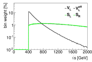
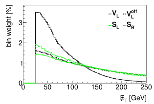
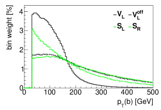
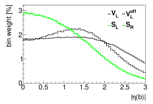
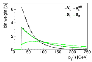
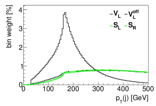
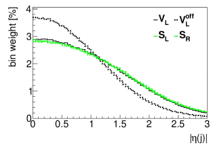
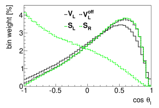
Figure 2: Normalized $s$ channel distributions at parton level.

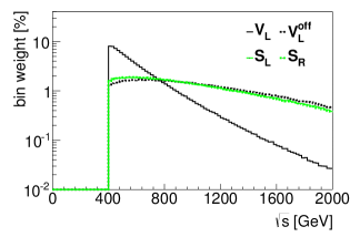
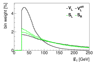
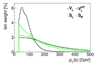
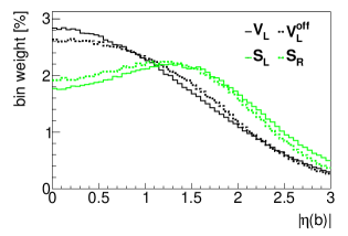
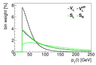
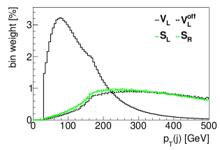
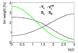
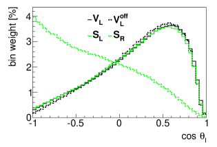
Figure 3: Normalized $t$ channel distributions at parton level.

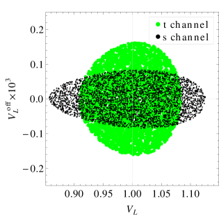
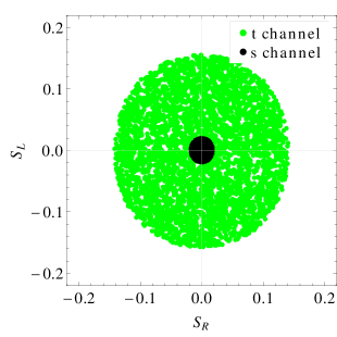
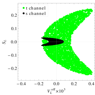
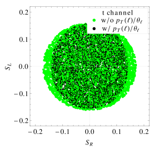
Figure 4: Channel specific sensitivities in various coupling planes (top and bottom left) and effect of the $S_{R}$ sensitive observables $p_{T}(\ell)$ and $\cos\theta_{\ell}$ in the $t$ channel (bottom right) at parton level.

Finally, in Fig. 4 we compare the $1\sigma$ contours in the two different production channels at parton level, finding that the $s$ channel generally is much more sensitive to the contact couplings than the $t$ channel. This could be expected from the fact that the $s$ channel is maximally sensitive to the high energy tails of the contact interactions, which is particularly evident in the $S_{L}$-$S_{R}$ plane. The fact that the $s$ channel sensitivity to the scalars supersedes the $t$ channel one by roughly an order of magnitude is not only due to more sensitive shapes, but also due to the much larger overall sizes of the matrix elements, a feature which is not displayed in the normalized shapes of Fig. 4. Note that either the different relative sensitivities in the two channels when comparing the scalar plane to the vector plane or the sign change in the $V_{L}$-$V_{L}^{\text{off}}$ interference (cf. Fig. 4 bottom left) can in principle be used to distinguish $V_{L}^{\text{off}}$ from the scalar couplings by a separate analysis of each individual channel. However, the detector level analysis below will address the question whether the production channels can be separated at all with a sufficient purity. Moreover, if one compares the sensitivity to $V_{L}$ with the one obtained in Bach and Ohl (2012), there is obviously no significant gain from the binned analysis: in fact, this is no surprise, since $V_{L}$ only sets the overall normalization of the SM shapes but does not distort them, while on the other hand, the sensitivity to $V_{L}^{\text{off}}$ increases by more than 2 orders of magnitude. Finally, as also illustrated in Fig. 4, the observables $p_{T}(\ell)$ and $\cos\theta_{\ell}$ are indeed specifically sensitive to $S_{R}$, potentially amounting to a $\sim 20\,\mathrm{\%}$ gain on the $S_{R}$ limit with respect to the $S_{L}$ one, and could hence be employed to distinguish any anomalous right-handed part in single top production. To conclude this paragraph, one may state that the LHC sensitivity reach to the four-fermion interactions vitally depends on the capability to cleanly separate the $s$ channel signal at the detector level, a task that shall be addressed now in more detail.

III.3 Detector level

Detector effects are being accounted for by processing the SM samples with pythia 6 Sjostrand et al. (2006) and Delphes Ovyn et al. (2009); de Favereau et al. (2013) to obtain detector level samples, where in the latter we assume by default a global $b$-tagging efficiency of $60\,\mathrm{\%}$ with corresponding impurity from charm and light flavors taken from Aad et al. (2009). On these samples the following final state selections are applied: in addition to an isolated lepton with $p_{T}>25\,\mathrm{GeV}$ and missing transverse energy $\not{E}_{T}>25\,\mathrm{GeV}$, the selection criteria for the two final state signatures are, respectively,

1. $s$ channel or “$tb$” selection: exactly two $b$ tagged jets with $p_{T}>30\,\mathrm{GeV}$, and neither central nor forward light jets with $p_{T}>15\,\mathrm{GeV}$. Furthermore, the top momentum is reconstructed from one of the $b$ jets together with the charged lepton and $\not{E}_{T}$ (identified with the neutrino $p_{T}$), by applying the on-shell constraint $\left(p_{\ell}+p_{\nu}\right)^{2}=m_{W}^{2}$ and picking the smaller of the two solutions for the longitudinal component of $p_{\nu}$. The resulting top mass is required to be within 150 and $225\,\mathrm{GeV}$.

2. $t$ channel or “$tj$” selection: one or more $b$ jets with $p_{T}>30\,\mathrm{GeV}$ (one of them reconstructing the top together with the leptons as before), one light forward jet with $p_{T}>50\,\mathrm{GeV}$ and $0<\left|\eta\right|<3$ and at most one additional light central jet, which may have $p_{T}<30\,\mathrm{GeV}$ only.

Finally, the overall invariant mass of the event given by the reconstructed top and the hardest spectator jet must be $m_{tj}>400\,\mathrm{GeV}$. Note that the universal partonic acceptance cuts applied on the matrix elements, Eq. (13), have been deliberately designed such that they contain the entire phase space regions of the final state selections stated here for any of the two channels.

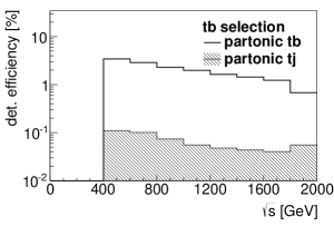
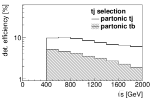
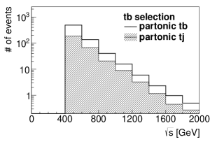
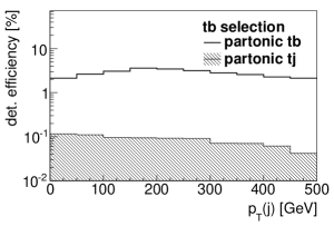
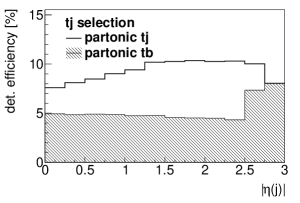
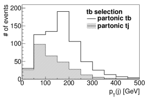
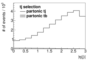
Figure 5: The detector efficiency matrix entries $\epsilon_{ij}$ ($tb$ selection on each partonic input process left, $tj$ selection right) and resulting binned event numbers corresponding to $\int\!L=100\,\mathrm{fb^{-1}}$, for various kinematic distributions.

Within each of the two selections, we fill the histograms of the kinematic observables introduced at parton level in Eq. (16). All histograms are then rebinned appropriately to match parton and detector levels, so that the efficiency matrix $\epsilon_{ij}$ is given by the ratio of detector level events in selection $i$ over the partonic ones in production channel $j$, for each bin in the analysis. However, there remains a subtlety in the approach: $b$ tagging should be part of the detector response, so in a strict sense one cannot use flavor information at parton level. On the other hand, the spectator kinematics (a $b$ jet in the $s$ channel, respecitvely, a light jet in the $t$ channel) is a vital property of the final states, so it should be accounted for in the analysis, including off-diagonal elements of the detector response. This is resolved by leaving the spectator jet untagged in both channels after the final state selection (i.e. demanding only one or exactly two $b$ jets in the $t$, respecitvely, $s$ channel). The spectator, globally denoted “$j$”, is then simply identified in both selections as the hardest jet remaining in the event after the $b$ tagged one reconstructing the top momentum has been removed.

The result of the procedure is displayed in Fig. 5 for some characteristic observables in each final state, showing the binned entries of the detector efficiency matrix $\epsilon_{ij}$ in percent as well as resulting absolute event counts at detector level, normalized to the reference luminosity $\int\!L=100\,\mathrm{fb^{-1}}$. Figure 5 illustrates how the $s$ channel selection efficiently suppresses the $t$ channel sample, whereas the $t$ channel selection is less restrictive against an $s$ channel admixture. However, this high $s$ channel purity is mandatory because the total cross sections deviate by more than an order of magnitude in the two production channels, so that the $s$ channel still suffers from sizable $t$ channel pollution, as reflected in the total event numbers resolved by the partonic sample input. On the other hand, for the same reason the $t$ channel selection is indeed very clean, despite the fact that the efficiencies of the partonic input samples only deviate roughly by a factor of two. In the last bin of the $|\eta(j)|$ spectator histogram, the $tj$ selection efficiencies even become identical on both inputs, which is actually a consistency requirement: since $b$ tagging does not work any more above $|\eta|\gtrsim 2.5$, the hard $b$ in the $s$ channel mimics the hard light jet in the $t$ channel and hence passes the respective selection criteria with practically the same efficiency as an original partonic $tj$ event.

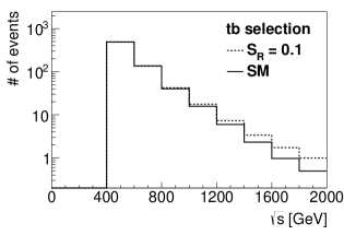
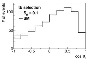
Figure 6: Detector level histograms of $\sqrt{s}$ (left) and $\cos\theta_{\ell}$ (right) after $tb$ selection at the reference point $S_{R}=0.1$ (event numbers normalized to $\int\!L=100\,\mathrm{fb^{-1}}$).

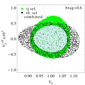
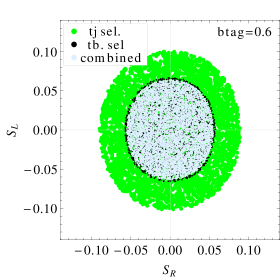
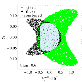
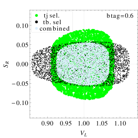
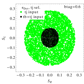
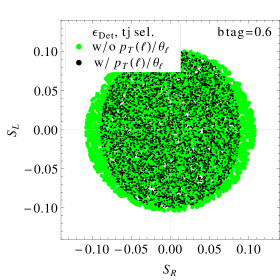
Figure 7: The $1\sigma$ limits resolved by final state selections at detector level in various coupling planes, always setting the other couplings to their SM values (top and center rows). The bottom row shows additional features in the $S_{L}$-$S_{R}$ plane (see text).

Going on now to the results based on the binned likelihood test which are summarized in Fig. 7 (cf. the Appendix for systematic effects from variations of various analysis parameters), let us first compare the $1\sigma$ bounds resolved by final state selections displayed in the top row with the ones on the partonic level (top row in Fig. 4). It is no surprise that generally the limits tend to get worse at the detector level, especially in the $s$ channel which gets considerably diluted by $t$ channel events. However, in the scalar plane (top right in Fig. 7) one observes the counterintuitive result that the $t$ channel sensitivity appears to increase at the detector level, but in truth this is also explained by the selection impurity, however tiny in the $t$ channel at the SM point. Once the scalar NP couplings are turned on, the $s$ channel events also significantly populate the $t$ channel bins at the detector level, due to the fact that the integrated NP cross sections differ by orders of magnitude, as already pointed out in the parton level discussion above. A simple cross-check is given by switching off the $s$ channel partonic input to the $t$ channel selection, as was done in the bottom left plot in Fig. 7, highlighting that the $t$ channel sensitivity to the scalar couplings is indeed governed by the $s$ channel admixture. It follows that the best limits on the scalar couplings are entirely driven by the $s$ channel sensitivity, numerically amounting to $|S_{L}|\lesssim 0.075$, respecitvely, $|S_{R}|\lesssim 0.065$ in this study (varying all four couplings independently), which translates into a sensitivity on the underlying Wilson coefficients already of $\mathcal{O}(0.1\text{--}1)$ when the naive NP scale estimate $\Lambda\sim 3\,\mathrm{TeV}$ is employed. The enhanced sensitivity to the right-handed part is again due to the discriminative observables $p_{T}(\ell)$ and $\cos\theta_{\ell}$ that were already discussed at the parton level. To further quantify this observation, in Fig. 8 we show the relative $\chi^{2}$ value $\chi^{2}|_{p_{T}(\ell),\cos\theta_{\ell}}/\chi^{2}_{\text{tot}}$ collected in these observables inside the $1\sigma$ region obtained from the $tj$ selection. One finds that along the $S_{R}$ direction the $\chi^{2}$ is indeed dominated ($\gtrsim 50\,\mathrm{\%}$) by $p_{T}(\ell)$ and $\cos\theta_{\ell}$, while along $S_{L}$ the contribution is moderate ($\lesssim 10\,\mathrm{\%}$). For illustration, Fig. 6 shows the effect of an NP contribution corresponding to $S_{R}=0.1$, which is in tension with the SM at the $\sim 3\sigma$ level in our analysis (varying all couplings), to the $tb$ channel selection.

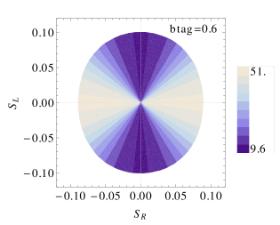
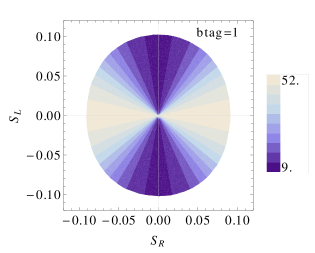
Figure 8: Contribution from the helicity sensitive observables $p_{T}(\ell)$ and $\cos\theta_{\ell}$ to the total $\chi^{2}$ value (in percent) inside the $1\sigma$ region from $tj$ selection in the scalar plane.

In the vector plane (top left in Fig. 7), the relative matrix element sizes of the two channels do not deviate that much, so that the sensitivities generally drop at detector level. Varying all four couplings independently, the best limits are obtained by a combination of both channels, numerically resulting in $0.90\lesssim V_{L}\lesssim 1.09$ and $-0.6\lesssim V_{L}^{\text{off}}\times 10^{3}\lesssim 0.55$, the latter being almost exactly 2 orders of magnitude better than the result of Bach and Ohl (2012) and corresponding to a sensitivity on the respective Wilson coefficient of $\mathcal{O}(0.01\text{--}0.1)$ at $\Lambda\sim 3\,\mathrm{TeV}$.

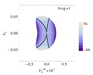
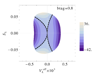
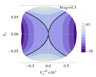
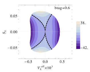
Figure 9: Value of the vector–scalar discriminant $P$ inside the $1\sigma$ region from combination of $tb$ and $tj$ selections in the $V_{L}^{\text{off}}$–$S_{L}$ plane, with varying $b$-tagging setups. The 0-contour is highlighted by black dashed lines.

It remains to address the discrimination of $V_{L}^{\text{off}}$ vs scalar NP contributions. As already hinted in Sec. III.2, this may be achieved by correlating $s$ channel with $t$ channel observations, thus exploiting the $V_{L}$–$V_{L}^{\text{off}}$ interference which switches sign between the channels (cf. bottom left in Fig. 4, respecitvely, center left in Fig. 7). However, as also becomes clear once more from these plots, the final state selections suffer from mutual admixture, essentially governed by the $b$-tagging performance because the main difference of the selections is the tag of the hardest spectator jet. Nonetheless, defining a sign sensitive channel-specific pull

$$P_{k}(\vec{g}) =\sum_{i\in k}\left(\frac{w^{\text{exp}}_{i}-w^{\text{th}}_{i}(\vec{g})}{\delta_{i}}\right)\;,\quad k=s,t\text{ channel}$$ (18)

one can construct a discriminant $P\equiv P_{s}\cdot P_{t}$, which is negative (positive) in a $V_{L}^{\text{off}}$ ($S_{L,R}$) enriched sample. The result is shown in Fig. 9, resolved by various $b$-tagging setups apart from the default one described above, namely perfect tagging (unit efficiency and vanishing impurity) as well as several reference points taken from the characteristic efficiency/impurity curve as estimated in Aad et al. (2009). One observes that while the general correlation between the sign of $P$ and the parameter point $\vec{g}$ is retained, the $b$ tagging affects not only the overall bounds but also the curve of the 0 contour (black dashed lines in Fig. 9) particularly in the positive $V_{L}^{\text{off}}$ hemisphere: this systematics is essential for the accuracy of delimiting the relative admixture of $V_{L}^{\text{off}}$ and $S_{L,R}$. On the other hand, note that the helicity disambiguation shown in Fig. 8 can be carried out entirely in the $t$ channel selection, so that the outcome is stable against the $b$-tagging setup.

In summary, it can be stated that generally both the absolute limits as well as the disambiguation of vector and scalar structures require digging out the tiny amount of $s$ channel events among the $t$ channel ones to a very high precision at the detector level. In the absence of the forward jet tag in the $t$ channel (which would kill the NP signal as illustrated in Fig. 3, bottom left), this reduces to an accurate understanding of the $b$-tagging performance.

IV Conclusions

In this study, we have addressed the impact of including anomalous four-fermion terms $tbf\!f^{\prime}$ into the anomalous top charged-current coupling basis, and point out the possibilities to assess their size and specifically resolve the remaining ambiguities experimentally, by analyzing single top production in the $s$ and $t$ channels at the LHC. The strategy is to employ a binned likelihood test over a set of sensitive kinematic observables, thus exploiting the different kinematic behavior of the four-fermion interactions. In this context, we have first discussed the minimal set of independent minimally flavor violating contact interactions, originally consisting of one vector and eight scalar couplings emerging from dimension six operators. However, after exploiting some kinematic degeneracies, the parameter space is reduced to two scalar couplings $S_{L,R}$ in addition to the vector coupling $V_{L}^{\text{off}}$, while the trilinear $tbW$ coupling $V_{L}\sim V_{tb}$ normalizing the SM part is kept also because of the $V_{L}$–$V_{L}^{\text{off}}$ interference, and the insensitivity of $W$ helicity fractions. Detector effects have been taken into account for each bin, including off-diagonal elements among the $s$ and $t$ channel from selection impurity. It turns out that this mutual signal pollution is crucial for the quality of the resulting bounds, because particularly in the scalar directions the $s$ channel sensitivity exceeds the $t$ channel one by orders of magnitude, with the immediate consequence that any gain in the $s$ channel signal purity is directly reflected in improved limits on the scalars.

Finally, numerical bounds were obtained from the analysis normalized to $\int\!L=100\,\mathrm{fb^{-1}}$ at $\sqrt{s}=14\,\mathrm{TeV}$, illustrating the excellent sensitivity reach, of $\mathcal{O}(0.01\text{--}1)$ on the Wilson coefficients for $\Lambda=3\,\mathrm{TeV}$, to such charged-current contact interactions in single top production. Particularly, the interference in the $V_{L}$-$V_{L}^{\text{off}}$ plane which caused the bounds to leak out to small $V_{L}$ values in correlation with $V_{L}^{\text{off}}$ still allowed by the total cross section analysis of Bach and Ohl (2012) is cleanly cut away here. In terms of disambiguating the various contact couplings in the case that a deviation from the SM should become significant, two differential observables are identified which are sensitive to anomalous right-handed top production, namely the charged lepton momentum $p_{T}(\ell)$ as well as the spin analyzer angle $\cos\theta_{\ell}$, which becomes a clean window to right-handed top production once the values of the spin analyzers are fixed with respect to the trilinear couplings $V_{R}$, respecitvely, $g_{L,R}$ from $W$ helicity fractions. On the other hand, if the experimental signal purities permit it, scalar and vector contributions can potentially be told apart by exploiting the sign change in the $V_{L}$–$V_{L}^{\text{off}}$ interference in the two production channels, which poses an interesting challenge to the LHC experiments for the upcoming high energy, high luminosity run.

*

Appendix A Variation of the analysis setup

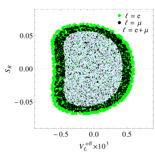
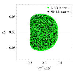
Figure 10: Impact of various parameter variations on the combined $tb$ and $tj$ selection $1\sigma$ bounds in the $V_{L}^{\text{off}}$-$S_{R}$ at detector level (cf. text).

In this short appendix we illustrate the stability of the coupling sensitivities obtained in Sec. III against various variations of the analysis setup. Respective plots are shown in Fig. 10 in the $V_{L}^{\text{off}}$–$S_{R}$ coupling plane containing the vector and one scalar direction for reference, while stating that the observed effects are of the same size also along the other coupling directions. In detail, we have varied (clockwise in Fig. 10, beginning top left) the following:

• the tentative systematic error $\delta_{\text{sys}}$ assumed in Eq. (15), illustrating that the $s$ channel sensitivity driving the scalar bounds is still statistics dominated at the reference luminosity $\int\!L=100\,\mathrm{fb^{-1}}$ (i.e. no visible effect from $\delta_{\text{sys}}$), while the $t$ channel sensitivity contributing to the $V_{L}^{\text{off}}$ bound does change slightly with the value of $\delta_{\text{sys}}$.

• the parameter point from which the detector response matrix $\epsilon$ was inferred, namely once at the SM point and once at the reference point $S_{R}=0.1$ introduced in Sec. III.3. This generically tests the impact of populating the high energy bins on the selection efficiencies and impurities, while also including effects on the helicity-sensitive observables $p_{T}(\ell)$ and $\cos\theta_{\ell}$ (cf. Fig. 6).

• the higher order SM cross section normalization, which is nontrivial despite the normalized bin widths because the $K$ factors, though assumed global in the kinematic sense, are channel specific and hence potentially influence the mutual signal pollution at detector level. For instance, the effect shown in Fig. 10 is mainly along the scalar direction, whose sensitivity is driven by the $s$ channel, which in turn generally has larger $K$ factors than the $t$ channel. Therefore, going from NLO to NNLL slightly improves the sensitivity estimate on the scalars.

• the charged lepton flavor. Note that the discrepancy thus obtained is mainly because of the different detection efficiencies of electrons and muons as modeled by Delphes version 3 de Favereau et al. (2013). For the discussion in Sec. III, both flavors were summed up.

In general, one can state that the systematic effects obtained by these variations are marginal and particularly leave the conclusions of Sec. III.3 unaffected, with the largest uncertainty actually coming from the $b$ tagging which was already discussed in Sec. III.3.

References

- Aad et al. (2008) G. Aad et al. (ATLAS Collaboration), JINST 3, S08003 (2008).
- Aad et al. (2009) G. Aad et al. (ATLAS Collaboration) (2009), [arXiv:0901.0512].
- Chatrchyan et al. (2008) S. Chatrchyan et al. (CMS Collaboration), JINST 3, S08004 (2008).
- Aad et al. (2012a) G. Aad et al. (ATLAS Collaboration), Phys.Lett. B716, 1 (2012a), [arXiv:1207.7214].
- Chatrchyan et al. (2012a) S. Chatrchyan et al. (CMS Collaboration), Phys.Lett. B716, 30 (2012a), [arXiv:1207.7235].
- Chatrchyan et al. (2013a) S. Chatrchyan et al. (CMS Collaboration), Phys.Rev.Lett. 110, 081803 (2013a), [arXiv:1212.6639].
- Aad et al. (2013a) G. Aad et al. (ATLAS Collaboration), Phys.Lett. B726, 88 (2013a), [arXiv:1307.1427].
- Aad et al. (2013b) G. Aad et al. (ATLAS Collaboration), Phys.Lett. B726, 120 (2013b), [arXiv:1307.1432].
- Aad et al. (2011) G. Aad et al. (Atlas Collaboration), Eur.Phys.J. C71, 1577 (2011), [arXiv:1012.1792].
- Aad et al. (2012b) G. Aad et al. (ATLAS Collaboration), JHEP 1205, 059 (2012b), [arXiv:1202.4892].
- Aad et al. (2012c) G. Aad et al. (ATLAS Collaboration), Phys.Lett. B717, 89 (2012c), [arXiv:1205.2067].
- Chatrchyan et al. (2011a) S. Chatrchyan et al. (CMS Collaboration), Eur.Phys.J. C71, 1721 (2011a), [arXiv:1106.0902].
- Chatrchyan et al. (2011b) S. Chatrchyan et al. (CMS Collaboration), JHEP 1107, 049 (2011b), [arXiv:1105.5661].
- Chatrchyan et al. (2012b) S. Chatrchyan et al. (CMS Collaboration), Phys.Rev. D85, 112007 (2012b), [arXiv:1203.6810].
- Chatrchyan et al. (2011c) S. Chatrchyan et al. (CMS Collaboration), Phys.Rev.Lett. 107, 091802 (2011c), [arXiv:1106.3052].
- Aad et al. (2012d) G. Aad et al. (ATLAS Collaboration), Phys.Lett. B717, 330 (2012d), [arXiv:1205.3130].
- Chatrchyan et al. (2012c) S. Chatrchyan et al. (CMS Collaboration), JHEP 1212, 035 (2012c), [arXiv:1209.4533].
- Khachatryan et al. (2014) V. Khachatryan et al. (CMS Collaboration), JHEP 1406, 090 (2014), [arXiv:1403.7366].
- Aad et al. (2012e) G. Aad et al. (ATLAS Collaboration), Phys.Lett. B716, 142 (2012e), [arXiv:1205.5764].
- Chatrchyan et al. (2013b) S. Chatrchyan et al. (CMS Collaboration), Phys.Rev.Lett. 110, 022003 (2013b), [arXiv:1209.3489].
- Chatrchyan et al. (2014) S. Chatrchyan et al. (CMS Collaboration), Phys.Rev.Lett. 112, 231802 (2014), [arXiv:1401.2942].
- Abazov et al. (2013) V. M. Abazov et al. (D0 Collaboration), Phys.Lett. B726, 656 (2013), [arXiv:1307.0731].
- Aaltonen et al. (2014a) T. A. Aaltonen et al. (CDF Collaboration), Phys.Rev.Lett. 112, 231804 (2014a), [arXiv:1402.0484].
- Aaltonen et al. (2014b) T. A. Aaltonen et al. (CDF Collaboration, D0 Collaboration), Phys.Rev.Lett. 112, 231803 (2014b), [arXiv:1402.5126].
- Buchmuller and Wyler (1986) W. Buchmuller and D. Wyler, Nucl.Phys. B268, 621 (1986).
- Arzt et al. (1995) C. Arzt, M. Einhorn, and J. Wudka, Nucl.Phys. B433, 41 (1995), [arXiv:hep-ph/9405214].
- Gounaris et al. (1996) G. Gounaris, M. Kuroda, and F. Renard, Phys.Rev. D54, 6861 (1996), [arXiv:hep-ph/9606435].
- Gounaris et al. (1997) G. Gounaris, D. Papadamou, and F. Renard, Z.Phys. C76, 333 (1997), [arXiv:hep-ph/9609437].
- Brzezinski et al. (1999) L. Brzezinski, B. Grzadkowski, and Z. Hioki, Int.J.Mod.Phys. A14, 1261 (1999), [arXiv:hep-ph/9710358].
- Whisnant et al. (1997) K. Whisnant, J.-M. Yang, B.-L. Young, and X. Zhang, Phys.Rev. D56, 467 (1997), [arXiv:hep-ph/9702305].
- Yang and Young (1997) J. M. Yang and B.-L. Young, Phys.Rev. D56, 5907 (1997), [arXiv:hep-ph/9703463].
- Grzadkowski et al. (2004) B. Grzadkowski, Z. Hioki, K. Ohkuma, and J. Wudka, Nucl.Phys. B689, 108 (2004), [arXiv:hep-ph/0310159].
- Aguilar-Saavedra (2009a) J. Aguilar-Saavedra, Nucl.Phys. B812, 181 (2009a), [arXiv:0811.3842].
- Aguilar-Saavedra (2009b) J. Aguilar-Saavedra, Nucl.Phys. B821, 215 (2009b), [arXiv:0904.2387].
- Aguilar-Saavedra (2011) J. Aguilar-Saavedra, Nucl.Phys. B843, 638 (2011), [arXiv:1008.3562].
- Grzadkowski et al. (2010) B. Grzadkowski, M. Iskrzynski, M. Misiak, and J. Rosiek, JHEP 1010, 085 (2010), [arXiv:1008.4884].
- Weinberg (1980) S. Weinberg, Phys.Lett. B91, 51 (1980).
- Gasser and Leutwyler (1984) J. Gasser and H. Leutwyler, Annals Phys. 158, 142 (1984).
- Georgi (1991) H. Georgi, Nucl.Phys. B361, 339 (1991).
- De Rujula et al. (1992) A. De Rujula, M. Gavela, P. Hernandez, and E. Masso, Nucl.Phys. B384, 3 (1992).
- Arzt (1995) C. Arzt, Phys.Lett. B342, 189 (1995), [arXiv:hep-ph/9304230].
- Bach and Ohl (2012) F. Bach and T. Ohl, Phys.Rev. D86, 114026 (2012), [arXiv:1209.4564].
- Fabbrichesi et al. (2014) M. Fabbrichesi, M. Pinamonti, and A. Tonero (2014), [arXiv:1406.5393].
- Aad et al. (2012f) G. Aad et al. (ATLAS Collaboration), JHEP 1206, 088 (2012f), [arXiv:1205.2484].
- Ali and London (1999) A. Ali and D. London, Eur.Phys.J. C9, 687 (1999), [arXiv:hep-ph/9903535].
- Buras et al. (2001) A. Buras, P. Gambino, M. Gorbahn, S. Jager, and L. Silvestrini, Phys.Lett. B500, 161 (2001), [arXiv:hep-ph/0007085].
- D’Ambrosio et al. (2002) G. D’Ambrosio, G. Giudice, G. Isidori, and A. Strumia, Nucl.Phys. B645, 155 (2002), [arXiv:hep-ph/0207036].
- Kilian et al. (2011) W. Kilian, T. Ohl, and J. Reuter, Eur.Phys.J. C71, 1742 (2011), [arXiv:0708.4233].
- Sjostrand et al. (2006) T. Sjostrand, S. Mrenna, and P. Z. Skands, JHEP 0605, 026 (2006), [arXiv:hep-ph/0603175].
- Ovyn et al. (2009) S. Ovyn, X. Rouby, and V. Lemaitre (2009), [arXiv:0903.2225].
- de Favereau et al. (2013) J. de Favereau, C. Delaere, P. Demin, A. Giammanco, V. Lemaître, et al. (2013), [arXiv:1307.6346].
- Glashow et al. (1970) S. L. Glashow, J. Iliopoulos, and L. Maiani, Phys. Rev. D 2, 1285 (1970), URL http://link.aps.org/doi/10.1103/PhysRevD.2.1285.
- Cao et al. (2007) Q.-H. Cao, J. Wudka, and C.-P. Yuan, Phys.Lett. B658, 50 (2007), [arXiv:0704.2809].
- Aguilar-Saavedra (2008) J. Aguilar-Saavedra, Nucl.Phys. B804, 160 (2008), [arXiv:0803.3810].
- Sullivan (2004) Z. Sullivan, Phys.Rev. D70, 114012 (2004), [arXiv:hep-ph/0408049].
- Boos et al. (2006) E. Boos, V. Bunichev, L. Dudko, V. Savrin, and A. Sherstnev, Phys.Atom.Nucl. 69, 1317 (2006).
- Salam and Rojo (2009) G. P. Salam and J. Rojo, Comput.Phys.Commun. 180, 120 (2009), [arXiv:0804.3755].
- Pumplin et al. (2002) J. Pumplin, D. Stump, J. Huston, H. Lai, P. M. Nadolsky, et al., JHEP 0207, 012 (2002), [arXiv:hep-ph/0201195].
- Kidonakis (2010a) N. Kidonakis, Phys.Rev. D81, 054028 (2010a), [arXiv:1001.5034].
- Kidonakis (2011) N. Kidonakis, Phys.Rev. D83, 091503 (2011), [arXiv:1103.2792].
- Kidonakis (2010b) N. Kidonakis, Phys.Rev. D82, 054018 (2010b), [arXiv:1005.4451].
- Falgari et al. (2011) P. Falgari, F. Giannuzzi, P. Mellor, and A. Signer, Phys.Rev. D83, 094013 (2011), [arXiv:1102.5267].
- Campbell and Ellis (2012) J. M. Campbell and R. K. Ellis (2012), [arXiv:1204.1513].
- Jezabek and Kuhn (1994) M. Jezabek and J. H. Kuhn, Phys.Lett. B329, 317 (1994), [arXiv:hep-ph/9403366].
- Aguilar-Saavedra et al. (2007) J. Aguilar-Saavedra, J. Carvalho, N. F. Castro, F. Veloso, and A. Onofre, Eur.Phys.J. C50, 519 (2007), [arXiv:hep-ph/0605190].
- Aguilar-Saavedra and Bernabeu (2010) J. Aguilar-Saavedra and J. Bernabeu, Nucl.Phys. B840, 349 (2010), [arXiv:1005.5382].
- Jezabek (1994) M. Jezabek, Nucl.Phys.Proc.Suppl. 37B, 197 (1994), [arXiv:hep-ph/9406411].
- Czarnecki et al. (1995) A. Czarnecki, M. Jezabek, and J. H. Kuhn, Phys.Lett. B346, 335 (1995), [arXiv:hep-ph/9411282].
- Brandenburg et al. (2002) A. Brandenburg, Z. Si, and P. Uwer, Phys.Lett. B539, 235 (2002), [arXiv:hep-ph/0205023].
- Bernreuther et al. (2004) W. Bernreuther, A. Brandenburg, Z. Si, and P. Uwer, Nucl.Phys. B690, 81 (2004), [arXiv:hep-ph/0403035].
- Mahlon and Parke (2000) G. Mahlon and S. J. Parke, Phys.Lett. B476, 323 (2000), [arXiv:hep-ph/9912458].