Sampling Strategies for Path Planning
under Kinematic Constraints

Abstract

A well-known weakness of the probabilistic path planners is the so-called narrow passage problem, where a region with a relatively low probability of being sampled must be explored to find a solution path. Many strategies have been proposed to alleviate this problem, most of them based on biasing the sampling distribution. When kinematic constraints appear in the problem, the configuration space typically becomes a non-parametrizable, implicit manifold. Unfortunately, this invalidates most of the existing sampling bias approaches, which rely on an explicit parametrization of the space to explore. In this paper, we propose and evaluate three novel strategies to bias the sampling under the presence of narrow passages in kinematically-constrained systems.

1 Introduction

Due to their conceptual simplicity and their efficiency in a large class of problems, probabilistic planners provide de facto the standard solution to the path planning problem [19]. Their simplicity is given by the fact that they only require two basic operations: configuration sampling and connecting nearby configurations. Their efficiency largely depends on the ability to sample in the areas that need to be crossed to connect the start and goal configurations. Thus, the performance of these planners degrades if the solution path needs to cross an area with a relatively low probability of being sampled. Since these areas typically appear when the obstacles heavily restrict the solution path, this issue is commonly known as the narrow passage problem. The prevalent solution to address this problem is to keep the probabilistic planning approach, but to bias the sample distribution with the aim of increasing the number of samples in the problematic areas.

When the problem at hand includes kinematic constraints, the configuration space is typically a non-parametrizable, implicit manifold embedded in the ambient space defined by the variables representing the degrees of freedom of the robot. Kinematic constraints appear quite often in practice, either due to robot’s morphology [22], or to geometric or contact constraints to fulfill during operation [30, 29, 1]. In view of their relevance, several methods for planning taking them into account kinematic constraints have been presented recently [8, 33, 3, 17], but none of them directly addresses the narrow passage problem. The adaptation of the existing strategies to deal with this problem is not straightforward. Most of these strategies implicitly rely on the capability of trivially sampling new configurations and on being able to easily connect nearby samples, typically using linear interpolation. Unfortunately, except for particular families of problems [14] or for problems that can be formulated using distance constraints [27, 26, 15] these two basic procedures become complex when the problem involves kinematic constraints.

This paper shows that path planners for systems with kinematic constraints can also take advantage of sampling bias strategies to deal with the narrow passage problem. With this objective, we propose and evaluate three novel sampling bias strategies with increasing levels of complexity and efficiency.

After analyzing the main sampling bias methods presented in the literature in Section 2, Section 3 describes the three strategies introduced in this paper, Section 4 evaluates them in representative problems and, finally, Section 5 summarizes the contributions and the points deserving further attention.

2 Related Work

The narrow passage problem has concerned researchers in motion planning since the early works on probabilistic planners. Most of the strategies to address this issue are based on biasing the sampling, exploiting information on the obstacle distribution. The problem is to transfer the information from the workspace, where obstacles are defined, to the configuration space, where the planning is carried out.

Some methods concentrate on rigid body path planning [13, 37, 11], where the relation between the workspace and the configuration space is simpler. The extension of some of these methods to articulated robots is possible [23], but local minima can appear in the presence of simultaneous contacts.

Alternative approaches directly operate in the configuration space. Some of them rely on complete representations of either the workspace [28] or the configuration space [24], which limits their scalability. Other approaches are more lightweight. For instance, Gaussian sampling [5] only requires pairs of samples where one of the samples is in collision and the other is not. In this way, samples are only generated near obstacles and, possibly, in narrow passages. This approach, though, needs to directly sample valid configurations. When the problem includes kinematic constraints, the generation of valid configurations is only simple for particular families of problems [14, 15] or for relatively easy problems [38]. Thus, in general, it is complex to adapt Gaussian sampling to the kinematically-constrained case. Approaches that repair the solutions paths found in an environment where the free space has been dilated also require to easily generate valid random configurations [16].

To detect narrow passages, the bridge-test [34] focuses on the generation of pairs of samples in collision where the central point between these samples is collision-free. Even if the configurations could be generated easily, this test implicitly assumes that the linear interpolation between two samples is also a valid configuration, which is not the case when the configuration space is an arbitrary manifold. The assumption is also taken by the approaches that use linear interpolation to displace the random samples toward the medial axis of the free configuration space [20]. Moreover, approaches that use linear dimensionality reduction of the nodes already in the RRT to bias the sampling [10] are also affected by this issue.

The information of the collisions detected while extending an Rapidly-exploring Random Tree (RRT) can be leveraged to bias the sampling [6]. For instance, using this information the dynamic domain of an RRT node can be defined, i.e, the part of the configuration space where it is worth to extend the tree from that node [35, 18]. As we will see, this approach can be adapted to the kinematically-constrained case defining the dynamic domain in the ambient space rather than in the configuration space.

To the best of our knowledge, there is only one previous sampling bias method directly designed for constrained problems [36]. This work, uses a kd-tree to generate samples, an approach that we extend herein and that has been analyzed in detail recently for systems without kinematic constraints [4].

3 Sampling Bias Strategies for Kinematically-Constrained Problems

Let consider a system described by a $n$-dimensional joint ambient space $\mathcal{A}$ and a $k$-dimensional configuration space $\mathcal{X}\subset\mathcal{A}$ implicitly defined by a set of equality constraints

$$\mathcal{X}=\{{\bf x}\in\mathcal{A}\>|\>{\bf F}({\bf x})={\bf 0}\},$$ (1)

with ${\bf F}:\mathcal{A}\rightarrow\mathbb{R}^{n-k}$, $n>k>0$, and where we assume that $\mathcal{X}$ is a smooth manifold everywhere. Let $\mathcal{O}$ be the obstacle region of $\mathcal{X}$, such that $\mathcal{F}=\mathcal{X}\setminus\mathcal{O}$ is the open set of the non-colliding configurations. Let also assume that ${\bf x}_{s}$ and ${\bf x}_{g}$ are the start and goal configurations, both in $\mathcal{F}$. Then, the path planning problem consists of finding a collision free path linking the query configurations while staying in $\mathcal{F}$ i.e. to find a continuous function $\sigma:[0,1]\rightarrow\mathcal{F}$ with $\sigma(0)={\bf x}_{s}$, $\sigma(1)={\bf x}_{g}$. Using a probabilistic planner, a solution path can only be efficiently determined if all the areas of $\mathcal{F}$ to be crossed can be effectively sampled.

Like all the probabilistic planners, general path planners for kinematically-constrained systems have troubles in narrow passages since they sample either with an unspecified distribution [3] or approximately uniformly in $\mathcal{X}$ [17]. Next, we present three strategies that bias the sampling in order to alleviate this problem. The first one is an adaptation of the dynamic domain approach [35]. The second one extends the kd-tree sampling strategy proposed in [36]. Finally, the third strategy exploits the particular characteristics of the AtlasRRT planner introduced in [17].

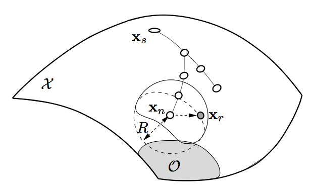
Figure 1: With the dynamic domain technique proposed herein, the sampling domain for nodes near obstacles is restricted to a ball of radius $R$ in the ambient space. Samples in the Voronoi region of these nodes but outside this ball are rejected. In the figure, the obstacle region $\mathcal{O}$ is shown in gray. These problematic areas are not explicitly represented, but detected with RRT extension failures.

3.1 Dynamic Domain

In a standard RRT process, a node is selected for extension if a random sample is drawn in its Voronoi region. For simplicity, the distance to determine the Voronoi regions does not consider the obstacles. However, obstacles can severely limit the area where the tree can actually grow from a given node. The dynamic domain RRT planner reduces the Voronoi area of the nodes for which an RRT extension is truncated due to a collision, i.e., of nodes close to obstacles. The Voronoi region for those nodes is then bounded by a ball of radius $R$. In subsequent iterations, these nodes are extended only if a sample is drawn in the part of the Voronoi region limited by this ball. This strategy outperforms other RRT-like planners in cluttered scenarios because it focuses the efforts on refining problematic areas rather than on performing unsuccessful extensions toward obstacles. Moreover, this sampling strategy reduces the number of collision detection tests, one of the most expensive operations for probabilistic planners.

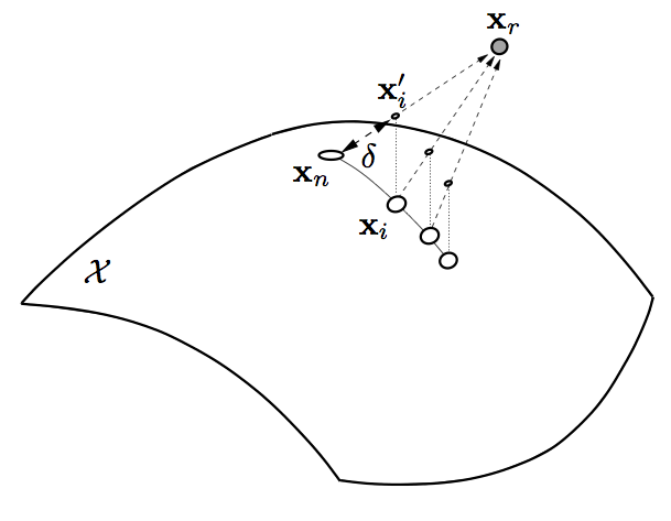
Figure 2: The extension procedure iteratively expands an RRT node $\mathbf{x}_{n}$ towards a random sample $\mathbf{x}_{r}$ in the ambient space $\mathcal{A}$ to obtain a new point $\mathbf{x}_{i}^{\prime}$ that is then projected to obtain a point in $\mathcal{X}$, $\mathbf{x}_{i}$.

Strictly speaking, when the problem includes kinematic constraints, the nearest neighbors and, thus, the dynamic domain should be defined in $\mathcal{X}$. This requires to use the geodesic metric of $\mathcal{X}$, which, for a general manifold, is not available in closed form. In some cases, the geodesic distance can be numerically evaluated [21], but the process is computationally too expensive to be used in a practical planner. The usual solution is to rely on the metric of $\mathcal{A}$ as an approximation to the metric on $\mathcal{X}$. Herein, we propose to use this approximation to adapt the dynamic domain approach to the kinematically-constrained case, defining the balls associated with the RRT nodes in $\mathcal{A}$, as illustrated in Fig. 1. Since $\mathcal{X}$ is assumed to be regular manifold, a ball around a point $\mathbf{x}$ always includes a non-null portion of $\mathcal{X}$. This will be the effective dynamic domain for $\mathbf{x}$. Note that, in general, the distance in $\mathcal{A}$ is lower than the distance in $\mathcal{X}$ and, thus, this approximation can lead to some false positives, i.e., samples that are accepted when they are actually too far form the corresponding RRT node when the motion is restricted to $\mathcal{X}$. These samples produce unnecessary RRT extensions that can reduce the advantage of the dynamic domain approach, but that do not compromise its completeness.

In the dynamic domain approach proposed herein, a procedure to grow RRT branches in $\mathcal{X}$ from samples in $\mathcal{A}$ is necessary. To this end we propose to use the procedure introduced in [3] and illustrated in Fig. 2. With this procedure, a new point $\mathbf{x}_{i}^{\prime}$ is generated by linearly interpolating between the random sample in $\mathcal{A}$, $\mathbf{x}_{r}$, and the nearest node in the RRT, $\mathbf{x}_{n}$,

$$\mathbf{x}_{i}^{\prime}=\mathbf{x}_{n}+\delta\>\frac{\mathbf{x}_{r}-\mathbf{x}_{n}}{\|\mathbf{x}_{r}-\mathbf{x}_{n}\|}\>,$$ (2)

with a small parameter $\delta$. Then a configuration in $\mathcal{X}$, $\mathbf{x}_{i}$, is determined initializing $\mathbf{x}_{i}$ to $\mathbf{x}_{i}^{\prime}$ and updating it with the increments

$$\Delta\mathbf{x}_{i}=-\>\mathbf{J}(\mathbf{x}_{i})^{\!\top}(\mathbf{J}(\mathbf{x}_{i})\>\mathbf{J}(\mathbf{x}_{i})^{\!\top})^{-1}\>\mathbf{F}(\mathbf{x}_{i})\>,$$ (3)

with $\mathbf{J}(\mathbf{x}_{i})$ the Jacobian of $\mathbf{F}$ evaluated at $\mathbf{x}_{i}$. This correction is applied iteratively until $\mathbf{x}_{i}$ is in $\mathcal{X}$, up to the numerical accuracy, or for a maximum number of iterations. In the later case, the projection fails to converge. If successful, the interpolation and projection steps are repeated to continue the RRT branch until an obstacle is found or the expansion gets stalled, i.e., the distance between two consecutive samples in the branch is too small or the projection to $\mathcal{X}$ fails.

Although an adaptive version of the dynamic domain planner exists where parameter $R$ is self-tuned [18], herein we will use a fixed $R$, which will be adjused experimentally to obtain the best performance from this approach.

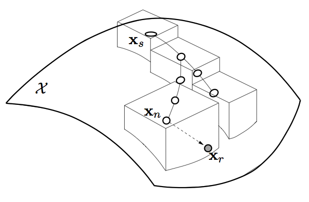
Figure 3: With the kd-tree sampling technique, the kd-tree used to speed up the search for nearest neighbors is also used for sampling. In the figure, the rectangles represent the $r$-bounding rectangles in the leaves of the kd-tree, which bound the area where samples are drawn.

3.2 Kd-tree Sampling

The kd-tree sampling [36] aims at solving a large class of constrained problems where the constraints can be formalized as

$$\|\mathbf{F}(\mathbf{x})\|\leq\varepsilon.$$ (4)

In principle (4) includes (1) when $\varepsilon=0$, but in the original approach $\varepsilon$ is always positive and, thus, it only deals with an approximated version of the problem addressed herein.

In this planner the sampling domain is defined taking advantage of the kd-tree typically used to speed up the nearest neighbor detection. A kd-tree is a hierarchical structure that organizes a set of points in a given space ($\mathcal{A}$ in our case) by recursively partitioning this space. In the internal nodes of the kd-tree, the space is splitted in two sub-domains along a given dimension. If the split point is selected as the median in the split dimension of the points to be organized, the tree is balanced. The tree leaves include the points in the corresponding subdomain of the space.

In this approach, samples are generated in the so-called $r$-bounding rectangles. Such rectangles are the intersection between the subdomain of $\mathcal{A}$ covered by a given leaf and an $n$-dimensional box with two opposite corners

$$\mathbf{x}_{1} =(\min\{x_{i}^{1}\}-r,\ldots,\min\{x_{i}^{n}\}-r)^{\!\top},$$ (5)

$$\mathbf{x}_{2} =(\max\{x_{i}^{1}\}+r,\ldots,\max\{x_{i}^{n}\}+r)^{\!\top},$$ (6)

with $\mathbf{x}_{i}=(x_{i}^{1},\ldots,x_{i}^{n})^{\!\top}\in L$, where $L$ is the set of points in the leaf. The intersection with the subdomain of $\mathcal{A}$ corresponding to the leaf ensures that the $r$-bounding rectangles for different leaves do not intersect.

The internal nodes of the kd-tree only need to add the volumes of the $r$-bounding rectangles in the leaves of the corresponding sub-trees. This information is used to distribute the samples in the sub-trees in the right proportion. Finally, in a leaf, the sampling is uniform in the associated $r$-bounding rectangle. In this way the samples are distributed uniformly in the space covered by all the $r$-bounding rectangles. Fig. 3 shows a mock-up of such rectangles for a set of points in a manifold.

In the original approach, the RRT is extended toward the random sample using linear interpolation as far as the error is below $\varepsilon$. Thus, to avoid errors larger than $\varepsilon$, $r$ must be small. Herein, we propose to combine this sampling strategy with the extension strategy described in the previous section, which always generates samples in $\mathcal{X}$, i.e. with $\varepsilon=0$ up to the numerical accuracy. In this way, $r$ can be set to a larger value, which favors exploration.

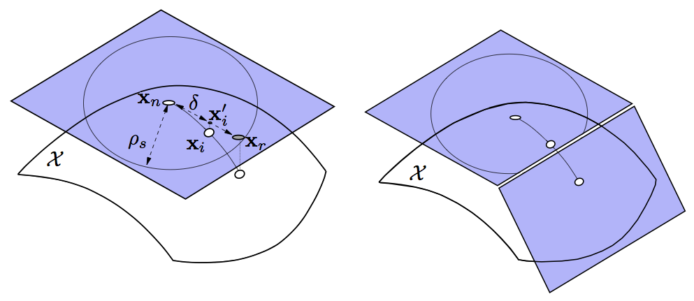
Figure 4: Left: The AtlasRRT samples points in a ball defined in a tangent space of the manifold $\mathcal{X}$. Then, the branches are grown moving in this tangent space and orthogonally projecting to $\mathcal{X}$. Right: When the error or the curvature of the tangent space with respect to $\mathcal{X}$ is above a given threshold, or when a maximum span in a given chart is reached, a new tangent space is generated. This tangent space is properly coordinated with the previous ones, cropping the respective sampling balls.

3.3 Dynamic Domain AtlasRRT

The AtlasRRT [17] does not sample in $\mathcal{A}$, but in a subset of the tangent bundle of $\mathcal{X}$ that is defined as the RRT grows. An orthonormal basis for the tangent space of $\mathcal{X}$ at a given point $\mathbf{x}$ is given by the $n\times k$ matrix, ${\bf\Phi}$, satisfying

$$\left[\begin{array}[]{c}{\bf J}({\bf x})\\ {\bf\Phi}^{\!\top}\end{array}\right]{\bf\Phi}=\left[\begin{array}[]{c}{\bf 0}\\ {\bf I}\end{array}\right],$$ (7)

with ${\bf I}$ the $k\times k$ identity matrix. This tangent space can be seen as a chart that locally parametrizes $\mathcal{X}$ and a collection of such charts forms an atlas of the implicit manifold [12].

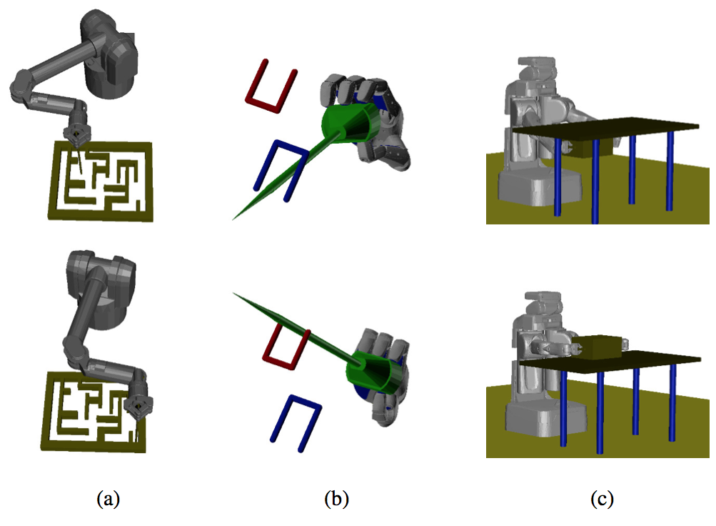
Figure 5: The three benchmarks used in this paper. For each benchmark, the top and bottom pictures correspond to start and goal configurations, respectively. (a) The Barrett arm solving a maze problem. (b) The Schunk anthropomorphic moving a needle in an environment with two U-shaped obstacles. (c) The PR2 service robot moving a box.

To extend an AtlasRRT, a random point $\mathbf{x}_{r}$ is sampled in a ball of radius $\rho_{s}$ in the tangent space of a given chart selected at random. Next, a new RRT branch is grown by first linearly interpolating between $\mathbf{x}_{r}$ and $\mathbf{x}_{n}$, the node in the RRT nearest to $\mathbf{x}_{r}$, using (2) to obtain a point $\mathbf{x}_{i}^{\prime}$ that is then by orthogonally projected to $\mathcal{X}$. This projection is computed solving the system

$$\left\{\begin{array}[]{r}{\bf F}({\bf x}_{i})={\bf 0},\\ {\bf\Phi}_{i}^{\!\top}\>({\bf x}_{i}-{\bf x}_{i}^{\prime})={\bf 0},\end{array}\right.$$ (8)

using a Newton procedure where ${\bf x}_{i}$ is initialized to ${\bf x}_{i}^{\prime}$ and is iteratively updated by the $\Delta{\bf x}_{i}$ increments fulfilling

$$\left[\begin{array}[]{c}{\bf J}({\bf x}_{i})\\ {\bf\Phi}_{i}^{\!\top}\end{array}\right]\Delta{\bf x}_{i}=-\left[\begin{array}[]{c}{\bf F}({\bf x}_{i})\\ {\bf\Phi}_{i}^{\!\top}\>({\bf x}_{i}-{\bf x}_{i}^{\prime})\end{array}\right]\;,$$ (9)

until the error is negligible or for a maximum number of iterations. Fig. 4-left illustrates this procedure. New charts are created when the distance or the curvature of $\mathcal{X}$ with respect to the tangent space being used to extend the RRT exceeds given thresholds or when $\|\mathbf{x}_{i}^{\prime}-\mathbf{x}_{c}\|>\rho$, with $\rho<\rho_{s}$ a given parameter and $\mathbf{x}_{c}$ the point where the chart is tangent to $\mathcal{X}$. This maximum span for the charts improves the regularity of the paving of $\mathcal{X}$. New charts are coordinated with the previous ones to keep track of the area of $\mathcal{X}$ already covered and the corresponding sampling areas are cropped to avoid large overlaps between them, as shown in Fig. 4-right. In subsequent sampling steps, a chart is selected at random and random samples are drawn in the corresponding sampling ball, but those out of the cropped area are rejected.

The natural way to adjust the sampling domain in the AtlasRRT algorithm is to change $\rho_{s}$, which is a critical parameter in the original AtlasRRT planner. Drawing inspiration from [18], we use a global scaling factor that is initialized to 1 and increased by a factor $1+\alpha$, with $\alpha\in(0,1)$ a fixed paremeter, when new RRT branches are grown successfully and decreased by a factor $1-\alpha$ when branches are interrupted due to the presence of obstacles. In any case, $\rho_{s}$ is never lower than $\rho$, which guarantees the continuity between the sampling areas of nearby charts and, thus, the probabilistic completeness of the planner [17].

The global scaling factor can be interpreted as a balance between exploration (when it is set to a large value) and refinement (when its value is low). This balance is automatically adjusted according to the obstacles encountered in the different stages of the RRT expansion. One can say that the difference between [18] and the dynamic domain AtlasRRT, is that the former selects where to limit the exploration while the later decides when to limit it since, at a given moment, the scaling factor globally affects $\rho_{s}$ for all charts. In practice, the global scaling of the sampling areas is more effective than a local chart-based scaling since problematic areas are typically covered by several charts.

4 Experiments and Results

The three sampling bias strategies presented in this paper have been implemented in C and integrated in the CuikSuite [25], a general toolbox for the motion analysis of closed-chain multi-body systems. Figure 5 shows the start and goal configurations for the three benchmarks used in the experimental evaluation, which are taken from [17]. The first benchmark involves the Barrett arm [2] solving a maze problem. The stick moved by the arm has to stay in contact with and perpendicular to the maze plane, without rotating about its axis. In this case, $n$, the dimension of $\mathcal{A}$, is 9 and $k$, the dimension of $\mathcal{X}$, is 3. In the second problem, the Schunk anthropomorphic hand [31] grasps a needle which must be moved getting around a couple of U-shaped obstacles, which introduce local minima in the planning. In this benchmark, $n$ is 23 and $k$ is 5. In the last benchmark, a PR2 robot with fixed base must move a box located under a table to the top of this table, without tilting it. In this case $n$ is 16 and $k$ is 4. In the Barrett arm case, the maze defines a sequence of narrow passages. In the Schunk hand example, the obstacles together with the hand self-collisions and the strict limits of the joints also define several narrow passages. Finally, in the PR2 benchmark there is a problematic area when the box is between the robot and the table, but this passage is relatively wide. Thus, this example is used to evaluate the performance of the proposed sampling strategies when the obstacles do no particularly constraint the solution path. In the experiments reported next, $\delta$ has been set to 0.05, a bidirectional RRT search strategy is used, and the results are averaged over 50 runs on a Intel Core i7 at 2.93 Ghz running Mac OS X. Experiments running for more than 600 seconds are considered a failure and are not taken into account to compute the average results.

	$R$	$t$	CD tests	Col. Bran.	Succ.	Rej.
Barrett arm	2	38	65000	0.92	1	0.96
Schunk hand	0.5	246	118000	0.78	0.5	0.99
PR2	2	18	15000	0.88	1	0.99

Table 1: Results obtained with the dynamic domain strategy.

	$t$	CD tests	Col. Bran.	Succ.
Barrett arm	47	110000	0.99	1
Schunk hand	278	147000	0.83	0.56
PR2	20	16000	0.93	1

Table 2: Results obtained when sampling in the ambient space.

Table 1 shows the results obtained with the dynamic domain technique introduced in Secion 3.1. For each benchmark, the table gives the value for the dynamic domain radius ($R$), the average execution time in seconds ($t$), the number of collision detection tests (CD test), the ratio of RRT branches that end up in a collision (Col. Bran.), the ratio of successful experiments (Succ.), and, finally, the ratio of rejected samples (Rej.). Parameter $R$ has been set to optimize the performance of this approach. As a reference, Table 2, gives the results if the same planning strategy is used, but sampling in $\mathcal{A}$, without the dynamic domain restriction. From Tables 1 and 2, it is clear that the dynamic domain technique reduces the number of collision detection tests and, thus, the overall execution time. Moreover, the ratio of RRT branches ending up in a collision is also reduced, indicating that the dynamic domain RRT focuses more on refinement than on unsuccessful exploration. The reduction of collision detection tests is significant in the first two examples, where the obstacles severely constraint the solution path, and smaller, but still a reduction, in the last problem, which is less constrained. Note, however, that the dynamic domain technique produces a large ratio of rejected samples, which handicaps the approach since the generation of a valid sample can take relatively long.

	$r$	$t$	CD tests	Col. Bran.	Succ.
Barrett arm	0.25	18	50000	0.86	1
Schunk hand	0.5	220	97000	0.75	1
PR2	2	25	21000	0.89	1

Table 3: Results obtained with the kd-tree sampling strategy.

Table 3 shows the results obtained with the kd-tree sampling strategy with the indicated values of $r$. This parameter is set to its optimal value after an exhaustive search. Comparing this table with Table 1, we can see that, in the first two benchmarks, the kd-tree strategy outperforms the dynamic domain technique both in execution time and in reduction of the number of collision detection tests. The main reasons for this superior performance are the increased focus on refinement (as indicated by the reduction in the ratio of branches that end up in a collision) and the lack of rejected samples. The kd-tree sampling strategy is designed to sample directly in the valid sampling area (i.e., in the $r$-bounding rectangles at the leaves of the kd-tree) and, thus rejection is unnecessary. This significantly speeds up this approach. However, sampling only in the $r$-bounding rectangles limits the exploration, which decreases the performance when the obstacles do not particularly constraint the solution path, as it is the case of the PR2 benchmark. The dynamic domain strategy reaches a better trade off between exploration and refinement since it only changes the sampling area for the RRT nodes that are for sure close to obstacles, while the kd-tree sampling strategy reduces the sampling area for all nodes in the RRT. Finally, note that, thanks to its focus on refinement, the kd-tree sampling approach manages to solve the benchmarks in all the cases. This is a remarkable result since the dynamic domain approach is not able to solve the Schunk hand problem in half of the runs.

	$t$	CD tests	Col. Bran.	Succ.	Rej.
Barrett arm	2	10000	0.91	1	0.84
Schunk hand	7	4800	0.95	1	0.64
PR2	1.5	2400	0.89	1	0.64

Table 4: Results obtained with the dynamic domain AtlasRRT.

	$t$	CD tests	Col. Bran.	Succ.	Rej.
Barrett arm	9	37000	0.92	1	0.97
Schunk hand	112	27000	0.97	0.48	0.82
PR2	1	1300	0.97	1	0.76

Table 5: Results obtained with the AtlasRRT.

Table 4 shows the results obtained with the dynamic domain AtlasRRT. In these experiments, $\rho_{s}$ is initialized to 10, $\rho$ and $\alpha$ are set to 1 and 0.1, respectively, and the rest of parameters are the same as those reported in [17] for these benchmarks. As a reference, Table 5 shows the results obtained with the same approach when $\rho_{s}$ is not automatically adjusted, but fixed to 10. In the first two benchmarks, the dynamic domain AtlasRRT outperforms the plain AtlasRRT in execution time, in number of collision detection tests, and in success ratio. In the last benchmark, an aggressive exploration, i.e., fixing $\rho_{s}$ to 10, produces better results. However, the performace degradation introduced by the adaptive sampling radius strategy is minor and acceptable taking into account that this strategy solves the problem of adjusting $\rho_{s}$, which is a major issue in the original AtlasRRT. As a side-effect, the dynamic domain AtlasRRT reduces the rejection ratio for random samples. In the AtlasRRT, the rejected samples are those generated in a given chart, but that are out of the sampling domain due to the coordination with neighboring charts. When $\rho_{s}$ is low, the probability of generating valid samples increases. Finally, note that the dynamic domain AtlasRRT also outperforms the other sampling bias strategies introduced in this paper in all aspects. This superior performance, though, comes at the cost of a higher conceptual and implementation complexity.

5 Conclusions

This paper introduces and evaluates three strategies to deal with the narrow passage problem in systems with kinematic constraints, a relevant problem hardly addressed in the literature so far. The three proposed strategies are based on biasing the sampling distribution and produce improvements with respect to the equivalent planners with unbiased sampling, increasing the ratio of successful runs and reducing the number of collision detection tests and, thus, reducing the execution time. This is achieved by increasing the focus on the refinement of the RRT tree, rather than on its fast expansion, which, in cluttered spaces, mainly leads to collisions. The proposed systems do not rule out exploration, but they reduce it where or when necessary, depending on the approach.

The presented results show that the dynamic domain AtlasRRT strategy is the one that provides better performance, but it is significantly more complex than the two other strategies presented herein. However, we provide an open source implementation of the three approaches with the aim of facilitating their integration in new planners [9].

When the problem involves kinematic constraints, the distance between configurations should be based on the intrinsic metric of the implicit manifold. However, for a general manifold, this metric is complex to compute. Approximated nearest neighbor methods for points on manifolds have been recently introduced [7] and we plan to integrate them in our planner in the near future. Moreover, in this paper, we only considered system with kinematic constraints. In the future, we would like to deal with dynamic constraints too. The presence of these constraints also define an implicit manifold that need to be efficiently explored and, in this exploration, the sampling bias also plays a fundamental role [32].

References

- [1] G. Ballantyne and F. Moll. The da Vinci telerobotic surgical system: Virtual operative field and telepresence surgery. Surgical Clinics of North America, 83(6):1293–1304, 2003.
- [2] Barrett arm web page. http://www.barrett.com.
- [3] D. Berenson, S. S. Srinivasa, and J. J. Kuffner. Task space regions: A framework for pose-constrained manipulation planning. International Journal of Robotics Research, 30(12):1435–1460, 2011.
- [4] J. Bialkowski, M. Otte, and E. Frazzoli. Free-configuration biased sampling for motion planning. In IEEE/RSJ International Conference on Intelligent Robots and Systems, pages 1272–1279, 2013.
- [5] V. Boor, M. H. Overmars, and A. F. van der Stappen. The Gaussian sampling strategy for probabilistic roadmap planners. In IEEE International Conference on Robotics and Automation, volume 2, pages 1018–1023, 1999.
- [6] B. Burns and O. Brock. Single-query motion planning with utility-guided random trees. In IEEE International Conference on Robotics and Automation, pages 3307–3312, 2007.
- [7] R. Chaudhry and Y. Ivanov. Fast approximate nearest neighbor methods for non-Euclidean manifolds with applications to human activity analysis in videos. In European Conference on Computer Vision, pages 735–748, 2010.
- [8] J. Cortés and T. Siméon. Sampling-based motion planning under kinematic loop closure constraints. 6th International Workshop on the Algorithmic Foundations of Robotics, pages 75–90, 2004.
- [9] Cuik project web page. http://www.iri.upc.edu/cuik.
- [10] S. Dalibard and J.-P. Laumon. Linear dimensionality reduction in random motion planning. International Journal of Robotics Research, 30(12):1461–1476, 2011.
- [11] J. Denny, M. Morales, S. Rodriguez, and N. M. Amato. Adapting RRT growth for heterogeneous environments. In IEEE/RSJ International Conference on Intelligent Robots and Systems, pages 1772–1778, 2013.
- [12] M. P. do Carmo. Differential Geometry of Curves and Surfaces. Prentice-Hall, 1976.
- [13] E. Ferré and J.-P. Laumond. An iterative diffusion algorithm for part disassembly. In IEEE International Conference on Robotics and Automation, volume 3, pages 3149–3154, 2004.
- [14] L. Han and N. M. Amato. A kinematics-based probabilistic roadmap method for closed chain systems. In Algorithmic and Computational Robotics. New Directions (WAFR), pages 233–246, 2000.
- [15] L. Han and L. Rudolph. Inverse kinematics for a serial chain with joints under distance constraints. In Robotics: Science and Systems II, pages 177–184, 2006.
- [16] D. Hsu, L. E. Kavraki, J.-C. Latombe, R. Motwari, and S. Sorkin. On finding narrow passages with probabilistic roadmap planners. In International Workshop on Algorithmic Foundations of Robotics, pages 141–153, 1999.
- [17] L. Jaillet and J. M. Porta. Path planning under kinematic constraints by rapidly exploring manifolds. IEEE Transactions on Robotics, 29(1):105–117, 2013.
- [18] L. Jaillet, A. Yershova, T. Siméon, and S. M. LaValle. Adaptive tuning of the sampling domain for dynamic-domain RRTs. In IEEE/RSJ International Conference on Intelligent Robots and Systems, pages 2851–2856, 2005.
- [19] S. M. LaValle. Planning Algorithms. Cambridge University Press, New York, 2006.
- [20] J.-M. Lien, S. L. Thomas, and N. M. Amato. A general framework for sampling on the medial axis of the free space. In IEEE International Conference on Robotics and Automation, volume 3, pages 4439–4444, 2003.
- [21] F. Mémoli and G. Sapiro. Fast computation of weighted distance functions and geodesics on implicit hyper-surfaces. Journal of Computational Physics, 173:730–764, 2001.
- [22] J.-P. Merlet. Parallel Robots. Kluwer, Boston, MA, 2000.
- [23] J. Pan, L. Zhang, and D. Manocha. Retraction-based RRT planner for articulated models. In IEEE International Conference on Robotics and Automation, pages 2529–2536, 2010.
- [24] C. Park, J. Pan, and D. Manocha. Poisson-RRT. In IEEE International Conference on Robotics and Automation, 2014.
- [25] J. M. Porta, L. Ros, O. Bohigas, M. Manubens, C. Rosales, and L. Jaillet. The CUIK suite: Motion analysis of closed-chain multibody systems. IEEE Robotics and Automation Magazine, 2014.
- [26] J. M. Porta, L. Ros, and F. Thomas. Inverse kinematics by distance matrix completion. In Computational Kinematics, pages 1–9, 2005.
- [27] J. M. Porta, F. Thomas, L. Ros, and C. Torras. A branch-and-prune algorithm for solving systems of distance constraints. In IEEE International Conference on Robotics and Automation, pages 342–348, 2003.
- [28] M. Rickert, O. Brock, and A. Knoll. Balancing exploration and exploitation in motion planning. In IEEE International Conference on Robotics and Automation, pages 2812–2817, 2008.
- [29] A. Rodríguez, L. Basaez, and E. Celaya. A relational positioning methodology for robot task specification and execution. IEEE Transactions on Robotics, 24(3):600–611, 2008.
- [30] C. Rosales, L. Ros, J. M. Porta, and R. Suárez. Synthesizing grasp configurations with specified contact regions. International Journal of Robotics Research, 30(4):431–443, 2011.
- [31] Schunk Anthropomorphic Hand web page. http://www.schunk.com.
- [32] A. Shkolnik, M. Walter, and R. Tedrake. Reachability-guided sampling for planning under differential constraints. In IEEE International Conference on Robotics and Automation, pages 2859–2865, 2009.
- [33] M. Stilman. Global manipulation planning in robot joint space with task constraints. IEEE Transactions on Robotics, 26(3):576–584, 2010.
- [34] Z. Sun, D. Hsu, T. Jiang, H. Kurniawati, and J.H. Reif. Narrow passage sampling for probabilistic roadmap planning. IEEE Transactions on Robotics, 21:1105–1115, 2005.
- [35] A. Yershova, L. Jaillet, T. Siméon, and S. M. LaValle. Dynamic-domain RRTs: Efficient exploration by controlling the sampling domain. In IEEE International Conference on Robotics and Automation, pages 3856–3861, 2005.
- [36] A. Yershova and S. M. LaValle. Motion planning for highly constrained spaces. In Robot Motion and Control. Lecture Notes on Control and Information Sciences, volume 396, pages 297–306, 2009.
- [37] L. Zhang and D. Manocha. An efficient retraction-based RRT planner. In IEEE International Conference on Robotics and Automation, pages 3743–3750, 2008.
- [38] Y. Zhang, K. Hauser, and J. Luo. Unbiased, scalable sampling of closed kinematic chains. In IEEE International Conference on Robotics and Automation, pages 2459–2464, 2013.