Measuring the Initial Transient: Reflected
Brownian Motion

Abstract

We analyze the convergence to equilibrium of one-dimensional reflected Brownian motion (RBM) and compute a number of related initial transient formulae. These formulae are of interest as approximations to the initial transient for queueing systems in heavy traffic, and help us to identify settings in which initialization bias is significant. We conclude with a discussion of mean square error for RBM. Our analysis supports the view that initial transient effects for RBM and related models are typically of modest size relative to the intrinsic stochastic variability, unless one chooses an especially poor initialization.

1 Introduction

This paper is concerned with using one-dimensional reflected Brownian motion (RBM) as a theoretical vehicle for studying the initial transient problem. Given that RBM is a commonly used approximation to a wide variety of different queueing models, the initial transient behavior of RBM can be viewed as being representative of a large class of simulation models in which congestion is a key factor.

The stochastic process $X=(X(t):\,t\geq 0)$ is said to be a (one-dimensional) RBM if it satisfies the stochastic differential equation (SDE)

$$dX(t)=-rdt+\sigma dB(t)+dL(t),$$

where $B=(B(t):\,t\geq 0)$ is standard Brownian motion and $L$ is a continuous nondecreasing process that increases only when $X$ is at the origin (so that $I(X(t)>0)dL(t)=0)$. In particular, the process $L$ is a “boundary process” that serves to keep $X$ nonnegative as befits an approximation to a queue. The parameter $-r$ represents the “drift” of the RBM, and $\sigma$ is its “volatility” parameter.

To illustrate the sense in which RBM can be used to approximate a queue, consider a system with a single queue that is being fed by a renewal arrival process in which $\chi$ denotes a generic interarrival time random variable (rv). Customers are served by one of $m$ identical servers, in the order in which they arrive. The service times are independent and identically distributed (iid) across the servers and across the customers, and are also independent of the interarrival times. If $V$ is a rv having the common service time distribution, set $\lambda=1/E\chi,\;\mu=1/EV$ and $\sigma_{A}^{2}=\mathrm{var}\,\chi,\;\sigma_{S}^{2}=\mathrm{var}\,V$. It is well known that if $Z(t)$ is the number-in-system at time $t$, then

$$Z(\cdot)\stackrel{{\scriptstyle\mathscr{D}}}{{\approx}}X(\cdot),$$

where $X$ is an RBM with $r=m\mu-\lambda$ and $\sigma^{2}=\lambda^{3}\sigma_{A}^{2}+m\mu^{3}\sigma_{S}^{2}$, provided that $m\mu-\lambda$ is small (so that the system is in “heavy traffic”) and $t$ is of the order $(m\mu-\lambda)^{-2}$. Here, $\stackrel{{\scriptstyle\mathscr{D}}}{{\approx}}$ means “has approximately the same distribution as”, and the rigorous support rests on a so-called “heavy traffic” limit theorem; see, for example, Iglehart and Whitt (1970).

This paper begins with a discussion of the convergence to equilibrium of RBM (Section 2). It subsequently develops closed-form expressions for various initial transient quantities associated with RBM, distinguishing between “functional” (Section 3) and “distributional” (Section 4) perspectives. These expressions can be used to help plan steady-state/equilibrium simulations of queueing models that can be approximated by RBM as well as to identify settings in which initial bias is significant (Section 5). We conclude by deriving a decomposition of mean square error (MSE) in the setting of RBM (Section 6).

Though only in the context of RBM, the results in this paper are intended develop general insights into the initial transient problem that can be of potentially broader applicability.

2 Convergence to Equilibrium for RBM

It is well-known that if $r>0$, then $X$ has an equilibrium, in the sense that

$$X(t)\Rightarrow X(\infty)$$

as $t\rightarrow\infty$, where $\Rightarrow$ denotes weak convergence. The distribution of $X(\infty)$ is given by $P(X(\infty)\in dx)\stackrel{{\scriptstyle\Delta}}{{=}}\pi(dx)=\eta e^{-\eta x}dx$ for $x\geq 0$, where $\eta\stackrel{{\scriptstyle\Delta}}{{=}}\frac{2r}{\sigma^{2}}$ (see, for example, Harrison (1985) p.94). A key question in the study of the initial transient problem for $X$ is its rate of convergence to equilibrium. One vehicle for studying this question is the well-known formula

$$p(t,\,x,\,y)=\eta e^{-\eta y}\Phi\left(\frac{rt-x-y}{\sigma\sqrt{t}}\right)+\frac{1}{\sigma\sqrt{t}}\phi\left(\frac{-rt+x-y}{\sigma\sqrt{t}}\right)+\frac{1}{\sigma\sqrt{t}}e^{-\eta y}\phi\left(\frac{-rt+x+y}{\sigma\sqrt{t}}\right)$$ (2.1)

for the transition density of $X$; see Harrison (1985) p.49. Here, $p(t,\,x,\,y)dy\stackrel{{\scriptstyle\Delta}}{{=}}P(X(t)\in dy\,|\,X(0)=x)$, $\Phi(x)=P(N(0,\,1)\leq x)$ (where $N(0,\,1)$ denotes a normal rv with mean $0$ and unit variance), and $\phi(x)$ is the density associated with $\phi$. But it is difficult to “read off” the rate of convergence from (2.1).

However, an alternative representation for the transition density of $X$ can be computed. Recall that the rate at which the transition probabilities of a Markov jump process converge to their respective equilibrium probabilities can easily be determined once the eigenvalues and eigenvectors of the rate matrix are known. Something similar can be implemented in the RBM setting. This leads to an alternative representation of the transition density known as the spectral decomposition.

To begin, note that Itô’s formula gives

$$d(e^{-\lambda t}u(X(t))) = -\lambda e^{-\lambda t}u(X(t))dt+e^{-\lambda t}u^{\prime}(X(t))dX(t)+e^{-\lambda t}\frac{u^{\prime\prime}(X(t))}{2}\sigma^{2}dt$$

$$= e^{-\lambda t}((\mathscr{L}u)(X(t))-\lambda u(X(t)))dt+e^{-\lambda t}u^{\prime}(X(t))\sigma dB(t)+e^{-\lambda t}u^{\prime}(X(t))dL(t),$$

where $\mathscr{L}$ is the second order differential operator given by

$$\mathscr{L}\stackrel{{\scriptstyle\Delta}}{{=}}-r\frac{d}{dx}+\frac{\sigma^{2}}{2}\frac{d^{2}}{dx^{2}}.$$

Because $L$ increases only when $X$ is at the origin, $u^{\prime}(X(t))dL(t)=u^{\prime}(0)dL(t)$. Consequently, if $u^{\prime}(0)=0$ and the stochastic integral is integrable,

$$e^{-\lambda t}u(X(t))-\int_{0}^{t}e^{-\lambda s}((\mathscr{L}u)(X(s))-\lambda u(X(s)))ds$$

is a martingale. It follows that if $u$ also satisfies

$$\mathscr{L}u=\lambda u$$ (2.2)

(subject to $u^{\prime}(0)=0$), then $E_{x}u(X(t))=e^{\lambda t}u(x)$ for $t,\,x\geq 0$, where $E_{x}(\cdot)\stackrel{{\scriptstyle\Delta}}{{=}}E(\cdot\,|\,X(0)=x)$. If $\lambda<0$, sending $t\rightarrow\infty$ allows us to conclude that $Eu(X(\infty))=0$, and the rate of convergence of $E_{x}u(X(t))$ is exponentially fast with associated rate parameter $\lambda$.

Remark: This makes clear that the rate of convergence of $E_{x}f(X(t))$ to $Ef(X(\infty))$ often depends on the choice of $f$.

For each $\lambda\in\mathbb{R}$, there exists a nontrivial solution (unique up to multiplicative constants) to (2.2), which can be found by direct computation. However, according to Linetsky (2005), the spectrum (in the operator theoretic sense) consists only of $\lambda=0$ and $\lambda\leq-\gamma$, where $\gamma\stackrel{{\scriptstyle\Delta}}{{=}}r^{2}/(2\sigma^{2})$. As a consequence, the distance between the top two points in the spectrum, namely $0$ and $-\gamma$, is equal to $\gamma$. This distance is known, in the Markov process literature, as the spectral gap of $X$.

For $\lambda\in(-\infty,-\gamma)$, let

$$u_{\lambda}(x)\stackrel{{\scriptstyle\Delta}}{{=}}e^{\frac{rx}{\sigma^{2}}}\left(s(\lambda)\cos\left(\frac{s(\lambda)x}{\sigma^{2}}\right)-r\sin\left(\frac{s(\lambda)x}{\sigma^{2}}\right)\right).$$

where $s(\lambda)=\sigma\sqrt{-2(\lambda+\gamma)}$. There is a standard “recipe” for constructing the transition density for reversible diffusion processes (of which RBM is one) that can be found, for example, on p.332 of Karlin and Taylor (1981). When specialized to the RBM setting, one obtains the spectral decomposition for $p(t,\,x,\,y)$, namely

$$p(t,\,x,\,y) = \frac{2r}{\sigma^{2}}e^{-\frac{2r}{\sigma^{2}}y}+\frac{2}{\pi\sigma^{2}}e^{-\frac{r(y-x)}{\sigma^{2}}-\frac{r^{2}t}{2\sigma^{2}}}$$

$$\qquad\cdot \int_{0}^{\infty}\frac{e^{-\frac{v^{2}t}{2\sigma^{2}}}}{v^{2}+r^{2}}\left(v\cos\left(\frac{vx}{\sigma^{2}}\right)-r\sin\left(\frac{vx}{\sigma^{2}}\right)\right)\left(v\cos\left(\frac{vy}{\sigma^{2}}\right)-r\sin\left(\frac{vy}{\sigma^{2}}\right)\right)dv$$

$$= \eta e^{-\eta y}-\frac{1}{2\pi r}\cdot\int_{-\infty}^{-\gamma}e^{\lambda t}u_{\lambda}(x)u_{\lambda}(y)\frac{1}{s(\lambda)\lambda}\eta e^{-\eta y}d\lambda$$

(see Linetsky (2005)). We thus find that, for $f$ appropriately integrable,

$$E_{x}f(X(t))=Ef(X(\infty))-\frac{1}{2\pi r}\cdot\int_{-\infty}^{-\gamma}e^{\lambda t}u_{\lambda}(x)\langle f,\,u_{\lambda}\rangle\frac{1}{s(\lambda)\lambda}d\lambda,$$ (2.3)

where

$$\langle f,\,u_{\lambda}\rangle\stackrel{{\scriptstyle\Delta}}{{=}}\int_{0}^{\infty}f(y)u_{\lambda}(y)\eta e^{-\eta y}dy.$$

The spectral representation (2.3) makes clear that the spectral gap $\gamma$ is precisely the exponential rate constant governing the rate at which $E_{x}f(X(t))$ converges to $Ef(X(\infty))$. Furthermore, when $t$ is large, it is primarily the “projection” of $f$ onto $u_{-\gamma}$ (i.e. the magnitude of $\langle f,\,u_{\lambda}\rangle$) that determines the magnitude of $E_{x}f(X(t))-Ef(X(\infty))$ (given that the integral is largely determined by the integrand’s contribution from a neighborhood of $\lambda=-\gamma$).

3 The Initial Transient Effect

Given a performance measure $f$, we have studied in Section 2 the rate of convergence of $E_{x}f(X(t))$ to its equilibrium value $Ef(X(\infty))$. Our goal here is to compute the magnitude of the initial transient effect, assuming that no deletion is implemented. This can inform our decision as to how serious the initial transient effect is, and whether/how deletion is warranted. Because the typical estimator used to compute an equilibrium quantity in a simulation context is a time-average, the effect of the initial transient in the steady-state simulation setting is, in some sense, an integrated version of the theory of Section 2.

To compute the effect of the initial transient, note that if $h$ is twice continuously differentiable with $h^{\prime}(0)=0$, then Itô’s formula yields

$$dh(X(t))=(\mathscr{L}h)(X(t))dt+h^{\prime}(X(t))\sigma dB(t).$$

It follows that if the stochastic integral is integrable and $\mathscr{L}h=-f_{c}$ (with $f_{c}(x)=f(x)-Ef(X(\infty))$ for $x\geq 0$), then

$$M(t)\stackrel{{\scriptstyle\Delta}}{{=}}h(X(t))+\int_{0}^{t}f_{c}(X(s))ds=\int_{0}^{t}h^{\prime}(X(s))\sigma dB(s)$$

is a martingale, from which we conclude that

$$\int_{0}^{t}E_{x}f_{c}(X(s))ds=h(x)-E_{x}h(X(t)).$$

In view of our discussion in Section 2, we expect that

$$E_{x}h(X(t))=Eh(X(\infty))+O(e^{-\gamma t})$$

as $t\rightarrow\infty$, where $O(a(t))$ represents a function for which $O(a(t))/a(t)$ remains bounded as $t\rightarrow\infty$. Thus

$$E_{x}\frac{1}{t}\int_{0}^{t}f(X(s))ds=Ef(X(\infty))+\frac{1}{t}h_{c}(x)+O(e^{-\gamma t})$$

as $t\rightarrow\infty$, where $h_{c}(x)=h(x)-Eh(X(\infty))$. Hence, the constant $h_{c}(x)$ expresses (up to an exponentially small order) the bias of the estimator $t^{-1}\int_{0}^{t}f(X(s))ds$ induced by the initial transient.

We now turn to computing $h_{c}(x)$. The solution $h$ to Poisson’s equation

$$(\mathscr{L}h)(x)=-f_{c}(x),\;\;x\geq 0$$

$$h^{\prime}(0)=0,\;\;h(0)=0$$

is given by

$$h(x)=-\frac{1}{r}\int_{0}^{x}f_{c}(y)(e^{-\eta(y-x)}-1)dy,$$

from which we can conclude that

$$h_{c}(x)=-\frac{1}{r}\int_{0}^{x}f_{c}(y)\left(e^{-\eta(y-x)}-1\right)dy+\frac{2}{\sigma^{2}}\int_{0}^{\infty}\int_{0}^{x}f_{c}(y)(e^{-\eta y}-e^{-\eta x})dydx.$$ (3.1)

Example 3.1.

For $f(x)=x$,

$$h_{c}(x)=\frac{x^{2}}{2r}-\frac{\sigma^{4}}{4r^{3}}.$$

Example 3.2.

For $f(x)=x^{2}$,

$$h_{c}(x)=\frac{x^{3}}{3r}+\frac{\sigma^{2}x^{2}}{2r^{2}}-\frac{\sigma^{6}}{2r^{4}}.$$

Example 3.3.

For $f(x)=e^{\theta x}$ (with $\theta<\eta$),

$$h_{c}(x)=\frac{-\theta^{2}\sigma^{4}+4r^{2}\left(-\theta x+e^{\theta x}-1\right)+2\theta r\sigma^{2}\left(\theta x-e^{\theta x}+1\right)}{\theta r\left(\theta\sigma^{2}-2r\right)^{2}}.$$

Example 3.4.

For $f(x)=I(x>b)$, where $I(\cdot)$ is the indicator function,

$$h_{c}(x)=\begin{cases}\frac{e^{-\frac{2br}{\sigma^{2}}}\left(\sigma^{2}\left(e^{\frac{2rx}{\sigma^{2}}}-1\right)-2r(b+x)\right)}{2r^{2}}&x<b\\ \frac{e^{-\frac{2br}{\sigma^{2}}}\left(e^{\frac{2br}{\sigma^{2}}}\left(-2br+2rx+\sigma^{2}\right)-2r(b+x)-\sigma^{2}\right)}{2r^{2}}&x\geq b.\end{cases}$$

Given the performance measure $f$, the functional unconditional initial transient effect (UNITE) measure is given by

$$\beta_{f}(\mu)=\left|\int_{0}^{\infty}h_{c}(x)\mu(dx)\right|$$

for a given initial distribution $\mu$, while the functional conditional initial transient effect (CITE) measure is defined by

$$\tilde{\beta}_{f}(\mu)=\int_{0}^{\infty}\beta_{f}(\delta_{x})\mu(dx),$$

where $\delta_{x}(\cdot)$ is a unit point mass distribution at $x$; see Wang and Glynn (2014) for a more detailed discussion of these measures. Note that in a single replication setting, the initial transient effect is determined by the random placement of $X(0)$, so that averaging the effect over the initial distribution $\mu$ (as in CITE) seems reasonable. Given this viewpoint, it is then appropriate to view $\tilde{\beta}_{f}(\pi)$ as a benchmark against which $\tilde{\beta}_{f}(\mu)$ for other initializations $\mu$ can be compared. (After all, initializing with $\pi$ makes $X$ a stationary process in which no initial transient is present.)

In particular, we can now separate the state space into “good states” and “bad states”, depending on whether $\beta_{f}(\delta_{x})\leq c\tilde{\beta}_{f}(\pi)$ for the state $x$ or not, where $c$ is a given constant. For example, for $c=1$, the good states are all those states $x$ for which $\beta_{f}(\delta_{x})$ is smaller than the CITE measure associated with $\pi$. Of course, the set of good states is sensitive to the choice of $c$. Hence, it is of interest to study the dependence of the set of good states on the parameter $c$; see Figure 1 below. We note that the notion of good state is related to the “typical state” idea introduced by Grassmann (2011) and Grassmann (2014).

For $f(x)=x$, the set of good states $\mathscr{G}(r,\,\sigma^{2};\,c)\stackrel{{\scriptstyle\Delta}}{{=}}\{x:\,\beta_{f}(\delta_{x})\leq c\tilde{\beta}_{f}(\pi)\}$ is given by

$$\mathscr{G}(r,\,\sigma^{2};\,c) = \left\{x:\,\left|\frac{x^{2}}{2r}-\frac{\sigma^{4}}{4r^{3}}\right|\leq c\left(\frac{(1+\sqrt{2})e^{-\sqrt{2}}\sigma^{4}}{2r^{3}}\right)\right\}$$

$$= \left\{x:\,\left|\frac{1}{2}\left(\frac{x}{EX(\infty)}\right)^{2}-1\right|\leq 2(1+\sqrt{2})ce^{-\sqrt{2}}\right\}.$$

For this performance measure, $\mathscr{G}(r,\,\sigma^{2};\,c)=EX(\infty)\mathscr{G}(1,\,2;\,c)$, so it suffices to graph $\mathscr{G}(r,\,\sigma^{2})\stackrel{{\scriptstyle\Delta}}{{=}}\{(x,\,c):\,x\in\mathscr{G}(r,\,\sigma^{2};\,c),\;c\geq 0\}$ only for $EX(\infty)=1$; the resulting graph can be found below. Note that for $c=1$, the set of good states already covers $[0,\,2.09]$, so that the set of initial values providing single-replication bias characteristics roughly comparable to that associated with initializing under $\pi$ is quite robust (in fact, more than twice the mean).

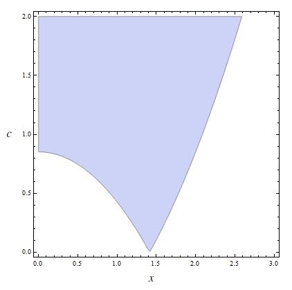
Figure 1: Plot of Good States: $EX(\infty)=1$

4 The Distributional Initial Transient

The convergence of $X(t)$ to $X(\infty)$ involves the entire distribution of $X$ (as opposed to only the convergence of $E_{x}f(X(t))$ for a single performance measure $f$), so that much of the probability literature is concerned with the rate of convergence at which the distribution of $X(t)$ approaches that of $X(\infty)$. In fact, one commonly used measure for judging the rate of convergence to equilibrium is the weighted total variation norm defined by

$$\sup_{|f|\leq w}|E_{\mu}f(X(t))-Ef(X(\infty))|$$

for a given weight function $w:\,\mathbb{R}_{+}\rightarrow\mathbb{R}_{+}$.

By analogy, with the discussion of Section 3, it is natural to study the distributional UNITE measure given by

$$\beta(\mu)\stackrel{{\scriptstyle\Delta}}{{=}}\sup_{|f|\leq w}\beta_{f}(\mu)$$

and the distributional CITE measure defined by

$$\tilde{\beta}(\mu)\stackrel{{\scriptstyle\Delta}}{{=}}\int_{0}^{\infty}\beta(\delta_{x})\mu(dx).$$

In view of the calculation of Section 3, specifically (3.1), it is evident that

$$\beta_{f}(\delta_{x})=\left|\int_{0}^{\infty}f(y)\frac{1}{r}m(\eta x,\,\eta y)dy\right|,$$

where

$$m(u,\,v)=\begin{cases}1-(u+v)e^{-v}&0\leq v\leq u,\\ e^{-(v-u)}-(u+v)e^{-v}&v>u.\end{cases}$$

According to Pollard (2002) p.60,

$$\beta(\delta_{x})=\int_{0}^{\infty}\frac{1}{r}|m(\eta x,\,\eta y)|w(y)dy.$$

Hence, if $w(y)=y^{p}$ for $p\geq 0$,

$$\beta(\delta_{x}) = \frac{1}{r}\eta^{-p-1}\int_{0}^{\infty}v^{p}|m(\eta x,\,v)|dv$$

and

$$\tilde{\beta}(\pi)=\frac{1}{r}\eta^{-p-1}\int_{0}^{\infty}\int_{0}^{\infty}v^{p}|m(u,\,v)|dve^{-u}du.$$

So, as in Section 3, we can analogously define the set of “good states” as

$$\mathop{\mathscr{H}(r,\,\sigma^{2};\,c)} \stackrel{{\scriptstyle\Delta}}{{=}} \{x:\,\beta(\delta_{x})\leq c\tilde{\beta}(\pi)\}$$

$$= EX(\infty)\mathop{\mathscr{H}(1,\,2;\,c)},$$

so that $\mathop{\mathscr{H}(r,\,\sigma^{2};\,c)}$ again scales similarly as does the set $\mathop{\mathscr{G}(r,\,\sigma^{2};\,c)}$ of Section 3, due to the homogeneity of $w(y)=y^{p}$. (For the function $w(y)=e^{\theta y}$, such a scaling relationship does not hold.)

By numerically computing $\tilde{\beta}(\pi)$ (via a numerical integration of $\beta(\delta_{x})$ against $\pi$), the graph of the set $\mathscr{H}(1,\,2)\stackrel{{\scriptstyle\Delta}}{{=}}\{(x,\,c):\,x\in\mathop{\mathscr{H}(1,\,2;\,c)},\;c\geq 0\}$ can be determined. In particular, it is computed below for $w(x)\equiv 1$; see Figure 2. Unlike the set $\mathscr{G}(1,\,2)$ of Section 3, it does not touch the $x$-axis. This is not surprising, because in the functional setting of Section 3, it will often be the case that the bias is monotone in the initial state. For example, for nondecreasing $f$, the stochastic monotonicity of RBM ensures that the bias will be negative for small values of $x$, and positive for large values of $x$, yielding (using a continuity argument) the existence of an intermediate $x$ at which $\beta_{f}(\delta_{x})=0$. On the other hand, in the distributional setting, $\beta(\delta_{x})$ involves looking at the largest possible bias over a large class of functions $f$, and there typically will be no initial $x$ at which $\beta(\delta_{x})$ will vanish.

We further note that the shape of $\mathscr{H}(1,\,2)$ is quite different than that of $\mathscr{G}(1,2)$. For example, the minimizer of $\beta(\delta_{x})$ as a function of $x$ is achieved at a point $x^{*}$ that is smaller than that of $\beta_{f}(\delta_{x})$ for $f(x)=x$. This occurs because $\beta(\delta_{x})$ is defined in terms of the bias of bounded functions, while the set $\mathscr{G}(1,2)$ of Section 3 was computed for the identity mapping (which is unbounded). In computing the expectation of such a performance measure, it is advantageous to initialize the process at a larger value, because such an initialization will lead to higher likelihood paths that will quickly sample the large state values that typically contribute the most to the expectation of the performance measure. We further note that the set of good $x$’s associated with $\mathscr{H}(1,\,2)$ is a bit smaller than that of Section 3 (in part, because $\mathscr{H}(1,\,2)$ involves a worst case bias, where as $\mathscr{G}(1,\,2)$ is determined only by a single function $f$). Nevertheless, the set of good states, with values of $\beta(\delta_{x})$ of a magnitude less than or equal to that associated with initializing under the equilibrium distribution (i.e., $\tilde{\beta}(\pi)$), is large, and includes all the states $x$ with a value less than or equal to $1.84\,EX(\infty)$.

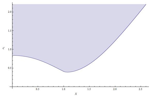
Figure 2: Plot of Good States: $EX(\infty)=1$

5 When Does Initial Transient Bias Matter?

Given the time-average estimator $\alpha(t)\stackrel{{\scriptstyle\Delta}}{{=}}t^{-1}\int_{0}^{t}f(X(s))ds$ for $\alpha=Ef(X(\infty))$, its (single replication) rate of convergence is determined by the central limit theorem (CLT). To develop the CLT for $\alpha(t)$, recall that $(M(t):\,t\geq 0)$ is a martingale; see Section 3. The martingale CLT as applied to the stochastic integral associated with the martingale then guarantees that

$$\sqrt{t}(\alpha(t)-\alpha)\Rightarrow\kappa N(0,\,1)$$

as $t\rightarrow\infty$, where $\kappa^{2}=\sigma^{2}Eh^{\prime}(X(\infty))^{2}$; see, for example, p.339-340 of Ethier and Kurtz (2005). The CLT asserts that the expected stochastic variability of $\alpha(t)$, for large $t$, is governed by $\kappa E|N(0,\,1)|t^{-1/2}=\kappa(2/\pi)^{1/2}t^{-1/2}$.

On the other hand, the systematic error in $\alpha(t)$ (namely, the bias) was analyzed in Section 3 and determined to be $\beta_{f}(\delta_{x})/t$ for $t$ large, assuming that the process was initialized at state $x$. It is clear that for $t$ large enough, the stochastic variability dominates the bias. Specifically, for $t\geq t^{*}(x)\stackrel{{\scriptstyle\Delta}}{{=}}\beta_{f}(\delta_{x})^{2}\pi/(2\kappa^{2})$, the bias contribution is smaller than the error due to stochastic variability.

To help put the quantity $t^{*}(x)$ in perspective, note that the CLT suggests that a relative error $\epsilon^{*}=2\kappa(2/\pi)^{1/2}/(t^{*}(x)^{1/2}|Ef(X(\infty))|)$ is achieved at a run-length $t^{*}(x)$ (contributed in equal measures from stochastic variability and bias). In other words,

$$\epsilon^{*}(x)\stackrel{{\scriptstyle\Delta}}{{=}}\frac{2\kappa^{2}}{|\beta_{f}(\delta_{x})|\cdot|Ef(X(\infty))|}\frac{2}{\pi}$$

is the relative precision at which a simulation designed to achieve such an error tolerance will have an error that is contributed equally from stochastic variability and initial transient bias. At all smaller values of the relative precision, the stochastic variability dominates the error. In particular, to achieve a relative error tolerance of $\epsilon=\nu\epsilon^{*}(x)$ (with $\nu<1$), the associated run-length $t$ that must be used is such that the error due to initial transient bias at such a run-length is roughly a proportion $\nu$ of the stochastic error. Thus, the quantity $\epsilon^{*}(x)$ is an important measure of the threshold error tolerance at which the initial transient is no longer a dominant source of error in computing steady-state quantities.

Figure 3 below provides a graph of the threshold error tolerance as a function of $x$ for $f(y)=y$, with $(r,\,\sigma^{2})=(1,\,2)$. Given that a relative error precision of $10\%$ or less is typically desired, we note that the set of states $x$ for which $\epsilon^{*}(x)\geq 0.1$ is large, specifically the interval $[0,\,10.19]$.

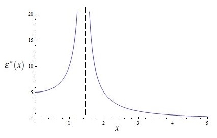
Figure 3: Plot of $\epsilon^{*}(x)$ vs. $x$: $r=1$ and $\sigma^{2}=2$

6 Mean Square Error for RBM Equilibrium Calculations

Because mean square error (MSE) is so frequently utilized in theoretical analyses of the initial transient problem, we provide here a detailed analysis of MSE in the setting of RBM. For a given performance measure $f$, recall the martingale $(M(t):\,t\geq 0)$ of Section 3. Hence, in view of the martingale property of the stochastic integral,

$$E_{x}\left(\int_{0}^{t}f_{c}(X(s))ds\right)^{2} = \sigma^{2}\int_{0}^{t}E_{x}h_{c}^{\prime}(X(s))^{2}ds+h_{c}^{2}(x)+E_{x}h_{c}^{2}(X(t))$$

$$\qquad- 2E_{x}h_{c}(x)h_{c}(X(t))-2\sigma E_{x}h_{c}(X(t))\int_{0}^{t}h_{c}^{\prime}(X(s))dB(s).$$

But

$$E_{x}h_{c}(X(t))\int_{0}^{t}h_{c}^{\prime}(X(s))dB(s) = E\left[h_{c}(X(0))\int_{-t}^{0}h_{c}^{\prime}(X(s))dB(s)\,\bigg{|}\,X(-t)=x\right]$$

$$= Eh_{c}(X^{*}(0))\int_{-\infty}^{0}h_{c}^{\prime}(X^{*}(s))dB(s)+o(1)$$

as $t\rightarrow\infty$, where $o(1)$ is a deterministic function tending to $0$ as $t\rightarrow\infty$, and $(X^{*},\,B)=((X^{*}(t),\,B(t)):\,-\infty<t<\infty)$ is such that $X^{*}$ is a stationary RBM driven by the Brownian motion $B$. Of course,

$$Eh_{c}(X^{*}(0))\int_{-\infty}^{0}h^{\prime}_{c}(X^{*}(s))dB(s)=-Eh_{c}(X^{*}(0))\int_{0}^{\infty}h_{c}^{\prime}(X^{*}(-s))dB(-s).$$ (6.1)

Since $X^{*}$ is a reversible one-dimensional diffusion driven by $B$ (see, for example, Kent (1978)),

$$((X^{*}(-t),\,-B(-t)):-\infty<t<\infty)\stackrel{{\scriptstyle\mathscr{D}}}{{=}}((X^{*}(t),\,B(t)):\,-\infty<t<\infty),$$

where $\stackrel{{\scriptstyle\mathscr{D}}}{{=}}$ denotes equality in distribution. Consequently, (6.1) equals

$$Eh_{c}(X^{*}(0))\int_{0}^{\infty}h_{c}^{\prime}(X^{*}(t))dB(t)=0,$$

because of the martingale property of the stochastic integral.

Furthermore, $E_{x}h_{c}^{2}(X(t))=Eh_{c}^{2}(X(\infty))+o(1)$ as $t\rightarrow\infty$ and $E_{x}h_{c}(X(t))=Eh_{c}(X(\infty))+o(1)$ as $t\rightarrow\infty$. Finally, by following the same argument as in Section 3, we find that

$$\int_{0}^{t}E_{x}h^{\prime}(X(s))^{2}ds = tEh^{\prime}(X(\infty))^{2}+\int_{0}^{t}(E_{x}h_{c}^{\prime}(X(s))^{2}-Eh_{c}^{\prime}(X(\infty))^{2})ds$$

$$= \kappa^{2}t/\sigma^{2}+k_{c}(x)+o(1)$$

as $t\rightarrow\infty$, where $k_{c}$ is the solution of the Poisson’s equation associated with $h_{c}^{\prime 2}$, namely $k_{c}$ satisfies

$$(\mathscr{L}k_{c})(x)=-(h_{c}^{\prime}(x)^{2}-Eh_{c}^{\prime}(X(\infty))^{2}),\;\;x\geq 0$$

subject to $k_{c}^{\prime}(0)=0,\;\;Ek_{c}(X(\infty))=0$. In view of (3.1),

$$k_{c}(x)=-\frac{1}{r}\int_{0}^{x}h_{c}^{\prime}(y)^{2}\left(e^{-\eta(y-x)}-1\right)dy+\frac{2}{\sigma^{2}}\int_{0}^{\infty}\int_{0}^{x}h_{c}^{\prime}(y)^{2}(e^{-\eta y}-e^{-\eta x})dydx.$$

With $k_{c}$ now computed, the mean square error of $\alpha(t)$ is given by

$$E(\alpha(t)-\alpha)^{2}=\frac{\kappa^{2}}{t}+\frac{\sigma^{2}k_{c}(x)}{t^{2}}+\frac{h_{c}(x)^{2}}{t^{2}}+\frac{Eh_{c}^{2}(X(\infty))}{t^{2}}+\frac{1}{t^{2}}o(1)$$ (6.2)

as $t\rightarrow\infty$. In particular, for $f(x)=x$,

$$E(\alpha(t)-\alpha)^{2} = \frac{\sigma^{6}}{2r^{4}t}+\frac{\sigma^{2}\left(2r^{3}x^{3}+3r^{2}\sigma^{2}x^{2}-3\sigma^{6}\right)}{6r^{6}t^{2}}+\frac{\left(\sigma^{4}-2r^{2}x^{2}\right)^{2}}{16r^{6}t^{2}}+\frac{5\sigma^{8}}{16r^{6}t^{2}}+\frac{1}{t^{2}}o(1)$$

$$= \frac{\sigma^{6}}{2r^{4}t}+\frac{6r^{4}x^{4}+8r^{3}\sigma^{2}x^{3}+6r^{2}\sigma^{4}x^{2}-3\sigma^{8}}{24r^{6}t^{2}}+\frac{1}{t^{2}}o(1)$$

as $t\rightarrow\infty$.

The term $h_{c}(x)^{2}/t^{2}$ is the squared bias contribution to the MSE due to the initial transient. The expression (6.2) makes clear that the MSE includes other state-dependent contributions of the same order of magnitude (that are contributed by the variance of $\alpha(t)$ rather than the bias), namely $\sigma^{2}k_{c}(x)/t^{2}$. Hence, a full analysis of the MSE impact of the effect of the initial transient should also (ideally) include an analysis of this variance term involving $k_{c}$, in addition to the bias contribution that is typically included in such an MSE analysis.

7 Conclusion

We have developed various formulae related to the initial transient problem for RBM. These formulae can be used directly in a simulation context, to approximate the impact of the initial transient for queueing simulations for which RBM is a suitable guide (eg. simulations of queues in heavy traffic). Our formulae also make clear a key insight that is likely true in a much broader class of simulations. In particular, for RBM, there is typically a robust set of initializing states for which the impact of the initial transient is roughly comparable to that associated with initializing in equilibrium. Since initializing in equilibrium corresponds to a setting in which there is no initial transient, this suggests that one should not worry excessively about the initial transient unless one has inadvertently initialized the simulation with a very poor (“bad”) choice of state. If one instead initializes with a reasonable (“good”) choice of state, the key element to a successful calculation of $Ef(X(\infty))$ is ensuring that the run-length is long enough to ensure that the stochastic variability has been reduced to a level commensurate with the desired accuracy. This suggests that a focus of initial transient research should be on building reliable algorithms for identifying settings in which one has inadvertently chosen a poor initialization that induces a large transient.

8 Acknowledgements

We thank the referees for their helpful comments and suggestions. Rob J. Wang is grateful to be supported by an Arvanitidis Stanford Graduate Fellowship in Memory of William K. Linvill, as well as an NSERC Postgraduate Scholarship (PGS D).

9 Author Biographies

ROB J. WANG is currently a Ph.D. candidate in Management Science and Engineering at Stanford University, specializing in Operations Research. He holds a B.Sc. (Honours) in Mathematics from Queen’s University in Kingston, Ontario (Canada). His research interests include simulation output analysis, queueing theory, diffusion processes, and statistical inference. His email address is robjwang@stanford.edu and his webpage is http://web.stanford.edu/$\sim$robjwang/.

PETER W. GLYNN is currently the Chair of the Department of Management Science and Engineering and Thomas Ford Professor of Engineering at Stanford University. He is a Fellow of INFORMS and of the Institute of Mathematical Statistics, has been co-winner of Best Publication Awards from the INFORMS Simulation Society in 1993 and 2008, and was the co-winner of the John von Neumann Theory Prize from INFORMS in 2010. In 2012, he was elected to the National Academy of Engineering. His research interests lie in stochastic simulation, queueing theory, and statistical inference for stochastic processes. His email address is glynn@stanford.edu and his webpage is http://web.stanford.edu/$\sim$glynn/.

References

- Ethier and Kurtz (2005) S. N. Ethier and T. G. Kurtz. Markov Processes: Characterization and Convergence. John Wiley & Sons, New York, second edition, 2005.
- Grassmann (2011) Winfried K. Grassmann. Rethinking the initialization bias problem in steady-state discrete event simulation. In S. Jain, R. R. Creasey, J. Himmelspach, K. P. White, and M. Fu, editors, Proceedings of the 2011 Winter Simulation Conference, pages 593–599, 2011.
- Grassmann (2014) Winfried K. Grassmann. Factors affecting warm-up periods in discrete event simulation. Simulation, 90(1):11–23, 2014.
- Harrison (1985) J. M. Harrison. Brownian Motion and Stochastic Flow Systems. John Wiley & Sons, New York, 1985.
- Iglehart and Whitt (1970) Donald L. Iglehart and Ward Whitt. Multiple channel queues in heavy traffic. I. Adv. Appl. Probab., 2(1):150–177, 1970.
- Karlin and Taylor (1981) S. Karlin and H. M. Taylor. A Second Course in Stochastic Processes. Academic Press, New York, 1981.
- Kent (1978) John Kent. Time-reversible diffusions. Adv. Appl. Probab., 10:819–835, 1978.
- Linetsky (2005) Vadim Linetsky. On the transition densities for reflected diffusions. Adv. Appl. Prob., 37:435–460, 2005.
- Pollard (2002) David Pollard. A User’s Guide to Measure Theoretic Probability. Cambridge University Press, Cambridge, 2002.
- Wang and Glynn (2014) Rob J. Wang and Peter W. Glynn. On the marginal standard error rule and the testing of initial transient deletion methods. Submitted, pages 1–27, 2014.