Molecular gas heating in Arp 299 ^,

(Ultra) luminous infrared galaxies ((U)LIRGs) are nearby laboratories that allow us to study similar processes to those occurring in high redshift submillimeter galaxies. Understanding the heating and cooling mechanisms in these galaxies can give us insight into the driving mechanisms in their more distant counterparts. Molecular emission lines play a crucial role in cooling excited gas, and recently, with Herschel Space Observatory we have been able to observe the rich molecular spectrum. Carbon monoxide (CO) is the most abundant and one of the brightest molecules in the Herschel wavelength range. CO transitions from J=4-3 to 13-12 are observed with Herschel, and together, these lines trace the excitation of CO. We study Arp 299, a colliding galaxy group, with one component (A) harboring an AGN and two more (B and C) undergoing intense star formation. For Arp 299 A, we present PACS spectrometer observations of high-J CO lines up to J=20-19 and JCMT observations of ¹³CO and HCN to discern between UV heating and alternative heating mechanisms. There is an immediately noticeable difference in the spectra of Arp 299 A and Arp 299 B+C, with source A having brighter high-J CO transitions. This is reflected in their respective spectral energy line distributions. We find that photon-dominated regions (PDRs, UV heating) are unlikely to heat all the gas since a very extreme PDR is necessary to fit the high-J CO lines. In addition, this extreme PDR does not fit the HCN observations, and the dust spectral energy distribution shows that there is not enough hot dust to match the amount expected from such an extreme PDR. Therefore, we determine that the high-J CO and HCN transitions are heated by an additional mechanism, namely cosmic ray heating, mechanical heating, or X-ray heating. We find that mechanical heating, in combination with UV heating, is the only mechanism that fits all molecular transitions. We also constrain the molecular gas mass of Arp 299 A to $3\times 10^{9}$ M_⊙ and find that we need 4% of the total heating to be mechanical heating, with the rest UV heating. Finally, we caution against the use of ¹²CO alone as a probe of physical properties in the interstellar medium.

1 Introduction

(Ultra) luminous infrared galaxies ((U)LIRGs) are systems or galaxies with very high far-infrared luminosity (ULIRG: L${}_{FIR}>10^{12}L_{\odot}$ and LIRG: L${}_{FIR}>10^{11}L_{\odot}$; Sanders & Mirabel (1996)) owing to a period of intense star formation. Arp 299 (NGC 3690 + IC 694, Mrk 171, VV 118, IRAS 11257+5850, UGC6471/2) is a nearby (42 Mpc Sargent & Scoville (1991)) LIRG (L${}_{FIR}=5\times 10^{11}$) currently undergoing a major merger event. Arp 299 is dominated by intense, merger-induced star formation and is made up of three main components (Alonso-Herrero et al. 2000). Although the core regions of these components can still be resolved, there is a large overlap in their disks. The separation between Arp 299 A and Arp 299 B and C is 22”, or 4.5 kpc in physical distance. Arp 299 B and C are separated by only 6.4”, or 1.4 kpc. The largest component is the massive galaxy IC 694 (Arp 299 A), which accounts for about 50% of the galaxies’ total infrared luminosity (Alonso-Herrero et al. 2000).

The galaxy NGC 3690 represents the second component (Arp 299 B) that is merging into IC 694 and represents $\sim 27\%$ of the total luminosity (Alonso-Herrero et al. 2000). The third component (Arp 299 C) is an extended region of star formation where the two galaxy disks overlap. Here we use the standard nomenclature, instead of the NED definition. Sargent & Scoville (1991) suggest that an active galactic nucleus (AGN) could be responsible for the large amount of far-infrared luminosity in Arp 299 A, although Alonso-Herrero et al. (2000) find no supporting evidence. Henkel et al. (2005) and Tarchi et al. (2007) suggest that the presence of H₂O masers, along with X-ray imaging and spectroscopy (Della Ceca et al. 2002; Zezas et al. 2003; Ballo et al. 2004) indicate that an AGN must be present in the nuclear region of Arp 299 A. Using milliarcsecond 5.0 GHz resolution images from the VLBI, Pérez-Torres et al. (2010) conclude that there is a low luminosity AGN (LLAGN) at the center of Arp 299 A.

In addition to the AGN, there are intense knots of star formation observes in the infrared and radio (Wynn-Williams et al. 1991). Alonso-Herrero et al. (2000) observes Arp 299 in high-resolution with the Hubble Space Telescope in the near-infrared and also find that over the past 15 Myr, Arp 299 has been undergoing intense merger-related star formation. This star formation is fueled by large amounts of dense molecular gas: 8$\times 10^{5}$ M_⊙ pc^-2 for Arp 299 A, 3$\times 10^{4}$ M_⊙ pc^-2 for Arp 299 B, and 2$\times 10^{4}$ M_⊙ pc^-2 for Arp 299 C (Sargent & Scoville 1991). Most of the star formation responsible for the high far-infrared luminosity is spread over 6-8 kpc (Alonso-Herrero et al. 2009), resulting in most of Arp 299 having typical starburst properties. Only the nucleus of Arp 299 A exhibits true LIRG conditions, with n_e=1-5$\times 10^{3}$ cm^-3, deep silicate absorption features implying embedded star formation, and PAH emission (Alonso-Herrero et al. 2009).

In this paper we present observations of the central region of Arp 299 using the Spectral and Photometric Imaging Receiver (SPIRE) on board of the ESA Herschel Space Observatory as part of HerCULES (PI: P. P. van der Werf). Due to the large spectral range of SPIRE, we can observe many different line transitions, which enables the study of excitation mechanisms of different phases of the ISM. Specifically, we compare the intensity of different CO transitions to CO emission models to determine the density, temperature, and radiation environment of the phases of the ISM in Arp 299. We directly compare Arp 299 A, which harbors an AGN, to Arp 299 B and C, which are undergoing rapid star formation. Then we add observations from the Photodetector Array Camera and Spectrometer (PACS) (PI: R. Meijerink) and the literature to disentangle the heating mechanisms of the molecular gas. In Section 2 we present all of the observations and discuss the data reduction methods. Then in Section 3, we present the spectra and line fluxes for both the SPIRE and PACS spectra. A qualitative comparison between Arp 299 A, B, and C is discussed in Section 4. Using all available data, in Section 5 we explore the heating mechanisms of the highest-J CO transitions and discuss the limitations of using only ¹² CO to determine physical parameters in Section 6. We state our conclusions in Section 7.

2 Observations and data reduction

2.1 Observations

Table 1: Log of Herschel Observations

Instru-	Transition	Observation ID	Date	Integr.
ment			Y-M-D	[s]
Arp 299 A $11^{h}28^{m}33^{s}.7$ $+58^{d}33^{m}46^{s}$
PACS	CO $J=14-13$	1342232607	2011-11-21	4759
PACS	CO $J=16-15$	1342232606	2011-11-21	641
PACS	CO $J=18-17$	1342232608	2011-11-22	782
PACS	CO $J=20-19$	1342232603	2011-11-21	1225
PACS	CO $J=22-21$	1342232605	2011-11-21	976
PACS	CO $J=24-23$	1342232603	2011-11-21	1225
PACS	CO $J=28-27$	1342232607	2011-11-21	4759
SPIRE	$194-671$ $\mu$m	1342199248	2011-06-27	4964
Arp 299 B $11^{h}28^{m}31^{s}$ $+58^{d}33^{m}41^{s}$
SPIRE	$194-671$ $\mu$m	1342199249	2011-06-27	4964
Arp 299 C $11^{h}28^{m}31^{s}.13$ $+58^{d}33^{m}48^{s}.2$
SPIRE	$194-671$ $\mu$m	1342199250	2011-06-27	4964

Herschel SPIRE FTS data: Observations of Arp 299 were taken with the Herschel Spectral and Photometric Imaging Receiver and Fourier-Transform Spectrometer (SPIRE-FTS, Griffin et al. 2010) on board the Herschel Space Observatory (Pilbratt et al. 2010) using three separate pointings centered on Arp 299 A, Arp 299 B, and Arp 299 C (see Table 1). The low frequency band covers $\nu$=447-989 GHz ($\lambda$=671-303 $\mu$m) and the high frequency band covers $\nu$=958-1545 GHz ($\lambda$=313-194 $\mu$m), and these bands include the CO J=4-3 to CO J=13-12 lines. The high spectral resolution mode was used with a resolution of 1.2 GHz over both observing bands. Each source was observed for 4964 seconds (1.4 hours). A reference measurement was used to subtract the emission from the sky, telescope, and instrument. We present the original observed SPIRE spectra in Figure 1.

Herschel SPIRE Photometry data: Observations using the SPIRE Photometer were taken as part of the Herschel Guaranteed Time Key Program SHINING (PI: E. Sturm). The system was observed on the 6th of January 2010 at 250, 350, and 500 $\mu$m (observation ID: 1342199344, 1342199345, 1342199346). The source was observed 797 seconds in total.

Herschel PACS spectroscopy data: CO $J_{up}\geq 14$ observations were made with the Photodetector Array Camera and Spectrometer (PACS, Poglitsch et al. 2010) for Arp 299 A only. The data presented here have been obtained as part of the Herschel program OT1_rmeijeri_1 (PI: Meijerink), complemented by observations from OT1_shaileyd_1 (PI: Hailey-Dunsheath). The observations consisted of deep integrations targeting CO $J=14-13$, CO $J=16-15$, CO $J=18-17$, CO $J=20-19$, CO $J=22-21$, CO $J=24-23$, and CO $J=28-27$. The observation IDs of the targeted CO lines are listed in Table 1.

Ground based data: We use the short spacing corrected CO maps from Sliwa et al. (2012) for the J=1-0, 2-1, and 3-2 transitions for Arp 299 B and C. We integrate the flux corresponding to our largest SPIRE beam (J=4-3, 42”) full-width-half-maximum (FWHM) centered on each of the pointings respectively. We do not use these values for Arp 299 A since the CO 1-0 map has error bars larger than 50%.

For Arp 299 A, we used dual-polarisation receivers A and B (decommissioned in 2009) on the IRAM 30 m telescope to measure the $J$=1-0 ¹²CO line towards Arp 299 in November 2005, followed by observations of $J=2-1$ ¹²CO and both $J$=1-0 and $J$=2-1 ¹³CO in July 2006. Weather conditions were good to excellent. System temperatures including the sky were 160 K to 240 K for the $J$=1-0 transitions and 400 - 500 K for the $J$=2-1 transitions. Beam sizes are $21"$-$22"$ and 11” at 110-115 GHz and 220-230 GHz corresponding to these transitions. Main-beam efficiencies were 0.74, 0.73, 0.48, and 0.45 at these four frequencies, respectively. The $J$=2-1 ¹²CO and ¹³CO lines were also observed with the JCMT 15 m telescope in June and July 1995, with overall system temperatures including the sky of 485 and 340 K, respectively. The beam size was $21"-22"$, and the main-beam efficiency was 0.69. All spectra were binned to resolutions of 20 km/s. A linear baseline was subtracted, and the line flux was determined by integrating over the velocity range V(LSR) = 2800 - 3500 km/s.

The HCN J=(3-2) observations were made with the JCMT in February 2010 using receiver A3 under good weather conditions with system temperatures of 240 to 310 K; the beam size was $18"$, and we used a main-beam efficiency of 0.69 at the operating frequency of 265.9 GHz. HCN J=(4-3) was obtained with the HARP array in stare mode on the JCMT in May 2010. Weather was excellent, with T(sys) in the range of 226-240 K. We extracted the line profile from the central pixel. The beam size was about $13"$ and the main-beam efficiency about 0.6. From the observed spectra, line fluxes were recovered in the same way as for the ¹³CO observations.

2.2 Data reduction

Herschel SPIRE FTS data: The data were reduced using version 9.0 of Herschel Interactive Processing Environment (HIPE). For all extended sources, an aperture correction is necessary to compensate for the wavelength dependent beam size. This requires knowledge of the source distribution at SPIRE wavelength. We approximated the size based on a high spatial resolution SMA CO J=3-2 map (Wilson et al. 2008).

Each SMA map was convolved with a 2-D Gaussian to match the FWHM of the SPIRE beam sizes (15-42”). We then determine the flux density at the SPIRE pointing centers as a function of spatial resolution normalized by the flux density in the largest aperture (42”). The resulting dependency between normalized flux density and spatial resolution was then applied to SPIRE’s Long Wavelength Spectrometer Array (SLW) and the Short Wavelength Spectrometer Array (SSW) spectra taking the SPIRE beam sizes as a function of wavelength into account. Finally the SLW and SSW spectra were coadded flagging the noisy edge channels in both spectra. This yields a combined spectrum at an effective spatial resolution of 42” for each source.

The quality of the aperture correction can easily be evaluated by comparing the continuum flux densities in the corrected SLW and SSW spectra in their spectral overlap region. Our approach effectively removes the ’jump’ visible in the continua between the SLW and SSW spectra at their original spatial resolution, although we only present the original observed spectra below.

The ratio of the flux between each convolved SMA map and the flux within the largest beam size (42”) is the beam correction factor ($\kappa_{S}$) where:

$$F_{corr}=F_{obs}\times\kappa_{S}$$ (1)

Thus, all fluxes are normalized to a beam size of 42” (i.e. 9.8 kpc). The beams for pointings B and C significantly overlap, thus it is hard to discern any independent measurements from these pointings. However, pointing A is more isolated. Although the largest beam does include some of B and C, most of the beam sizes are completely independent.

Fluxes were first extracted using FTFitter (https://www.uleth.ca/phy/naylor/index.php?page=ftfitter), a program specifically created to extract line fluxes from Fourier transform spectrographs. This is an interactive data language (IDL) based graphical user interface that allows the user to fit lines, choose line profiles, fix any line parameter, and extract the flux. We define a polynomial baseline to fit the continuum and derive the flux from the baseline subtracted spectrum. In order to more accurately determine the amplitude of the line, we fix the FWHM to the expected line width of ¹²CO at each source, using the velocity widths measured by Sliwa et al. (2012). In the case of very narrow linewidths, more narrow than the instrumental resolution (J= 4-3 through 8-7 for Arp 299 C), we do not fix the FWHM but fit the lines as an unresolved profile. We use an error of 30% for our fluxes, which encompasses our dominant sources of error. Specifically, the uncertainty of the beam size correction using SMA CO J=3-2 map is $\sim$20%. The error of the absolute calibration uncertainty for staring-mode SPIRE FTS observations is an additional 6% (Swinyard et al. 2014). We also have some uncertainty in the definition of the baseline and flux extractions, since we use an unresolved or Gaussian profile for all emission lines, accumulating to $\sim 5\%$.

Herschel SPIRE photometry data: SPIRE maps were reduced using HIPE 10.3.0 (Ott 2010) and the SPIRE calibration tree v.10.1. A baseline algorithm (Bendo et al. 2010) was applied to every scan of the maps in order to correct for offsets between the detector timelines and remove residual baseline signals. Finally, the maps were created using a naive mapping projection. The global fluxes for Arp 299 are measured to be 21.8, 7.34 and 2.37 Jy for 250, 350 and 500 $\mu$m respectively. For the errors in the SPIRE photometry we adopted a 15% calibration uncertainty for extended emission; (SPIRE Observers Manual, v2.4, 2011).

Herschel PACS data: The data were processed and calibrated using HIPE version 10.0 and the pipeline for range spectroscopy. The object was centered on the 9.4″central spaxel of the 5 by 5 PACS array. Little flux is seen outside this central spaxel, and therefore the fluxes are extracted from the central spaxel and referenced to a point source. We use a 3 by 3 spaxel correction for extended sources and small pointing offsets. We used SPLAT as part of the STARLINK software package to subtract baseline, and determine the peak flux, full-width-half maximum (FHWMs), integrated flux, and its uncertainty for the CO lines. To find the integrated flux and uncertainty, we fit a Gaussian profile to the line and integrate the Gaussian.

Ground Based Data: In the reduction of the line profiles observed with IRAM and JCMT, we used the CLASS package. The JCMT data were retrieved with the SpecX package and turned into FITS files which were subsequently imported into CLASS. The IRAM profiles were immediately available in CLASS format. For all line profiles, second-order baselines were subtracted. Line fluxes were determined both by Gaussian fitting, and by straightforward summing over a sufficiently wide velocity interval. Both methods yielded nearly identical results. We then scaled the ¹³CO J=1-0 and J=2-1 up to the 42” beamsize using the same method described in Section 2.2 for the SPIRE FTS observations.

3 Results

Here we present the spectral profiles and line fluxes for the SPIRE FTS spectra and the PACS observations.

3.1 SPIRE FTS line fluxes

The ¹²CO transitions are visible from J=4-3 to J=13-12. There were also strong detections of [NII] at 1437 GHz and [CI] at 484 GHz and 796 GHz in all three spectra. We detect 7 strong water emission lines, they are most prominent in Source A and become weaker or undetectable in Sources B and C. The lines are labeled in Figure 1, ¹²CO in black, H₂O in blue, and atomic lines in magenta. As seen in this plot there is a discontinuity between the high and low frequency modes of the spectrometer. This discontinuity is due to the different apertures used by the high and low frequency arrays combined with the fact that the object is not a point source. A scaling factor ($\kappa_{S}$) for each wavelength is calculated using the method described in Section 2.2, and displayed in Table 1.

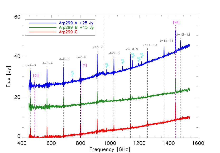
Figure 1: SPIRE spectra of Arp 299 A (blue), B (green) and C (red). Source A is offset by 25 Jy, while Source B is offset by 15 Jy. Each bright line is identified, CO lines in black, atomic lines in magenta, and H₂O lines in cyan. The atomic lines and H₂O transitions will be discussed in a different paper.

Table 2: Observed line fluxes corrected for beam size using correction factors ($\kappa_{S}$, Section 2.2). Also, the errors on all derived fluxes are 30% as explained in the text. Fluxes from ground-based observations found in the literature are also presented.

Line	$\kappa_{S_{A}}$	Flux Arp 299 A	$\kappa_{S_{B}}$	Flux Arp 299 B	$\kappa_{S_{C}}$	Flux Arp 299 C
	32.8”	[10-17 W m-2]	32.8”	[10-17 W m-2]	32.8”	[10-17 W m-2]
12CO 4-3	1.01	8.89	1.02	5.28	1.02	5.88
12CO 5-4	1.10	10.8	1.26	6.75	1.24	7.45
12CO 6-5	1.14	12.5	1.40	7.18	1.38	7.02
12CO 7-6	1.07	13.0	1.19	6.39	1.18	6.29
12CO 8-7	1.05	14.2	1.12	6.82	1.12	7.31
12CO 9-8	1.30	13.4	1.39	3.86	1.30	3.97
12CO 10-9	1.33	14.5	1.51	4.80	1.45	3.65
12CO 11-10	1.33	13.2	1.53	3.84	1.47	3.37
12CO 12-11	1.34	11.4	1.57	2.72	1.53	2.29
12CO 13-12	1.35	10.9	1.59	3.45	1.55	1.66
$[CI]^{3}P_{1}-^{3}P_{0}$	1.04	2.56	1.09	2.17	1.08	1.94
$[CI]^{3}P_{2}-^{3}P_{1}$	1.07	8.46	1.19	4.61	1.18	4.49
$[NII]^{3}P_{1}-^{3}P_{0}$	1.35	25.6	1.59	11.1	1.55	5.86
12CO 1-0	–	0.29	–	0.08	–	0.01
12CO 2-1	–	1.29	–	0.76	–	0.73
12CO 3-2	–	5.09	–	2.10	–	3.04
13CO 1-0	–	0.01	–	–	–	–
13CO 2-1	–	0.15	–	–	–	–
HCN 1-0	–	0.003	–	–	–	–
HCN 3-2	2.52	0.04	–	–	–	–
HCN 4-3	3.77	0.03	–	–	–	–

3.2 PACS line fluxes

The PACS CO $J=14-13$, $16-15$, $18-17$, and $20-19$ line detections are shown in Fig. 2 and their peak flux, FWHM, and integrated fluxes are listed in Table 3. We also would like to note that the CO $J=20-19$ transition is only detected at 2$\sigma$. The CO $J=22-21$, $J=24-23$ and $28-27$ were not detected, and for these lines we determined an upper limit.

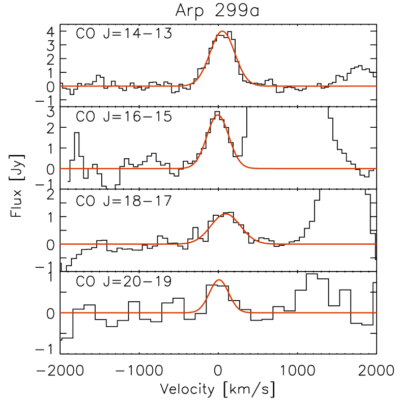
Figure 2: PACS spectra of Arp 299 A, showing the detections for CO J $=14-13$, $16-15$, $18-17$, and $20-19$. The J$=20-19$ transition is only a 2$\sigma$ detection. The line to the right of the J=$16-15$ transition, around 1000 km/s is the OH doublet ($\Pi_{1/2}-\Pi_{1/2}$ 3/2-1/2 163.124-163.397 $\mu$m), and the line to the right of the J=18-17 transition is the [OI] 145$\mu$m line. The velocity scale is calculated for a redshift of $z=0.01030$ and the channel spacings are 47, 57, 64, and 140 km/s for the J $=14-13$, $16-15$, $18-17$, and $20-19$ respectively.

Table 3: PACS CO observations.

Transition	$\lambda_{\rm rest}$	Peak	$\Delta V_{c}$	FWHM	$S_{\rm line}$	$S_{\rm line,corr}$
	[$\mu$m]	[Jy]	[km/s]	[km/s]	[10-17 W m-2]	[10-17 W m-2]
Arp 299 A
CO $J=14-13$	185.999	$4.0\pm 0.2$	$50\pm 7$	$367\pm 17$	$8.3\pm 0.5$	$11.2\pm 0.7$
CO $J=16-15$	162.812	$2.6\pm 0.1$	$-7\pm 6$	$326\pm 16$	$5.6\pm 0.3$	$7.5\pm 0.5$
CO $J=18-17$	144.784	$1.1\pm 0.1$	$92\pm 21$	$438\pm 50$	$3.6\pm 0.5$	$4.8\pm 0.7$
CO $J=20-19$	130.369	$0.8\pm 0.2$	$8\pm 36$	$285\pm 87$	$1.8\pm 0.7$	$2.4\pm 0.9$
CO $J=22-21$	118.581				$<2.3$	$<3.1$
CO $J=24-23$	108.763				$<2.6$	$<3.5$
CO $J=28-27$	93.3491				$<1.7$	$<2.3$

4 Comparison between Arp 299 A and B+C

In this section, we perform a comparison of Arp 299 A, B, and C using only the SPIRE FTS fluxes to determine what differences are observed from ¹²CO alone. The most notable aspect of the spectra presented in Figure 1 is that the high-J CO lines of Arp 299 A are distinctly brighter than those of Arp 299 B and C. It is clear simply from inspecting the spectra that the molecular gas in Arp 299 A is more excited than that of Arp 299 B and C.

For each spectrum (A, B, and C) we can create a spectral line energy distribution or ’CO ladder’, which plots the intensity of each CO transition as a function of the upper J number. This type of diagram is predicted to be a powerful diagnostic tool as shown by Meijerink & Spaans (2005) and Meijerink et al. (2007), where models show that these CO ladders have very different shapes depending on the type of excitation (i.e. photon dominated region, PDR or X-ray dominated region, XDR) as well as density and radiation environment. The three CO ladders for Source A, B, and C are plotted on top of each other in Figure 3. For context, their smallest and largest beam sizes are plotted over a SCUBA 450 $\mu$m image, showing the overlap between the Arp 299 B and C pointings. This overlap is also apparent in the CO ladders, the two ladders follow the same shape and intensity, meaning they are essentially an averaged observation of both Arp 299 B and C. Because of this, we only use the averaged values for Arp 299 B and C from here on. Although we cannot discern anything independent about Arp 299 B and C, it is immediately apparent that Arp 299 A has a very differnt CO ladder. Arp 299 A flattens in intensity with increasing transitions, while Arp 299 B and C both show a turnover in their ladders at J_upp=5. This indicates clearly that there is more warm CO in Arp 299 A than in B+C and we expect to see this reflected in the following PDR analysis.

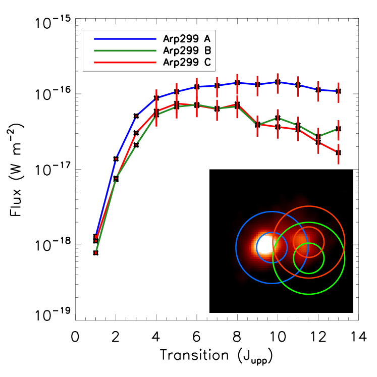
Figure 3: CO excitation ladders of Arp 299 A (blue), B (green), and C (red). Intensities are in W m^-2. The inset in the bottom right corner shows the three SPIRE beam FWHMs for Arp 299 A, B, and C overplotted on a SCUBA 450 $\mu$m archival image. The smaller circle represents the smallest beam FWHM ($\sim$17”) and the larger circle represents the largest beam FWHM ($\sim$42”).

4.1 Basic PDR analysis

Since Arp 299 is a LIRG with a high star formation rate, there must be a high density of OB stars and thus a high UV energy density. Through photoelectric heating and FUV pumping of H₂, the FUV photons heat the outer layers (A_V¡5) of molecular clouds. This area of the molecular cloud is the PDR, and is responsible for warm molecular gas emission. The thermal state of PDRs is determined by processes such as photo-electric heating; heating by pumping of H₂ followed by collisional de-excitation; heating by cosmic rays; [OI] and [CII] fine-structure line cooling; and CO, H₂O, H₂, and OH molecular cooling. The ionization degree of the gas is driven by FUV photo-ionization, and counteracted by recombination and charge transfer reactions with metals and PAHs. The ionization degree is at most $x_{\rm e}\sim 10^{-4}$ outside of the fully ionized zone. The chemistry exhibits two fundamental transitions, H to H₂ and C⁺ to C to CO. Using PDR models (Meijerink & Spaans 2005; Kazandjian et al. 2012) that solve for chemistry and thermal balance throughout the layers of the PDR, we use the predictions of the ¹²CO emission as a function of density, radiation environment ($G$, in units of the Habing radiation field G₀=1.6$\times 10^{-3}$ erg cm^-2 s^-1), and column density. We use an isotopic abundance ratio of 80 for ¹²CO/¹³CO, since our observed ¹²CO/¹³CO J=1-0 intensity ratio is $\sim 24$, which is common in (U)LIRGs (Aalto et al. 1997). González-Alfonso et al. (2012) find an isotope ratio around 100 for the prominent starburst Arp 220, which is similar to that of Mrk 231 (Henkel et al. 2014). However, for a less powerful starburst, such as NGC 253, the isotope ratio was measured to be 40 (Henkel et al. 2014). Since Arp 299 is a moderate starburst, an estimate of 80 is reasonable. The density profile is constant and the Habing field is parameterized in units of G₀ from photons between 6 eV and 13.6 eV. We perform an unbiased fitting of the models to the CO ladder, employing an automated $\chi^{2}$ fitting routine, described in detail in Rosenberg et al. (2014). This routine allows for up to 3 different ISM phases where we define the total model as:

$$Model=\Omega_{I}PDR_{I}+\Omega_{II}PDR_{II}+\Omega_{III}PDR_{III}$$ (2)

where $PDR_{I}$, $PDR_{II}$, and $PDR_{III}$ are the distinct contributions of the three PDR models. $\Omega_{I}$, $\Omega_{II}$, and $\Omega_{III}$ represent the respective filling factors of each ISM phase. Filling factors traditionally represent how much of the beam is filled, so they only range from 0 to 1. However, this assumes that these clouds do not overlap in velocity, which we allow for. Thus, $\Omega$ is not only a beam filling factor, but also allows for an overlap in velocity, which accounts for it being slightly greater than one.

We perform a modified Pearson’s $\chi^{2}$ minimized fit for ¹²CO and ¹³CO simultaneously, where the modified Pearson’s $\chi^{2}$ is:

$$\chi^{2}_{mol}=\frac{\sum_{i=1}^{N_{data}}\frac{(obs_{i}-model_{i})^{2}}{model_{i}}}{N_{data}}$$ (3)

We define $\chi^{2}_{mol}$ as the modified Pearson’s $\chi^{2}$ for a specific molecule. The total $\chi^{2}$ is the sum of the $\chi^{2}_{mol}$ terms for each molecule. The numerator of this equation is the traditional Pearson’s $\chi^{2}$, then in the denominator we divide by the total number of transitions in each respective molecule, essentially yielding an average $\chi^{2}$ for ¹²CO and ¹³CO separately. In Section 5, we refer to the total $\chi^{2}$ as being the sum of Eq. 3 for all molecules; ¹²CO, ¹³CO, and HCN.

Using this equation, we calculate the $\chi^{2}$ for every combination of 3 models and filling factors. In this way, we cannot only see which models make the best fit, but we can also see the $\chi^{2}$ values for all the other model combinations. This allows us to understand the level of degeneracy inherent to the models and understand the limitations of this method. In Figure 4, we show the best fitting models for Arp 299 A and Arp 299 B+C. We also calculate the relative contribution of each independent model to the overall CO ladder intensity in terms of emission and CO column density.

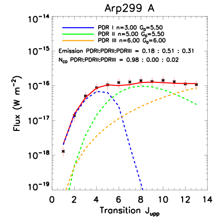
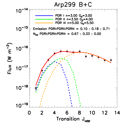
Figure 4: Best fit ($\chi^{2}$ minimized) PDR models simulating the ¹²CO emission for Arp 299 A (left)and B$+$C (right) using three ISM phases.

The red line is the sum of the three phase models, the black asterisks are the data points with error bars, and the blue, green, and orange lines represent the independent PDR models for each phases. The model density, temperature and column density are shown in the legend along with the relative contribution of each phase in terms of emission and column density.

One aspect of these fits is that each of the CO ladders needs a minimum of three ISM phases to be fit well. In addition, the lowest J transitions are fit with a relatively low density and low $G$ PDR, the middle phase is a medium density and medium $G$ PDR, and finally the highest J transitions can only be fit by extreme PDRs, which makes up a negligible percent of the CO column density, but over 30% of the total CO emission in the case of Arp 299 A and over 60% of the total CO emission in Apr299 B+C. In Figure 5, we display the degeneracy plots for Arp 299 B+C. These plots are only a slice of the full degeneracy cube, held at the best fit column densities. They are a representative example of the degeneracy plots of the other fits and share similar characteristics. In the left panel, we show the degeneracy plot for the first ISM phase (PDR I). Each small square represents a different model with a particular density and radiation. The color represents the $\chi^{2}$ value, white being the lowest and black being the highest.

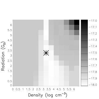
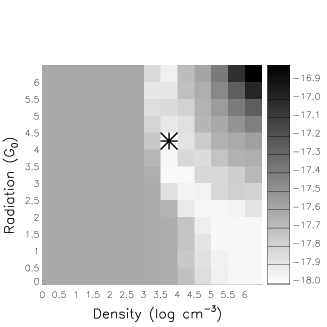
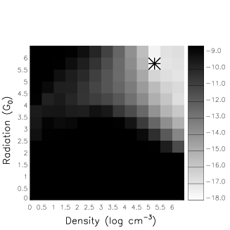
Figure 5: Degeneracy plots for Arp 299 B+C. Each plot represents the full grid of models for each phase in Figure 4, PDR I (left), PDR II (center), PDR III(right). The asterisk represents the model with the lowest $\chi^{2}$, which are also plotted in Figure  4. The gray scale of each small square indicates the associated log($\chi^{2}$) value for that particular model, white being the best fits and black being the worst. The $\chi^{2}$ value is defined in Equation 3 and shown in log gray scale.

As seen in Figure 5, the fits are degenerate. We do have a ’best fit’, designated with an asterisk, but especially in the case of PDR I, there are a wide range of models that would fit almost as well as the selected model. We can only constrain density to $n=10^{2.5}-10^{5.5}$ cm^-3 and the radiation field in unconstrained. Even though the fits are degenerate, it is clear that each phase has a specific and independent range of parameter space for which there is a good fit. Each ISM phase has a trade off between radiation and density, but each cover a different range of values. For instance, PDR I ranges in density from $n=10^{2.5}-10^{5.5}$ cm^-3, while PDR II ranges from $n=10^{3}-10^{6}$ cm^-3 and PDR III ranges from $n=10^{5.0}-10^{6}$ cm^-3. The radiation field strength is not as well constrained and varies inversely to the density. However without more information, we cannot break the observed degeneracies.

Since we have ancillary data for Arp 299 A, and since we cannot separate the contributions from Arp 299 B and C, the following discussion will focus on Arp 299 A.

5 A case study: Arp 299 A

Using the PACS high-J ¹²CO as well as the JCMT ¹³CO, and HCN observations, we determine if Arp 299 A can be heated purely through UV heating or if additional heating sources are necessary. We can use the PACS observations presented in Section 3.2 to extend the SPIRE CO ladder from J_upp=13 to J${}_{up}=20$. We then add the observations of ¹³CO J=1-0 and J=2-1 to constrain column density and observations of HCN J=1-0, J=3-2, and J=4-3 to constrain the high density components. In addition, we extract fluxes from the SPIRE Photometry maps and combine them with observations from the literature in order to perform an SED analysis of the dust to help further disentangle UV from other heating sources.

5.1 The low-excitation phase

Before we blindly fit the full grid of models to our observations, we can constrain the first ISM phase, responsible for the low-J CO lines. Since ¹³CO is optically thin, the ratio of ¹³CO to ¹²CO constrains the optical depth, and in turn the column density. We have observations of ¹³CO 1-0 and 2-1 from the JCMT, as presented in Section 2. We can assume that the ¹³CO 1-0 and 2-1 lines arise from the same ISM phase that is responsible for the first few transitions of ¹²CO, and can run the automated fitting routine on the low-J transitions alone. The best fit is displayed in Figure 6. Since often, most of the ¹²CO is in low rotational states, we can help constrain the mass of the whole system by finding the mass of the low-excitation ISM phase. In this phase, we find a mass of 2$\times 10^{9}$ M_⊙ (Eq. 4), which represents $\sim$66% of the total molecular gas mass.

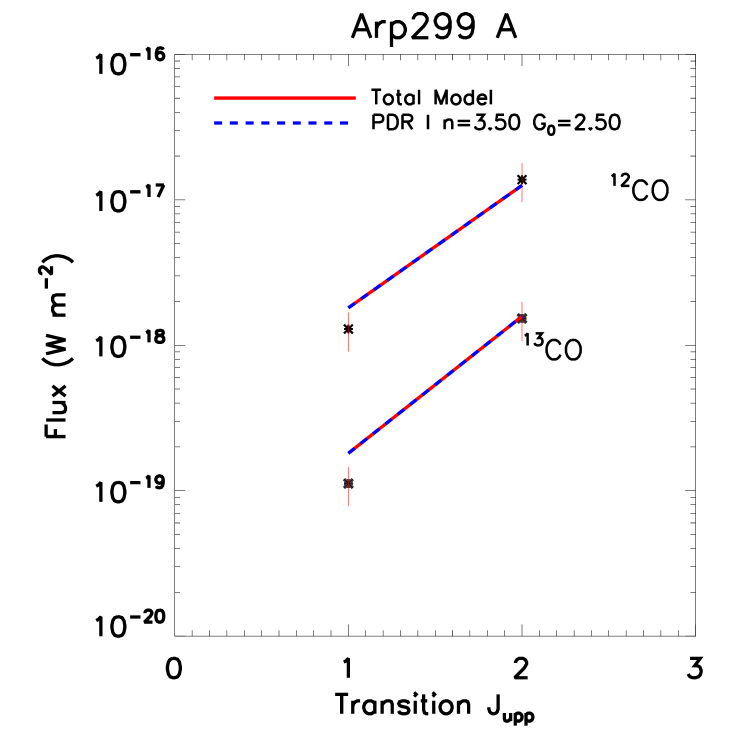
Figure 6: Best fit model of ¹³CO J¡2 and ¹²CO J¡2. The red line is the total model, the black asterisks are the data points with error bars, and the blue dotted line represents the first ISM phase, represented by a PDR model. The model density and radiation strength are shown in the legend.

5.2 Full PDR analysis

Now that we have constrained the first ISM phase, we can include all the available data to constrain the other ISM phases. We will include ¹²CO observations from PACS including J=14-13 through J=20-19 to constrain the CO ladder turn-over point, HCN 1-0, 3-2, and 4-3, to constrain the properties of the high density gas, and the SPIRE photometry observations to estimate the dust temperature. With all the available line fluxes, we can first fit the full CO and HCN ladders of Arp 299 A using pure PDR models. In Figure 7, we display the ¹²CO and ¹³CO ladders from J=1-0 through 28-27 and J=1-0 to 2-1 respectively, along with the $\chi^{2}$ minimized fits. We also calculate the relative contribution of each independent model to the overall CO ladder in terms of luminosity and CO column density.

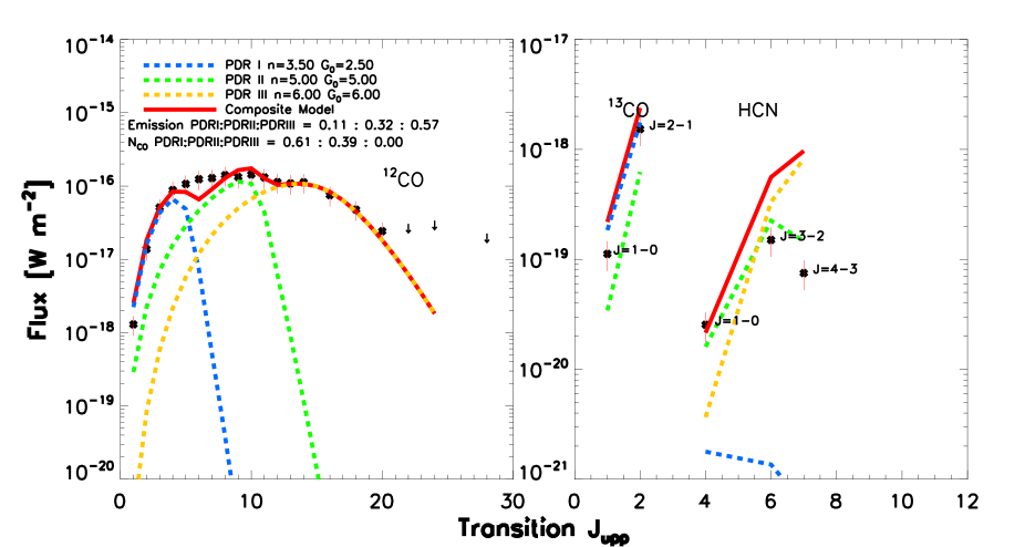
Figure 7: Left panel: A $\chi^{2}$ minimized fit of the CO ladder of Arp 299 A from J=1-0 through 24-23. The fit was constrained to three PDR models, displayed in blue, green, and yellow. The black points are the observed CO fluxes and the red line is the total model fit. Right panel: The same models as the left panel, but the fits for the ¹³CO and HCN fluxes. The HCN model lies far above the observed J=3-2 and 4-3 HCN fluxes.

The parameters of the fits are given in Table 3. We have estimated the masses of each ISM phase using the equation from Rosenberg et al. (2014):

$$M_{H_{2}}=\sum_{i}^{n}\frac{\Omega_{i}N_{H2,i}A_{beam}m_{H2}}{M_{\odot}}$$ (4)

where $N_{H2}$ is the H₂ column density in cm^-2 which is consistently calculated in the PDR models, $A_{beam}$ is the beam area in cmX ², and $m_{H2}$ is the mass of a hydrogen molecule.

We estimate the relative contributions of column density and emission to the total ¹²CO ladder. In order to estimate the relative contribution of emission, we use the following equation:

$$C_{em}=\rm\frac{\sum_{i=1}^{13}CO_{mod,i}}{CO_{tot}}$$ (5)

where ¹²CO_mod is the summed flux from the modeled CO transitions from J=1-0 to J=13-12 of a specific PDR model and ¹²CO_tot is the total model flux, defined in Eq. 2. We use the same method for calculating the contribution of column density, except we compare the column density of each PDR model to the total column density.

Table 4: Model parameters for the three molecular gas ISM phases using only PDR heating.

Component	Density log(nH)	log($G$)	log(NCO)	log(NH2)	$\Omega$	Cem	C${}_{N_{CO}}$	Mass${}_{N_{H2}}$
	log[cm-3]	G0	log[cm-2]	log[cm-2]				M⊙
Mtot: $2\times 10^{9}$ M⊙
PDR I	3.5	2.5	17.1	21.5	1.2	0.11	0.61	$2\times 10^{9}$
PDR II	5.0	5.0	18.2	21.9	0.06	0.32	0.39	$3\times 10^{8}$
PDR III	6.0	6.0	16.7	21.2	0.006	0.57	$<0.01$	$6\times 10^{6}$

Three pure PDR models fit the ¹²CO well, although the mid-J lines are not all fully reproduced. The ¹³CO is also very well reproduced. We find an H₂ mass of $3\times 10^{9}$ M_⊙, which matches the mass estimates from the literature, 1.8-8.6$\times 10^{9}$ M_⊙ (Sliwa et al. 2012; Sargent et al. 1987; Solomon & Sage 1988). As shown in Rosenberg et al. (2014), HCN is a good tracer of the excitation mechanism since the relative line ratios of various HCN transitions depend on excitation mechanism, and in the pure PDR fit, the models fail to fit any of the HCN transitions. Note that the red line for HCN lies far above the observed J=3-2 and 4-3 transitions. Since we cannot reproduce both the CO and HCN emission with the same best fit model, this suggests that there is an alternative heating mechanism responsible for heating the dense gas, which is traced by the HCN. In order to produce enough CO flux in the high-J transitions, the HCN is overproduced, thus we need a mechanism which selectively heats the high-J CO without heating as much HCN.

In addition, the only way to reproduce the flux of the high-J CO lines with a PDR is with a density of 10⁶ cm^-3 and a radiation flux of 10⁶ G₀, which is an order of magnitude higher than the most extreme PDRs (i.e. Orion Bar) found in the Milky Way. In terms of mass, this ISM phase represents about $\sim 0.2\%$ of the total molecular gas mass of Arp 299 A (Table 3). Since UV photons are even more efficient in heating the dust than the gas (unlike X-rays, cosmic rays, and mechanical heating), we expect the same percentage of the dust mass to be heated to high temperatures (¿200 K). Using a combination of three gray bodies, we can fit the SED with a ”cool”, ”warm”, and ”hot” dust component (see, e.g., Papadopoulos et al. (2010)) aiming to account for the cold cirrus-type dust, the star formation-heated dust, and an AGN-heated dust respectively. We caution the reader on the simplicity of the physics underlying this kind of modeling and especially for the emission at mid-infrared wavelengths where dust is primarily not in thermal equilibrium with the local interstellar radiation field. However this approach provides reasonable estimates for the average dust temperatures and masses for each component. The dust emissivity is a power law, where $\kappa_{\nu}=\kappa_{0}^{\beta}$. We assume a value of $\kappa_{0}$ = 0.192 m² kg^?1 at 350 $\mu m$ (Draine 2003) and $\beta$ = 2. The value $\beta$=2 was adopted as the most suitable for global dust emission SEDs (e.g.,Dunne & Eales (2001)). It has to be noted though that $\beta$ varies within galaxies (see, e.g., Tabatabaei et al. (2014)). To find the best fit SED our code minimizes the $\chi^{2}$ function using the Levenberg-Marquardt algorithm (Bevington & Robinson 1992). Besides the SPIRE data, which were reduced by us, we used the fluxes presented in U et al. (2012). The result of the three component fit is shown in Figure 7 (see the figure caption for an explanation of the symbols).

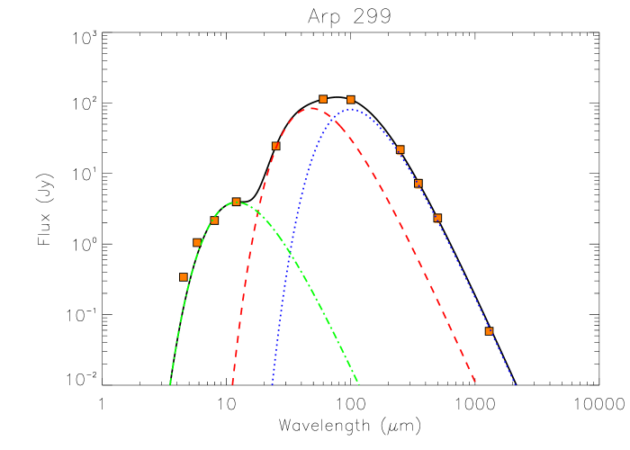
Figure 8: The dust SED of Arp 299. This is a fit with three gray bodies representing the cold (blue), warm (red) and hot (green) dust components. Observations are plotted with orange squares while the black line is the total SED model fit (Section 4.2).

The temperature and mass of each dust component is calculated. We find a temperature of 29.1$\pm 3.5$ K for the ”cool” component, 60.6$\pm 4.9$ K for the ”warm” component, and 239.4$\pm 22.7$ K for the ”hot” component. The dust masses are 1.1$\times 10^{8}$ M_⊙, 2.9$\times 10^{6}$ M_⊙, and 141 M_⊙, respectively. We find that the ”hot” dust component contains only $\sim 10^{-6}$ of the total dust mass. This is four orders of magnitude smaller than the 2$\times 10^{-2}$ of hot dust expected from a PDR with the parameters of PDR III (last column of Table 3). This along with the poor reproduction of HCN emission shows that the third ISM phase cannot be heated purely by UV photons.

5.3 Additional heating sources

We can explore alternative heating sources to explain the high-J CO and HCN transitions. We consider cosmic ray heating, X-ray heating, and mechanical heating (shocks and turbulence) as alternative heating sources. Cosmic rays can also heat gas in cosmic ray dominated regions (CDRs), which are PDRs with and enhanced cosmic ray ionization rate; we employ a typical model for enhanced cosmic ray ionization rate with $\zeta_{CDR}=750\zeta_{gal}$, 3.75$\times 10^{-14}$ s^-1. Cosmic rays are able to penetrate into the very centers of molecular clouds, where even X-rays have trouble reaching and are typically produced by supernovae. Similarly, PDRs with additional mechanical heating (mPDRs) are due to turbulence in the ISM and may be driven by supernovae, strong stellar winds, jets, or outflows. We parameterize the strength of the mechanical heating ($\Gamma_{mech}$) with $\alpha$, which represents the fractional contribution of mechanical heating in comparison to the total heating at the surface of a pure PDR (excluding mechanical heating).

At the surface the heating budget is dominated by photoelectric heating. Both the mPDR and CDR models have the same basic radiative transfer and chemistry as the PDR models, with either an enhanced cosmic ray rate or mechanical heating. In the classical PDR models, the far-UV photons often do not penetrate far enough to affect the molecular region. Thus, far-UV heating, cosmic ray heating, and mechanical heating can be varied in such a way that one source might dominate over the other depending on the depth into the cloud. In the case of an enhanced cosmic ray ionization rate (CDRs), we increase the heating rate of the cosmic rays by a factor of 750 compared to the galactic value, used in the classical PDR models. In the case of an added mechanical heating rate (mPDR), we add a new heating term to the heating balance of the classical PDR model, which we vary from 0-100% of the UV heating at the surface of the PDR. We use the names CDR and mPDR for convenience, to refer to PDR models with specific enhanced heating terms, yet both have the same classical PDR model base. On the other hand, X-rays heat gas in regions called X-ray dominated regions (XDRs), where the chemistry is driven by X-ray photons instead of FUV photons (Meijerink & Spaans 2005); the X-ray photons are able to penetrate farther into the cloud without efficiently heating the dust at the same time. These X-rays are mostly produced by active galactic nuclei (AGN) or in areas of extreme massive star formation and the strength of the X-ray radiation field (F_X) is measured in erg s^-1 cm^-2. To test which excitation mechanisms are mainly responsible for heating the gas we will fit three cases.

1. two PDRs one (m)CDR

2. two PDRs one XDR

3. two PDRs one mPDR

We hold the first PDR and allow only the second and third ISM phases to vary, since PDR I is well constrained using ¹³CO (Figure 6). In case 1, we use the term (m)CDR since we allow the molecular emission to be fit with either a pure CDR or a CDR with mechanical heating (mCDR). The best fit models are displayed for all three cases in Figure 9. We give all model parameters for each case in Table 4 and we discuss each case in detail below.

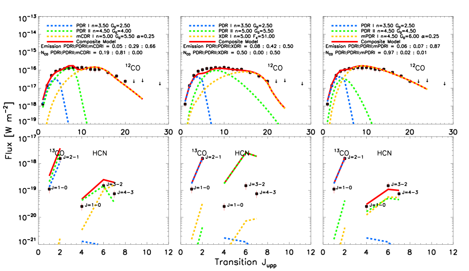
Figure 9: ¹²CO (top), ¹³CO, and HCN (bottom) excitation ladders of Arp 299 A with the flux of each transition plotted as black asterisks with red error bars. In blue, green and yellow dotted lines we plot the PDR/PDR/mCDR (left), PDR/PDR/mPDR (center), and PDR/PDR/XDR(right) ISM phases with their filling factors. The composite model is plotted with a red solid line. The model H₂ density [log cm^-3], $G/$G₀ [log Habing flux] or F_X [log erg s^-1 cm^-2], and percentage mechanical heating ($\alpha$) are shown in the legend along with the relative contribution of each phase in terms of emission and column density. For emission, we compared the integrated intensity of each ISM phase to the total modeled CO flux (the red line). For the column density we perform the same calculation except comparing the column density of each phase to the total combined model column density.

Table 5: Model parameters for the three ISM phases for each of the three cases.

Component	Density log(nH)	log($G$)	log(NCO)	log(N${}_{H_{2}}$)	$\alpha$	$\Omega$	Cem	C${}_{N_{CO}}$	Mass${}_{N_{H_{2}}}$
	log[cm-3]	G0	log[cm-2]	log[cm-2]	%				M⊙
Case 1 Mtot: $3\times 10^{9}$ M⊙
PDR I	3.5	2.5	17.1	21.5	0	0.9	0.05	0.19	$2\times 10^{9}$
PDR II	4.5	4.0	18.2	21.9	0	0.3	0.29	0.81	$1\times 10^{9}$
mCDR I	5.0	5.5	17.2	21.0	25	0.006	0.66	$<0.01$	$3\times 10^{6}$
Case 2 Mtot: $4\times 10^{9}$ M⊙
PDR I	3.5	2.5	17.1	21.5	0	1.2	0.11	0.50	$2\times 10^{9}$
PDR II	5.0	5.5	14.9	21.2	0	1.2	0.40	0.003	$1\times 10^{9}$
XDR I	5.0	51.0	19.4	23.4	0	0.006	0.48	0.50	$1\times 10^{9}$
Case 3 Mtot: $3\times 10^{9}$ M⊙
PDR I	3.5	2.5	17.1	21.5	0	1.2	0.06	0.97	$2\times 10^{9}$
PDR II	4.5	4.5	15.5	21.4	0	0.8	0.07	0.02	$1\times 10^{9}$
mPDR I	4.5	6.0	15.7	19.5	25	0.3	0.87	$<0.01$	$6\times 10^{6}$

5.3.1 Case 1

In this case, the best fit is two PDRs and one mechanically heated CDR (mCDR) with 25% mechanical heating at the surface. We also tried a fit with one, two, and three pure CDRs. The case of one CDR is the best of those options, yet has the same model parameters as the three PDR fits. This suggests that it is still the UV photons that are heating the gas instead of a strong contribution from the cosmic rays. In addition, in the case of one pure CDR, the HCN is overproduced by an order of magnitude, as in the three PDR fit. Thus, we concentrate on the overall best fit using an enhanced cosmic ray ionization rate and with 25% mechanical heating. This model is able to fit all ¹²CO transitions within the error bars. However, the second and third ISM phases (green and yellow) produce more HCN luminosity than we observe. The ¹³CO is also poorly fit, overproducing not only the J=1-0 but also the J=2-1 transition, thus making this an overall poor fit. We suggest that cosmic rays play an unimportant role in heating the molecular gas in Arp 299 A, especially since the model needs 25% mechanical heating in order to fit the high-J CO transitions.

5.3.2 Case 2

The second case that includes X-ray heating is justified by the existence of an AGN in Arp 299 A that could be heating a molecular torus around the AGN. However, HCN is very poorly fit. In order for an XDR to produce the high-J CO lines, it does not produce much emission in the mid-J CO lines. This means that the mid-J CO lines must be produced by a powerful and dense PDR that results in bright HCN emission. Thus, the best fitting XDR model is the one that can reproduce most of the high-J CO lines while producing minimal HCN emission. This points to the fact that XDR chemistry is unlikely to be the cause of the observed high-J CO emission. If it were responsible for the high-J CO emission, the third ISM phase would be the most massive one. The mass of the XDR phase exceeds the total measured molecular mass for the entire system, and thus we rule out X-rays as a significant heating source of the gas.

5.3.3 Case 3

Case 3 represents two PDRs and one mechanically heated PDR. This case is the only case that fits all observed transitions within the error bars. We also attempted to fit the observed transitions with one, two, and three mPDRs, yet in the case of two mPDRs, one of them has negligible mechanical heating, and in the case of three mPDRs there is no reasonable fit. Thus, the situation represents a galaxy in which most of the gas is heated by UV photons, but a small amount of gas is heated almost entirely by mechanical heating. This gas could be in pockets of violent star formation where the stellar winds, jets, and/or supernovae are creating turbulence that efficiently couples to the gas. The heating rate of the mechanical heating is $7.9\times 10^{-19}$ erg s^-1 cm^-2, which represents $\sim 4\%$ of the total heating, reflecting the fact that in this system the mechanical heating is very localized. We conclude that mechanical heating is the most likely candidate for the additional heating source in Arp 299 A.

This result is similar to what was found in NGC 253 (Rosenberg et al. 2014; Hailey-Dunsheath et al. 2008), where mechanical heating is needed as an additional heating mechanism. However, in NGC 253, the system requires mechanical heating in all three ISM phases to reproduce the extremely bright CO emission. Since Arp 299 A only needs mechanical heating to explain the third, most extreme, ISM phase, this lends itself to isolated and localized mechanical heating deriving from either supernova remnants or extreme star formation regions with powerful winds. The nuclear region of NGC 253 on the other hand, has universally bright CO lines, meaning the mechanical heating must be distributed throughout the galactic nucleus, perhaps coming from the massive molecular outflow (Bolatto et al. 2013; Turner & Ho 1985). In addition, although the far-infrared luminosity in Arp 299 is about an order of magnitude higher than in NGC 253, we see much brighter cooling lines in NGC 253. This is most likely due to a distance effect. With SPIRE’s beam size, in NGC 253 we observe only the nuclear region, while in Arp 299 A we observe the nucleus and surrounding disk. Thus the extreme environment of the galactic nucleus is averaged out with the less luminous disk regions in Arp 299.

5.4 Molecular gas mass

We can estimate the mass of each molecular gas ISM phase as well as the total molecular gas mass for each case using Equation 4. We find a total molecular mass equal to $3\times 10^{9}$ M_⊙ regardless of excitation mechanism, which is in good agreement with the literature values. In addition, using the dust mass of 1.1$\times 10^{8}$ M_⊙, we find a gas to dust ratio of $\sim 30$. The first ISM phase is well constrained in all cases; the mass is $2\times 10^{9}$ M_⊙, making it the most massive component in most cases. The second ISM phase is also well constrained with a mass of $1\times 10^{9}$ M_⊙. The third ISM phases’ mass is not as well constrained, yet it is the least massive component in most cases, ranging from $3-6\times 10^{6}$ M_⊙, except in the case of the XDR, where this phase is more massive, $1\times 10^{9}$ M_⊙.

The fact that the mass is so well constrained underlines the importance of observing even just two ¹³CO transitions. We also see the strength of including HCN measurements to constrain both the high density ISM phase, and the excitation mechanism. Further, these results agree with those from Rosenberg et al. (2014) that mechanical heating plays an important role in understanding the molecular line emission, even though UV heating is still the most dominant heating source.

6 Limitations and usefulness of the ¹²CO ladder

Herschel SPIRE gave access to the full CO ladder ranging from J=4-3 to J=13-12, in the nearby universe. With Herschel PACS, higher J lines could also be observed. Before Herschel, it was thought that observing the flux of CO transitions greater than J=10 would break the degeneracy between UV excitation and X-ray excitation. However, now that the wealth of observations from the Herschel Space Observatory are available, access to the full CO ladder does not necessarily break this degeneracy. In fact, the information that can be extracted from observations of only ¹²CO is very limited.

Qualitatively, bright ¹²CO emission indicates the presence of warm molecular gas. However, without any other information, the source of heating, the amount (mass) of heated gas, and the precise density and temperature cannot be determined. It is possible, however, to extract the turnover point of the ¹²CO. If the turnover point is in the low to mid-J transitions (from J=1-0 to J=6-5), as seen in Arp 299 B+C, the gas is most likely heated by UV photons in PDRs. If the turnover is higher than that, it can be either an extreme PDR ($n_{H}>10^{5}$ cm^-3, $G>10^{5}$ G₀), X-rays, cosmic rays, or mechanical heating that may be responsible. This is demonstrated fitting a pure PDR model to the high-J CO lines, and is clear in the degeneracy parameter space diagrams shown in Figure 3 by Rosenberg et al. (2014).

For metal-rich extragalactic sources, the ¹²CO ladder represents all the molecular clouds in the galaxy, spanning a range of physical environments. Therefore, multiple ISM phases are necessary to fit the ladder. These ISM phases represent many clouds with similar physical properties. In addition, with just transitions of ¹²CO, you can determine distinct density-temperature combinations for each phase. In general, the low-J CO lines are from a lower density, lower temperature ISM phase, but the density-temperature combination is highly degenerate. The mid-J CO transitions arise from a warm and medium density phase, and the high-J transitions from a high density, high temperature phase.

If multiple transitions of ¹³CO are added, then the beam averaged optical depth, and thus column density, are constrained. This allows for a better constrained mass estimate. It also helps lessen the temperature-density degeneracy, but does not break it. In order to break this degeneracy, other molecules must be added. For example, HCN, HNC, and HCO⁺ are good tracers of density for high density environments. For lower density regimes, [CI] can be a good probe of the gas temperature, yet it is very difficult to interpret, since we cannot disentangle different emitting regions within our beam. To summarize, if bright ¹²CO emission is observed, there is warm gas. Yet in order to probe the physical parameters of that gas, other molecular information is crucial. Some of these molecules do not always originate from the same spatial location as the ¹²CO and may be tracing a different gas component altogether. Interpreting ¹²CO is not trivial and the analysis should be performed with an understanding of the challenges and limitations.

Many Herschel SPIRE CO ladders have been obtained from luminous infrared galaxies, and they all require some additional heating mechanism to explain the high-J CO emission. For example in Arp 220, Rangwala et al. (2011) find that PDRs, XDRs, and CDRs can be ruled out, while the mechanical energy available in this galaxy is sufficient to heat the gas. Similarly, Meijerink et al. (2013) find strong evidence for shock heating in NGC 6240. On the other hand, Spinoglio et al. (2012) and van der Werf et al. (2010) find in NGC 1068 and Mrk 231 respectively, that it is likely XDR heating responsible for the high excitation CO lines. Although both of these sources have confirmed AGN, the CO ladder fitting was not combined with a dense gas tracer (HCN/HNC/HCO⁺), and thus mechanical heating cannot be directly ruled out. The picture emerging from the SPIRE CO-ladders is that in these extreme star forming galaxies, the gas is rarely heated by only UV photons and that in most cases, the molecular gas is heated through either X-rays or mechanical heating.

7 Conclusions

We observed Arp 299 with Herschel PACS and SPIRE in both the spectrometer and photometer mode. The Herschel SPIRE FTS observations had three separate pointings, namely towards Arp 299 A, B and C. The pointings of Arp 299 B and C are overlapping so it is difficult to separate the emission from each nucleus. We extract the line fluxes of the CO transitions, [CI], [NII], and bright H₂O lines for Arp 299 A, B, and C separately. We also measure the continuum fluxes from SPIRE photometer mode at 250, 350, and 500 $\mu$m. With PACS, we detect CO transitions from J=14-13 to 20-19 and upper limits up to J=28-27. Using these data, we find:

1. A simple quantitative comparison of the spectra of Arp 299 A with B and C shows that the environment of source A is much more excited, with more warm molecular gas.

2. Using the full range of CO transitions we construct CO excitation ladders for each of the three pointings. Again, the CO ladders reveal a clear disparity between Arp 299 A and B+C; source A displays a flattened ladder, while B+C turns over around J=5-4.

3. Since we have high-J ¹²CO PACS observations along with ¹³CO and HCN JCMT observations of Arp 299 A, we perform an automated $\chi^{2}$ minimized fitting routine to fit the CO and HCN ladders with three ISM components. We find a suitable fit for ¹²CO and ¹³CO but not for HCN. In addition, the third ISM phase would then be a truly extreme PDR, an order of magnitude more extreme than Orion Bar.

4. We create an infrared SED using values from the literature along with PACS and SPIRE continuum measurements. We fit this SED with three gray bodies and determine the temperature and mass of each dust component (cold, warm, and hot). We do not observe enough hot dust to match the amount of hot dust that would then be produced by the extreme PDR, in the case of a fit by three pure PDRs. Thus, we conclude that the flattening of the CO ladder, and extra excitation of the ¹²CO in Arp 299 A in comparison to B+C, is due to an additional heating mechanism.

5. We allow the third ISM phase (high density, high excitation) to have additional heating by cosmic rays, mechanical heating, and X-rays. We find mechanical heating to be the most likely additional heating source since it fits all transitions within the errors. As the best fit model requires mechanical heating only in the third component, this suggests that for Arp 299A the mechanical heating is localized, likely to come from supernovae remnants or pockets of intense star formation.

6. We caution the use of ¹²CO alone as a tracer of the physical conditions of the ISM. We find that ¹²CO reveals only the presence of warm molecular gas, but that the amount, physical properties, and heating source cannot be determined without observations of other molecules.