Entropy Production of Open Quantum System in Multi-Bath Environment

Abstract

We study the entropy production of an open quantum system surrounded by a complex environment consisting of several heat baths at different temperatures. The detailed balance is elaborated in view of the distinguishable channels provided by the couplings to different heat baths, and a refined entropy production rate is derived accordingly. It is demonstrated that the entropy production rates can characterize the quantum statistical property of the baths: the bosonic and fermionic baths display different behaviors in the high-temperature limit while they have the same asymptotic behavior at low temperature.

Introduction.—The concept of entropy plays an important role in our understanding of complex physical systems. For a closed system its entropy will never decrease if the unitarity condition is satisfied whether the system enjoys time reversal invariance or not Yang 1980 ; Thomsen 1953 . For an open system contacting with its environment entropy production is a pivotal concept. The so called entropy production rate (EPR) is usually regarded as a signature of the irreversibility associated with such a system Prigogine1977 . In fact, EPR is a proper physical quantity tagging the steady state of an open system. A lot of open systems can be well studied in the framework of time-homogeneous Markov process. The steady states of such systems fall into two categories: equilibrium steady states and non-equilibrium ones. In a non-equilibrium steady state the detailed balance is broken, or equivalently, the EPR does not vanish. Thus one can say that the system is in an equilibrium steady state if and only if the accompanying EPR is zero.

It should be noted that from purely mathematical point of view the reversibility of a time-homogeneous Markov process and the detailed balance condition has been thorough studied by Kolmogorov Kolmogorov1936 .

For a Markov process determined by the Pauli master equation $\dot{p}_{i}=\sum_{j}p_{j}L_{ji}-p_{i}L_{ij}$, the breaking of detailed balance is quantitively characterized by a non-vanishing EPR Schnakenberg1976 ; M Qian2012 ; M Qian 2004 ; Spohn1978

$$R=\frac{1}{2}\sum_{ij}(p_{i}L_{ij}-p_{j}L_{ji})\ln\frac{p_{i}L_{ij}}{p_{j}L_{ji}}.$$ (1)

Here, $p_{j}$ is the probability of the open system with which the open system appears in state-$j$ and $L_{ij}$ is the transition rate from state-$i$ to state-$j$. If the detailed balance is satisfied, i.e., $p_{i}L_{ij}=p_{j}L_{ji},$ there is no entropy production when the system reaches the steady state. This observation has been the starting point of a fruitful study of some non-equilibrium biochemical reactions (see Ref. M Qian 2000 and references therein).

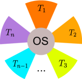
Figure 1: (color online). A complicated non-equilibrium process of an open system (OS) contacting with $n$ heat baths, where the temperature of the $i$-th heat bath is $T_{i}$.

The above formula of EPR is valid for a classical system contacting with a single canonical heat bath. For the system in a complex environment consisting of two or more heat baths at different temperatures (see Fig. 1), which allows more complicated non-equilibrium processes Esposito 2007 , the formula should be generalized. In fact, if the conventional EPR formula (1) were applied in this case, we would obtain a vanishing EPR whenever the system reaches the steady state. This contradicts the intuitional physical picture. We notice that the non-equilibrium processes induced by the multi-bath environment emerge in many practical systems, such as an opto-mechanical system with quantum cavity field coupled to two moving cavity wells at different temperatures H Ian2008 , and a quantum dot system gated by two electrodes Gurvitz1998 ; Esposito 2009 at different temperatures.

In this letter, we first derive a quantum EPR formula for the above mentioned multi-bath case from the master equation of the open quantum system. When the quantum coherence is neglected, our general result reduces to the multi-channel expression of EPR as given in Ref. Esposito 2007 . Then we show that the EPRs of non-equilibrium systems with bosonic and fermionic baths have a similar behavior at low temperature but behave quite differently in the high temperature region. This leads to the conclusion: non-equilibrium process is important as it can characteristically reflect the quantum statistical property of the bath.

Entropy Production Rate for Open Quantum Systems.—The Markovian evolution of an open quantum system in contact with its environment is described by a dynamical semigroup $\Lambda_{t}$. To be precise, we have $\rho(t)=\Lambda_{t}\rho(0)$ and the density matrix $\rho(t)$ satisfies the master equation $\dot{\rho}={\cal L}[\rho]$ with Lindblad super-operator ${\cal L}$ (we always work in the interaction picture hereafter) Lindblad 1976 . For a heat bath at temperature $T$, it has been shown that the EPR can be formulated by the relative entropy as $R^{(0)}=-\frac{\mathrm{d}}{\mathrm{d}t}S(\rho||\rho^{\mathrm{th}})$Spohn1978 ; Breuer2002 . Here, the reference state $\rho^{\mathrm{th}}=\exp[-\beta H]/Z$ is the steady state given by ${\cal L}[\rho^{\mathrm{th}}]=0$, and it is the thermal equilibrium state at the temperature $T=\beta^{-1}$. The EPR formula is decomposed into two terms, one of which is $-\frac{\mathrm{d}}{\mathrm{d}t}\mathrm{tr}[\rho\ln\rho]$, representing the entropy changing rate of the open system itselfand the other of which takes the form:

$$\frac{\mathrm{d}}{\mathrm{d}t}\mathrm{tr}(\rho\ln\rho^{\mathrm{th}})=\frac{\mathrm{d}}{\mathrm{d}t}\mathrm{tr}[\rho(-\beta H)]=-\frac{1}{T}\frac{\mathrm{d}\left\langle H\right\rangle}{\mathrm{d}t}.$$ (2)

Since $-\frac{\mathrm{d}}{\mathrm{d}t}\left\langle H\right\rangle:=\dot{Q}$ is the rate of the heat dissipating into the heat bath HT Quan2005 , this term describes the entropy changing rate of the heat bath. Thus this EPR formula actually counts the total entropy changing rate of both the open system and its environment.

For an open quantum system interacting with $N$ reservoirs (Fig. 1), the master equation assumes the form $\dot{\rho}=\sum_{l=1}^{N}{\cal L}_{l}[\rho]$, where ${\cal L}_{l}$ is the Lindblad super-operator corresponding to the $l$-th reservoir. In time interval $\mathrm{d}t$, the energy dissipating into reservoir-$l$ is $\mathrm{\mkern 3.0mu\mathchar 22\relax\mkern-12.0mud}Q_{l}:=-\mathrm{tr}\big{[}{\cal L}_{l}[\rho]H\big{]}\mathrm{d}t$ HT Quan2005 , thus the entropy changing rate through the $l$-th reservoir is

$$\frac{\dot{Q}_{l}}{T_{l}}=-\frac{1}{T_{l}}\mathrm{tr}\big{[}{\cal L}_{l}[\rho]H\big{]},$$ (3)

where $\rho_{l}^{\mathrm{th}}:=\exp[-\beta_{l}H]/Z_{l}$ is the thermal state of reservoir-$l$ with temperature $\beta_{l}^{-1}$. Then the entropy production rate for a non-equilibrium quantum system is obtained as $R=\frac{\mathrm{d}}{\mathrm{d}t}\mathrm{tr}[\rho\ln\rho]+\sum_{l}\dot{Q}_{l}/T_{l}$, i.e,

$$R=-\sum_{l=1}^{N}\mathrm{tr}\big{[}{\cal L}_{l}[\rho](\ln\rho-\ln\rho_{l}^{\mathrm{th}})\big{]},$$ (4)

which represents the total entropy changing rate of the open system and its multi-bath environment. It has been proved that the quantity $R_{l}:=-\mathrm{tr}\big{[}{\cal L}_{l}[\rho](\ln\rho-\ln\rho_{l}^{\mathrm{th}})\big{]}$ is non-negative Spohn1978 , so we always have $R=\sum_{l}R_{l}\geqslant 0$.

The dynamics of the quantum coherence is usually decoupled from that of the populations (when we say quantum coherence, we mean the effect contributed from the off-diagonal terms $\langle i|\rho|j\rangle$ of $\rho$ in the eigen energy representation) Breuer2002 . When the quantum coherence is neglected (the effect of the quantum coherence will be studied later), the Lindblad equation reduces to Pauli master equation, and the above Eq. (4) reduces to

$$R\simeq-\sum_{l=1}^{N}\sum_{i}\langle{i}|{\cal L}_{l}[\rho]|{i}\rangle\langle{i}|(\ln\rho-\ln\rho_{l}^{\mathrm{th}})|{i}\rangle.$$ (5)

Replacing $\langle{i}|{\cal L}_{l}[\rho]|{i}\rangle$ by $\sum\limits_{j}(p_{j}L_{ji}^{(l)}-p_{i}L_{ij}^{(l)})$, we obtain

$$R=\frac{1}{2}\sum_{l=1}^{N}\sum_{i,j}(p_{j}L_{ji}^{(l)}-p_{i}L_{ij}^{(l)})(\ln\frac{p_{i}}{p_{j}}+\frac{E_{i}-E_{j}}{T_{l}})$$

Here $L_{ij}^{(l)}$ is the transition rate from state-$i$ to state-$j$ resulted from the coupling to the $l$-th heat bath, and we have used the fact that $\langle{i}|\rho_{l}^{\mathrm{th}}|{i}\rangle=\exp(-E_{i}/T_{l})/Z_{l}$. Considering the microscopic reversibility condition $L_{ij}^{(l)}/L_{ji}^{(l)}=\exp[(E_{i}-E_{j})/T_{l}],$ we then have

$$R=\frac{1}{2}\sum_{i\not=j}\sum_{l=1}^{N}(p_{i}L_{ij}^{(l)}-p_{j}L_{ji}^{(l)})\ln\frac{p_{i}L_{ij}^{(l)}}{p_{j}L_{ji}^{(l)}},$$ (6)

a refined entropy production rate. This is the same as Eq. (10) in Ref. Esposito 2007 . If the quantum coherence is taken into account, there would be extra entropy production.

Note that in the above refined entropy production rate (REPR) transitions caused by different heat baths (see Fig. 2) are treated separately while in the spirit of the conventional EPR Eq. (1) they should be merged. This essential difference naturally leads to different understandings of equilibrium state.

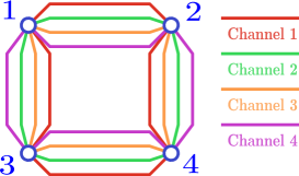
Figure 2: (color online). The transition diagram of a four-level system contacting with four heat baths. We use different colors to distinguish the channels corresponding to different heat baths.

Elaborate Detailed Balance and Time Reversibility.—As we have argued above, if the environment is composed of two or more heat baths, the REPR (6), instead of the conventional EPR Eq. (1), should be used to investigate the entroy production problem. Then, the condition for zero EPR is refined as

$$p_{i}L_{ij}^{(l)}=p_{j}L_{ji}^{(l)}.$$ (7)

This condition is subtler than the detailed balance condition $p_{i}L_{ij}=p_{j}L_{ji}$ and justifies the name of elaborate detailed balance (EDB). The quantity $L_{ij}^{(l)}$ can be viewed as the transition rate from state-$i$ to state-$j$ through the $l$-th channel. From this point of view, the EDB requires not only the balance of transitions between any two states of the system, but also the balance of each transition channel. This property has been suggested by Lewis as a criterion for equilibrium Lewis 1925 .

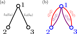
Figure 3: (color online). The transition diagram of a $\Lambda$-type system contacting with two heat baths. (a) A rough description of the system’s possible transitions, $1\leftrightarrow 2$ and $1\leftrightarrow 3$. (b) Each transition in (a) may be further divided into two channels, each of which corresponds to a transition caused by a certain heat bath.

Let us probe further the concept of transition channel with the case of a $\Lambda$-type system contacting with two heat baths. We consider the transition from state-1 to state-2, which releases energy of amount $\omega_{12}$ to its environment. If there appears an energy increase of $\omega_{12}$ in the first heat bath, then it can be judged that this transition results from the first heat bath. Thus it is physically justified to understand the transition as realized through two distinguishable channels, each of which corresponds to a transition caused by a certain heat bath. As a consequence of the validity of the concept of distinguishable channels it can be argued that a transition chain like $\cdots 1\rightarrow 2\rightarrow 1\rightarrow 3\cdots$ is not a complete description. A complete description should be something like $\cdots 1\stackrel{{\scriptstyle(1)}}{{\longrightarrow}}2\stackrel{{\scriptstyle(2)}}{{\longrightarrow}}1\stackrel{{\scriptstyle(2)}}{{\longrightarrow}}3\cdots$, where $1\stackrel{{\scriptstyle(1)}}{{\longrightarrow}}2$ denotes a transition from state-1 to state-2 via the first channel and $1\stackrel{{\scriptstyle(2)}}{{\longrightarrow}}3$ denotes a transition from state-1 to state-3 via the second channel. All the possible channels together make up a transition diagram as shown in Fig. 3b.

Under certain conditions the equivalence between the conventional detailed balance and the time reversibility of a Markov process has been proved by Kolmogorov Kolmogorov1936 . As there is no generic way to model the evolution of the open system with distinguishable transition channels as a mathematically well defined Markov process, Kolmogorov’s result is not immediately applicable to the open system with two or more baths. Nevertheless, from physical intuition, one may well expect that the time reversibility of such systems requires that the likelihood of transitions $1\stackrel{{\scriptstyle(2)}}{{\longrightarrow}}3$ be the same in the forward process and backward process: $p_{1}L_{13}^{(2)}=p_{3}L_{31}^{(2)}$. Furthermore, it is also intuitively correct that the EDB will guarantee the time reversibility of the dynamics of such systems.

Since the open systems considered here are mesoscopic or microscopic, the evolution should be subjected to quantum dynamics. There exist mainly two kinds of quantum effects to be considered in the entropy production, related to quantum statistics and quantum coherence respectively.

Quantum Statistical Effect on Entropy Production Rate.— Let us first consider the factor of quantum statistics. Bosonic and fermionic environments are fundamental in the study of quantum open systems. Bosonic heat baths usually appear in opto-mechanical systems while fermionic ones are common in the study of quantum dots. What is the essential difference between these two basic kinds of environments? In this section we try to answer this question from entropy production point of view. Our starting point is the REPR formula (6), applied to a two-level system.

For a two-level system contacting with two heat baths, the REPR [Eq. (6)] for the steady state is

$$R=\frac{\Omega}{L_{12}+L_{21}}\cdot\frac{T_{1}-T_{2}}{T_{1}T_{2}}(L_{21}^{(2)}L_{12}^{(1)}-L_{12}^{(2)}L_{21}^{(1)}).$$ (8)

Here, we have adopted the labeling: state-$1$ and state-$2$ denote the excited state and the ground state respectively. Different kinds of environments will lead to different forms of transition rates. Specifically, the transition rates caused by the$l$-th heat bath have the following forms Breuer2002 ,

$$L_{12}^{(l)} = \gamma_{l}(1\pm N(\beta_{l})),$$ (9)

$$L_{21}^{(l)} = \gamma_{l}N(\beta_{l}),$$ (10)

where ‘$+$’ and ‘$-$’ correspond to the bosonic and fermionic cases respectively. $N(\beta)=1/(\exp(\beta\Omega)\mp 1)$ is the distribution function, and $\gamma_{l}$ is the coupling strength between the system and the $l$-th heat bath. One can verify that these transition rates satisfy the microscopic reversibility $L_{12}^{(l)}=\exp(-\beta_{l}\Omega)L_{21}^{(l)}$.

The REPRs for bosonic and fermionic environments can be calculated directly. The results are

$$R_{\mathrm{boson}} =\frac{\Omega\gamma_{1}\gamma_{2}}{\gamma_{1}(2N_{1}+1)+\gamma_{2}(2N_{2}+1)}\cdot\frac{T_{1}-T_{2}}{T_{1}T_{2}}(N_{1}-N_{2}),$$

$$R_{\mathrm{fermion}} =\frac{\Omega\gamma_{1}\gamma_{2}}{\gamma_{1}+\gamma_{2}}\cdot\frac{T_{1}-T_{2}}{T_{1}T_{2}}(N_{1}-N_{2}),$$ (11)

where $N_{l}=N(\beta_{l})$. If the two temperatures are nearly equal, $T_{1}\simeq T_{2}\simeq T$, then we have the estimation

$$R_{\mathrm{boson}} \simeq\frac{\gamma_{1}\gamma_{2}}{\gamma_{1}+\gamma_{2}}\cdot\frac{\Omega^{2}}{T^{2}}\cdot\frac{N(1+N)}{2N+1}\cdot\left(\frac{\Delta T}{T}\right)^{2},$$

$$R_{\mathrm{fermion}} \simeq\frac{\gamma_{1}\gamma_{2}}{\gamma_{1}+\gamma_{2}}\cdot\frac{\Omega^{2}}{T^{2}}\cdot N(1-N)\cdot\left(\frac{\Delta T}{T}\right)^{2}.$$ (12)

In this case both of the entropy production rates are proportional to the square of $\Delta T/T$. Thus, the entropy production rate can be regarded as a response to the “driving force” $(\Delta T/T)^{2}$, and the ratio between the response and the “driving force” $C=R/(\Delta T/T)^{2}$ as a “conductance” in some sense Onsager 1930 . In the low temperature region, the “conductances” corresponding to bosonic and fermionic environments have the same asymptotic behavior:

$$C_{\mathrm{boson/fermion}}\simeq\frac{\gamma_{1}\gamma_{2}}{\gamma_{1}+\gamma_{2}}\cdot\frac{\Omega^{2}}{T^{2}}\mathrm{e}^{-\frac{\Omega}{T}}.$$ (13)

They both exponentially decays to zero as $T\rightarrow 0$. In the high temperature region, a remarkable difference arises. In this region we have

$$C_{\mathrm{boson}} \simeq\frac{\gamma_{1}\gamma_{2}}{\gamma_{1}+\gamma_{2}}\cdot\frac{\Omega}{2T},$$

$$C_{\mathrm{fermion}} \simeq\frac{\gamma_{1}\gamma_{2}}{\gamma_{1}+\gamma_{2}}\cdot\left(\frac{\Omega}{2T}\right)^{2}.$$ (14)

Thus, the bosonic “conductance” $C_{\mathrm{boson}}\propto 1/T$ as $T\rightarrow\infty$, while the fermionic “conductance” $C_{\mathrm{fermion}}\propto 1/T^{2}$ as $T\rightarrow\infty$. Since the “conductance” $C$ tends to zero in both of the limits $T\rightarrow 0$ and $T\rightarrow\infty$, there exists a maximum conductance at a certain finite temperature $T_{m}$ (see the peak of blue line in Fig. 4). The numerical simulation results for the bosonic and fermionic environments are presented in Fig. 4. It is clearly illustrated that the conductances, namely, the ratio between REPR and $(\Delta T/T)^{2}$, are indeed different for bosonic and fermionic environments, especially in the high temperature region.

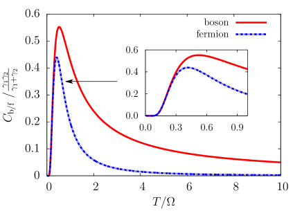
Figure 4: (color online). The ratio $C$ between the refined entropy production rate $R$ and $(\Delta T/T)^{2}$ vs the temperature $T$. The red solid line corresponds to the boson case while the blue dashed line corresponds to the fermion case. Both cases have the same behavior in the low temperature region. In the high temperature region the ratio $C$ is proportional to $1/T$ in the boson case, while it is proportional to $1/T^{2}$ in the fermion case. The peaks of the two curves correspond to the maximum conductances in boson case and fermion case respectively.

Quantum Coherence Effect on Entropy Production Rate.— Now we consider the factor of quantum coherence. Hereafter, for simplicity we assume the Markovian property of the dynamics of the quantum open system and the validity of the rotating wave approximation to the quantum master equation. Under this assumption, the evolutions of the diagonal and the off-diagonal parts of the open system’s density matrix are decoupled Breuer2002 . In other words, ${\cal L}_{l}[\rho_{coh}]$ should have vanishing diagonal elements. Here, $\rho_{coh}$ is the off-diagonal part of the density matrix, which represents the quantum coherence of the open system. Thus, $\mathrm{tr}\big{[}{\cal L}_{l}[\rho_{coh}]\,\ln\rho_{l}^{\mathrm{th}}\big{]}$ vanishes. This means that the quantum coherence exerts no influence on the heat flow between the open system and its environment. The entropy change of the open system $-\mathrm{d}\mathrm{tr}[\rho\ln\rho]/\mathrm{d}t$ can be divided into two parts:

$$-\frac{\mathrm{d}}{\mathrm{d}t}\mathrm{tr}[\rho\ln\rho]=-\mathrm{tr}[\frac{\mathrm{d}\rho_{dia}}{\mathrm{d}t}\ln\rho]-\mathrm{tr}[\frac{\mathrm{d}\rho_{coh}}{\mathrm{d}t}\ln\rho],$$ (15)

where $\rho_{dia}$ is the diagonal part of the density matrix. Correspondingly, the REPR in Eq.(4) can be divided into two parts:

$$R = \left(-\frac{\mathrm{d}}{\mathrm{d}t}\mathrm{tr}[\rho_{dia}\ln\rho]+\sum_{l=1}^{N}\mathrm{tr}\big{[}{\cal L}_{l}[\rho_{dia}]\,\ln\rho_{l}^{\mathrm{th}}\big{]}\right)$$ (16)

$$-\mathrm{tr}[\frac{\mathrm{d}\rho_{coh}}{\mathrm{d}t}\ln\rho].$$

When $t$ is larger than the time scale of the decoherence, we have $\rho\simeq\rho_{dia}$ and the term in the first line of the above equation is none other than the entropy production rate due to the diagonal part of the quantum open system, which is equal to the classical REPR inEq.(6) as we have pointed out before. The term in the second line can be interpreted as the entropy production rate due to the evolution of the off-diagonal part of the quantum open system. Thus we reach the qualitative conclusion that quantum coherence effect contributes an additional part to the entropy production.

To quantitatively study the effects of quantum coherence, let us concretely analyze a two-level system coupled with a single heat bath. The Markovian quantum master equation of this open system reads Breuer2002

$$\frac{\mathrm{d}\rho}{\mathrm{d}t} = \Gamma_{-}(\sigma_{-}\rho\sigma_{+}-\frac{1}{2}\sigma_{+}\sigma_{-}\rho-\frac{1}{2}\rho\sigma_{+}\sigma_{-})$$ (17)

$$+ \Gamma_{+}(\sigma_{+}\rho\sigma_{-}-\frac{1}{2}\sigma_{-}\sigma_{+}\rho-\frac{1}{2}\rho\sigma_{-}\sigma_{+}),$$

where $\sigma_{+}=|{\mathrm{e}}\rangle\langle{\mathrm{g}}|,\ \sigma_{-}=|{\mathrm{g}}\rangle\langle{\mathrm{e}}|,$ are the raising and lowering operators of the two-level system respectively. The evolution of the off-diagonal elements $\rho_{\mathrm{eg}}(t)=\mathrm{exp(-\Gamma t/2)}\rho_{\mathrm{eg}}(0),$ as expected, is decoupled from the diagonal part of the system where $\Gamma=\Gamma_{+}+\Gamma_{-}$ is the inverse evolution timescale of the off-diagonal part. Thus the entropy production due to the quantum coherence effect is

$$R_{con}=-\frac{1}{\alpha(t)}\ln\frac{1+\alpha(t)}{1-\alpha(t)}\frac{\mathrm{d}|\rho_{\mathrm{eg}}|^{2}}{\mathrm{d}t},$$ (18)

where

$$\alpha(t)=\sqrt{\left(\frac{\Gamma_{-}-\Gamma_{+}}{\Gamma_{-}+\Gamma_{+}}\right)^{2}+4|\rho_{\mathrm{eg}}|^{2}}.$$ (19)

For a long-time evolution such that $|\rho_{\mathrm{eg}}|\ll(\Gamma_{-}-\Gamma_{+})/\Gamma$, $R_{con}$ can be estimated as

$$R_{con}\backsimeq\Gamma\beta\Omega\coth\frac{\beta\Omega}{2}\mathrm{e}^{-\Gamma t}|\rho_{\mathrm{eg}}(0)|^{2}.$$ (20)

It decays exponentially as $t\rightarrow\infty$.

If initially the diagonal part has already reached its stable value, the entropy production rate due to the diagonal part of the quantum open system would remain vaninishing in the evolution. Thus, if we can “kick” an open system, which has been already stabilized to a thermal state, so that its off-diagonal part becomes non-zero while its diagonal part remains “untouched” , we may be able to observe the entropy production due to the quantum coherence effect.

Conclusions and Discussions.— In this letter, we try to probe open quantum systems in contact with two or more baths from entropy production point of view. We derive a refined formula for the entropy production rate for such systems. This foumula can well reflect the effects of statistics and quantum coherence on the entropy production. In the two-bath case, it turns out that the REPRs in bosonic and fermionic environments are proportional to the square of temperature difference $(\Delta T/T)^{2}$ between the two heat baths, but the behaviors of the so called conductances are quite different in the high temperature region. This reveals a connection between the entropy production of the open quantum system and the quantum statistical property of the baths. The results in this letter are applicable to a non-equilibrium system weakly coupled to its environment. If the system-bath coupling is too strong or the coupling spectrum has some exotic structure, the non-Markovian effects may dominate the long-time behavior of the systems Cai 2013 , and the entropy production behavior for such non-Markovian processes deserves further investigations.

This work was supported by the National Natural Science Foundation of China (Grant No. 11121403) and the National 973 program (Grant No. 2012CB922104 and No. 2014CB921403).

References

- (1) C. N. Yang and C. P. Yang , Trans. NY Acad. Sci. 40, 267 (1980).
- (2) J. S. Thomsen, Phys. Rev. 91,1263 (1953).
- (3) G. Nicolis, I. Prigogine, Self-organization in Non-equilibrium Systems: From Dissipative Structures to Order Through Fluctuation, Wiley, New York, 1977.
- (4) A. N. Kolmogorov, Math. Ann. 112, 155 (1936).
- (5) J. Schnakenberg, Rev. Mod. Phys. 48, 571–585 (1976).
- (6) X. J. Zhang, H. Qian, and M. Qian, Physics Reports 510, 1 (2012).
- (7) D. Q. Jiang, M. Qian, and M. P. Qian, Mathematical Theory of Non-equilibrium Steady States, in: Lecture Notes in Mathematics, vol. 1883, Springer-Verlag, Berlin, 2004.
- (8) H. Spohn, J. Math. Phys. (N.Y.) 19, 1227 (1978).
- (9) H. Qian and M. Qian, Phys. Rev. Lett. 84, 2271 (2000).
- (10) M. Esposito, U. Harbola, and S. Mukamel, Phy. Rev. E, 76, 031132 (2007).
- (11) H. Ian et al., Phys. Rev. A 78, 013824 (2008).
- (12) S. A. Gurvitz, Phys. Rev. B 57, 6602–6611 (1998).
- (13) M. Esposito, K. Lindenberg, and C. Van den Broeck, Europhys. Lett. 85, 60010 (2009).
- (14) G. Lindblad, Commun. math. Phys. 48, 119 (1976).
- (15) H. P. Breuer and F. Petruccione, The Theory of Open Quantum Systems, Oxford University Press, New York, 2002.
- (16) H. T. Quan, P. Zhang, and C. P. Sun, Phys. Rev. E 72, 056110 (2005).
- (17) G. N. Lewis, Proc. Natl. Acad. Sci. USA 11 179 (1925).
- (18) L. Onsager Phys. Rev. 37, 405 (1930).
- (19) C. Y. Cai, L. P. Yang, and C. P. Sun, Phys. Rev. A 89, 012128 (2014).