Two-point correlation functions of QCD in the Landau gauge

Abstract

We investigate the gluon, ghost and quark propagators in the Landau gauge with dynamic quarks. We perform a one-loop calculation in a model where the standard Faddeev-Popov Lagrangian is complemented by a mass term for the gluons which is seen as a minimal way of taking into account the effect of the Gribov copies. The analytic results are compared with lattice data obtained in four dimension and for two, three and four quark flavors. The gluon and ghost propagators are reproduced with a few percent accuracy in the whole range of accessible momenta. The scalar part of the quark propagator is found to be in good agreement with the lattice data. However, the quark renormalization is poorly described. We attribute this discrepancy to the fact that the one-loop corrections to this quantity are unusually small so that the two loop contribution can not be discarded. The results are expressed in terms of the coupling, the gluon mass and the light quark mass at 1 GeV.

I Introduction

It is well-known that the Faddeev-Popov construction, which is the standard analytic method for fixing the gauge, is not sufficient in order to treat the infrared regime of QCD. The problem originates in the existence of Gribov copies Gribov77 which are ignored in the Faddeev-Popov construction. Gribov copies do not play any role in the ultraviolet regime. For that reason, the Yang-Mills action complemented by the Faddeev-Popov action is a good starting point to analyze both gauge-invariant and non-invariant quantities at momentum scales much bigger than $1$ GeV. However, at low momenta the question of how to include the effect of Gribov copies in a Lagrangian still remains unsolved even though some ideas have been already developed. Among those, the most popular is probably the Gribov–Zwanziger proposal Zwanziger89 ; Zwanziger92 ; Zwanziger01 ; Dudal08 . It consists in restricting the functional integral to the first Gribov region by adding several new fields. Unfortunately it was shown in vanBaal:1991zw that the first Gribov region also includes many Gribov copies so that the Gribov ambiguity is not completely removed. Moreover, the Gribov-Zwanzinger procedure relies on some formal manipulations that are not fully justified from first principles.

In the past decades, lattice simulations improved considerably and became the most reliable technique to describe the infrared region of QCD montvay94 . In particular, quenched lattice simulations in Landau gauge Sternbeck:2007ug ; Cucchieri_08b ; Cucchieri_08c ; Sternbeck:2008mv ; Cucchieri09 ; Bogolubsky09 ; Dudal10 and unquenched simulations Bowman:2004jm ; Parappilly:2006si have demonstrated that the gluon propagator acquires a finite value at low momentum, contrary to the original belief. Numerical simulations succeeded in convincing the community that, in this gauge, the gluon propagator behaves in the IR as if it was massive.

Even before that, the infrared regime was studied through several semi-analytical methods, among which the more popular were based on Dyson-Schwinger (DS) equations. Depending on the precise implementation, two solutions were observed, called scaling and decoupling (or massive) solutions. The scaling solution is characterized by a gluon propagator that vanishes as a power law at low momentum vonSmekal97 ; Alkofer00 ; Zwanziger01 ; Fischer03 ; Bloch03 ; Fischer08 . On the other hand, the decoupling solution corresponds to a finite gluon propagator Aguilar04 ; Boucaud06 ; Aguilar07 ; Aguilar08 ; Boucaud08 ; Fischer08 ; RodriguezQuintero10 ; Huber:2012kd , in agreement with lattice results.

Acknowledging the fact that no analytic method can deal with the Gribov ambiguity in a fully consistent way, two of the authors have proposed an alternative strategy to study analytically the IR regime of the theory. The idea relies on working with the simplest Lagrangian which reproduces lattice results. To account for the decoupling solution observed on the lattice in a minimal way, the Faddeev-Popov Lagrangian is complemented by a mass term for the gluons. In euclidean space, the Lagrangian density reads:

$$\begin{split}\mathcal{L}=&\frac{1}{4}F_{\mu\nu}^{a}F_{\mu\nu}^{a}+\partial_{\mu}\bar{c}^{a}(D_{\mu}c)^{a}+ih^{a}\partial_{\mu}A_{\mu}^{a}\\ &+\frac{m^{2}}{2}A_{\mu}^{a}A_{\mu}^{a}+\sum_{i=1}^{N_{f}}\bar{\psi}_{i}(\gamma_{\mu}D_{\mu}+M_{i})\psi_{i},\end{split}$$ (1)

where $g$ is the coupling constant, $\gamma_{\mu}$ are euclidean Dirac matrices satisfying $\{\gamma_{\mu},\gamma_{\nu}\}=2\delta_{\mu,\nu}$, the flavor index $i$ runs over the $N_{f}$ quark flavors and

$$F_{\mu\nu}^{a} =\partial_{\mu}A_{\nu}^{a}-\partial_{\nu}A_{\mu}^{a}+gf^{abc}A_{\mu}^{b}A_{\nu}^{c},$$

$$(D_{\mu}c)^{a} =\partial_{\mu}c^{a}+gf^{abc}A_{\mu}^{b}c^{c},$$

$$D_{\mu}\psi =\partial_{\mu}\psi-igA_{\mu}^{a}t^{a}\psi.$$

The latin indices correspond to the $SU(N)$ gauge group, $t^{a}$ are the generators of the algebra in the fundamental representation and $f^{abc}$ are the structure constants.

The model described by Eq. (1) is a particular case of the Curci-Ferrari model Curci76 . It is well known that the mass term violates the BRST symmetry of the Faddeev-Popov Lagrangian. However, it is still symmetric under a modified BRST symmetry responsible for its renormalizability. This Lagrangian can also be motivated from first principles by taking into account Gribov copies Serreau:2012cg .

A great advantage of the phenomenological model described by Eq. (1) is that it is very simple and allows to perform perturbative calculations very easily. Moreover, we found Tissier:2010ts ; Tissier:2011ey that there exist renormalization schemes in which the coupling constant remains finite at all momentum scales. The absence of Landau pole allows us to implement perturbation theory even in the infrared regime. The quenched one-loop calculations for the two-point Tissier:2010ts ; Tissier:2011ey and three-point Pelaez:2013cpa correlation functions compare very well with lattice simulations. The previous model was also used for studying the two-point correlation functions at finite temperature reinosa14 where it reproduces at a qualitative level the properties of the gluon and ghost propagators.

In this article, we pursue our systematic comparison of the correlation functions obtained within the model (1) with those extracted from lattice simulations. We include here dynamical quarks and compute, at one loop, the two-point correlation function for the gluon, ghost and quark, for arbitrary dimension, number of colors ($N$) and flavors ($N_{f}$). The rest of the article is organized as follows. In Sect. II, we discuss the 1-loop calculation for the gluon and ghost propagators which are expressed in terms of Passarino-Veltman integrals Passarino78 . We present our results in arbitrary dimension and give explicit expressions in the physically relevant case $d=4$. Sect. III is devoted to the quark propagator. In Sect. IV we introduce the renormalization schemes and discuss the implementation of the renormalization group. In Sect. V we perform a comparison of lattice correlation functions with our unquenched perturbative results in the gluon and ghost sector. We focus on $N=3$ with two light degenerates quarks ($N_{f}=2$) and with two light quarks and two heavier quarks ($N_{f}=2+1+1$). In Sect. VI we work with $N_{f}=2+1$. The quark propagator was extracted from lattice simulations in this case, which enables us to make a comparison with our analytical results. Finally, in Sect. VII we estimate the two-loop contributions which gives an indication of the error bars on our results.

II Unquenched Gluon and Ghost propagator

The gluon and ghost propagators have been extensively studied in lattice simulations, both in the quenched and unquenched case. It is found that the addition of the sea quarks does not change qualitatively the behavior of both propagators. It however tends to lower the plateau observed at small momenta for the gluon propagator.

We parametrize the gluon and ghost 2-point vertex functions in the following way

$$\Gamma^{(2)}_{A_{\mu}^{a}A_{\nu}^{b}}(p)=\delta^{ab}\big{[}\Gamma^{\perp}(p)P^{\perp}_{\mu\nu}(p)+\Gamma^{\parallel}(p)P^{\parallel}_{\mu\nu}(p)\big{]},$$ (2)

$$\Gamma^{(2)}_{c^{a}\overline{c}^{b}}(p)=\delta^{ab}\frac{p^{2}}{J(p)},$$ (3)

where $P^{\perp}_{\mu\nu}$ and $P^{\parallel}_{\mu\nu}$ are the transverse and parallel projector respectively, defined as:

$$P^{\parallel}_{\mu\nu}(p)=\frac{p_{\mu}p_{\nu}}{p^{2}}\hskip 14.22636pt\text{and}\hskip 14.22636ptP^{\perp}_{\mu\nu}(p)=\delta_{\mu\nu}-P^{\parallel}_{\mu\nu}(p).$$

In linear covariant gauges and in particular in the linear version of the Landau gauge without the inclusion of the mass term, the gluon self-energy is transverse. Here, the longitudinal part is non-zero but it is controlled by a non-renormalization theorem (see Tissier:2011ey ). It is important to stress, however, that this longitudinal part has no impact on the gluon propagator, which is transverse in Landau gauge even in presence of the mass term. Similar remarks apply to higher vertex functions, that contains longitudinal parts, but which do not contribute to the corresponding correlation functions. The function $J(p)$ (usually called the dressing function of the ghost) and the $\Gamma^{\perp}(p)$ (the transverse part of the two-point gluon vertex, related to the gluon dressing function $\frac{p^{2}}{\Gamma^{\perp}(p)}$) explicitly appear in the ghost and gluon propagators and are therefore of special interest in order to compare our calculations with lattice results. As the longitudinal part of the two-point gluon vertex is not directly accessible in lattice simulations, we do not describe it here.

At one-loop, the gluon and ghost two-point vertex functions are given by the diagrams shown in Fig. 1.

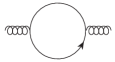
Figure 1: First line: four diagrams contributing to the gluon self-energy. Second line: diagram contributing to the ghost self-energy

Most of these diagrams were already computed in Tissier:2010ts . In what concerns the gluon propagator, we just need here to compute the diagram with a quark loop (fourth diagram of Fig. 1), which can be expressed in terms of Passarino-Veltman integrals as

$$\begin{split}\Gamma_{\text{1loop},4}^{\perp}(p)=&\frac{2g^{2}T_{f}}{(d-1)}\left\{[4M^{2}-(d-2)p^{2}]B_{0}(p,M,M)\right.\\ &\left.+2(d-2)A(M)\right\},\end{split}$$ (4)

where the index $4$ represents the fourth diagram in Fig. 1 and $T_{f}$ is defined by ${\rm Tr}(t^{a}t^{b})=T_{f}\delta^{ab}$ (in the fundamental representation, $T_{f}=1/2$). The $A$ and $B_{0}$ functions are the analogue of Passarino-Veltman integrals Passarino78 in euclidean space:

$$A(m_{1})=\int\frac{d^{d}q}{(2\pi)^{d}}\frac{1}{q^{2}+m_{1}^{2}}$$

$$B_{0}(p,m_{1},m_{2})=\int\frac{d^{d}q}{(2\pi)^{d}}\frac{1}{q^{2}+m_{1}^{2}}\frac{1}{(q+p)^{2}+m_{2}^{2}}$$

Each quark flavor contributes to the gluon vertex and it is therefore necessary to sum this diagram over the flavors, with $M$ replaced by the corresponding quark mass. We have checked that (4) coincides with the expression of davydychev96 when the quark mass is set to zero.

In $d=4-\epsilon$, the diagram can be expressed in a completely analytical form:

$$\begin{split}\Gamma_{\text{1loop},4}^{\perp}&(p)=\frac{g^{2}T_{f}p^{2}}{6\pi^{2}}\Big{\{}-\frac{1}{\epsilon}+\log\left(\frac{Me^{\gamma/2}}{\sqrt{4\pi}}\right)-\frac{5}{6}+2t\\ &+\left(1-2t\right)\sqrt{4t+1}\coth^{-1}\left(\sqrt{4t+1}\right)\Big{\}}+\mathcal{O}(\epsilon)\\ \end{split}$$

where $t=\frac{M^{2}}{p^{2}}$.

At one loop, the ghost propagator is the same as in the quenched situation due to the non-existence of a ghost-quark vertex. However, the ghost dressing function will be indirectly influenced by the quarks through the renormalization-group flow of the coupling constant and gluon mass.

III Quark propagator

The one-loop contribution to the quark two-point vertex involves only one diagram which is shown in Fig. 2. It has two independent structures in Dirac indices and is therefore parametrized by two scalar functions:

$$\Gamma^{(2)}_{\psi\bar{\psi}}(p^{2})=Z^{-1}(p)\left(i\not{p}+M(p)\right)$$

Both $M(p)$ and $Z(p)$ have been determined in lattice simulations.

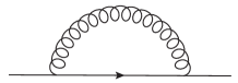
Figure 2: diagram contributing to the quark two point vertex

This diagram is expressed in terms of Passarino-Veltman integrals as follows:

$$\begin{split}\Gamma^{(2)}_{\psi\bar{\psi},\text{1loop}}&(p^{2})=g^{2}(d-1)MB_{0}(p,m,M)\\ &-i\not{p}\frac{g^{2}C_{f}}{2m^{2}p^{2}}\Big{\{}\big{[}(2-d)m^{4}+(d-3)m^{2}(M^{2}-p^{2})\\ &+(M^{2}+p^{2})^{2}\big{]}B_{0}(p,m,M)\\ &+(M^{2}+p^{2})^{2}B_{0}(p,0,M)+A(m)[(2-d)m^{2}\\ &-M^{2}-p^{2}]+(d-2)m^{2}A(M)\Big{\}},\end{split}$$

where $C_{f}$ is defined by $t^{a}t^{a}=C_{f}\openone$. (In the fundamental representation, $C_{f}=\frac{N^{2}-1}{2N}$.) The previous expression coincides with that of davydychev00 when the gluon mass $m$ is set to zero.

In $d=4-\epsilon$, the diagram takes the analytical form:

$$\Gamma^{(2)}_{\psi\bar{\psi},\text{1loop}} (p^{2})=\frac{-i\not{p}g^{2}C_{f}}{64\pi^{2}m^{2}p^{4}}\Big{\{}k^{2}\left[2m^{4}+m^{2}(p^{2}-M^{2})\right.$$

$$\left.-(M^{2}+p^{2})^{2}\right]Q-2m^{2}p^{2}(-2m^{2}+M^{2}+p^{2})$$

$$-2[2m^{6}+3m^{4}(p^{2}-M^{2})+(M^{2}+p^{2})^{3}]\log\left(\frac{M}{m}\right)$$

$$-2(M^{2}+p^{2})^{3}\log\left(\frac{M^{2}+p^{2}}{M^{2}}\right)\Big{\}}$$

$$+\frac{3g^{2}C_{f}M}{8\pi^{2}}\Big{\{}-\frac{1}{\epsilon}+\log\left(\frac{me^{\gamma/2}}{\sqrt{4\pi}}\right)-\frac{2}{3}$$

$$-\frac{k^{2}}{4p^{2}}Q+\frac{1}{2p^{2}}(m^{2}-M^{2}+p^{2})\log\left(\frac{M}{m}\right)\Big{\}}$$

$$+\mathcal{O}(\epsilon)$$

with:

$$\begin{split}k^{2}&=\sqrt{m^{4}+2m^{2}(p^{2}-M^{2})+(M^{2}+p^{2})^{2}},\\ Q&=\log\left[\frac{(k^{2}-p^{2})^{2}-(M^{2}-m^{2})^{2}}{(k^{2}+p^{2})^{2}-(M^{2}-m^{2})^{2}}\right].\end{split}$$ (5)

It is worth to be mentioned that, at one loop, the field renormalization (the part proportional to $\not{p}$ in the previous expression) is finite. In fact, it even vanishes in the limit of vanishing gluon mass.

IV Renormalization and Renormalization Group

IV.1 Renormalization scheme

In four dimensions most of the expressions presented above are divergent. In order to absorb these divergences, we redefine the coupling constant, masses and fields by introducing renormalization factors:

$$A_{0}^{a\,\mu}= \sqrt{Z_{A}}A^{a\,\mu},c_{0}^{a}=\sqrt{Z_{c}}c^{a},\psi_{0}^{a}=\sqrt{Z_{\psi}}\psi^{a},\bar{c}_{0}^{a}=\sqrt{Z_{c}}\bar{c}^{a},$$

$$g_{0} =Z_{g}g\hskip 14.22636ptm_{0}^{2}=Z_{m^{2}}m^{2}\hskip 14.22636ptM_{0}=Z_{M}M$$

The index $0$ represents the bare quantities and for now on, when not specified, all quantities are the renormalized ones.

The renormalization constants are redefined in the infrared-safe (IS) scheme:

$$\Gamma^{\perp}(p=\mu)=m^{2}+\mu^{2},\hskip 11.38092ptJ(p=\mu)=1,$$

$$Z(p=\mu)=1,\hskip 11.38092ptM(p=\mu)=M,$$

$$Z_{m^{2}}Z_{A}Z_{c}=1,\hskip 11.38092ptZ_{g}\sqrt{Z_{A}}Z_{c}=1.$$ (6)

The IS scheme is convenient because it does not present a Landau pole Tissier:2011ey . It combines the Taylor scheme taylor71 and a non-renormalization theorem for the gluon mass, conjectured in Gracey:2002yt , and proved in Dudal02 ; Wschebor07 ; Tissier08 .

The explicit expressions for the renormalization factors are given in Tissier:2011ey for $N_{f}=0$ and for arbitrary $N_{f}$ their divergent parts match in Landau gauge with the results presented in Gracey:2002yt .

IV.2 Renormalization Group

The renormalization procedure leads to finite expressions for the vertex functions. However, as is well known, these expressions are hampered by large logarithms and we have to implement the renormalization-group procedure to control perturbation theory. The $\beta$ functions and anomalous dimensions of the fields are:

$$\beta_{g}(g,m^{2},\{M_{i}\}) =\mu\frac{dg}{d\mu}\Big{|}_{g_{0},m^{2}_{0},M_{i,0}},$$

$$\beta_{m^{2}}(g,m^{2},\{M_{i}\}) =\mu\frac{dm^{2}}{d\mu}\Big{|}_{g_{0},m^{2}_{0},M_{i,0}},$$

$$\gamma_{A}(g,m^{2},\{M_{i}\}) =\mu\frac{d\log Z_{A}}{d\mu}\Big{|}_{g_{0},m^{2}_{0},M_{i,0}},$$

$$\gamma_{c}(g,m^{2},\{M_{i}\}) =\mu\frac{d\log Z_{c}}{d\mu}\Big{|}_{g_{0},m^{2}_{0},M_{i,0}},$$

$$\beta_{M_{i}}(g,m^{2},\{M_{i}\}) =\mu\frac{dM_{i}}{d\mu}\Big{|}_{g_{0},m^{2}_{0},M_{i,0}},$$

$$\gamma_{\psi_{i}}(g,m^{2},\{M_{i}\}) =\mu\frac{d\log Z_{\psi_{i}}}{d\mu}\Big{|}_{g_{0},m^{2}_{0},M_{i,0}}.$$

For completeness, we give here the contribution of the quarks to the various $\beta$ and $\gamma$ functions:

$$\gamma_{A}^{\text{quarks}}=\sum_{i=1}^{N_{f}}\frac{g^{2}T_{f}}{\pi^{2}}\Big{\{}\frac{t-6}{6t}-\frac{2\log\left(\frac{\sqrt{t+4}-\sqrt{t}}{\sqrt{t}+\sqrt{t+4}}\right)}{\sqrt{t^{3}(t+4)}}\Big{\}}$$

$$\gamma_{\psi} =\frac{g^{2}C_{f}}{16\pi^{2}m^{2}\mu^{4}}\Big{\{}m^{2}\mu^{2}\left(4m^{2}-2M^{2}+\mu^{2}\right)$$

$$+\big{[}-2\left(2m^{6}-3m^{4}M^{2}+M^{6}\right)-3\mu^{2}\left(M^{4}+m^{4}\right)+\mu^{6}\big{]}$$

$$\times\log\left(\frac{M}{m}\right)+\left(-2M^{6}-3M^{4}\mu^{2}+\mu^{6}\right)\log\left(\frac{M^{2}+\mu^{2}}{M^{2}}\right)$$

$$+\frac{1}{2k^{2}}\left[2(m^{2}-M^{2})^{3}(2m^{2}+M^{2})\right.$$

$$+\mu^{2}(m^{2}-M^{2})(7m^{4}+6m^{2}M^{2}+5M^{4})$$

$$\left.+\mu^{4}\left(3m^{4}-2m^{2}M^{2}-3M^{4}\right)+\mu^{6}\left(m^{2}+M^{2}\right)+\mu^{8}\right]Q\Big{\}}$$

$$\beta_{M} =M\gamma_{\psi}+\frac{3g^{2}C_{f}M}{8\pi^{2}}\left\{-u^{2}+(m^{2}-M^{2})\log\left(\frac{M}{m}\right)\right.$$

$$\left.-\frac{1}{2k^{2}}\left(m^{4}+m^{2}\left(u^{2}-2M^{2}\right)+M^{2}\left(M^{2}+u^{2}\right)\right)Q\right\}$$

where $Q$ is the expression appearing in Eq. (5) with $p$ replaced by the renormalization-group scale $\mu$. As discussed above, the ghost 2-point function is not affected by the quarks at one loop so that $\gamma_{c}$ is not modified and we recall that, in the IS scheme, $\beta_{m^{2}}=m^{2}(\gamma_{A}+\gamma_{c})$ and $\beta_{g}=g(\gamma_{A}/2+\gamma_{c})$.

We can then use the RG equation for the vertex function with $n_{A}$ gluon legs, $n_{c}$ ghost legs and $n_{\psi}$ quark legs:

$$\begin{split}\Big{(}\mu\partial_{\mu}-&\frac{1}{2}(n_{A}\gamma_{A}+n_{c}\gamma_{c}+n_{\psi}\gamma_{\psi})\\ &+\beta_{g}\partial_{g}+\beta_{m^{2}}\partial_{m^{2}}+\sum_{i}\beta_{M_{i}}\partial_{M_{i}}\Big{)}\Gamma^{(n_{A},n_{c},n_{\psi})}=0,\end{split}$$

to relate these functions at different scales, giving:

$$\begin{split}\Gamma&{}^{(n_{A},n_{c},n_{\psi})}(\{p_{i}\},\mu,g(\mu),m^{2}(\mu),\{M_{i}(\mu)\})=\\ &z_{A}(\mu)^{n_{A}/2}z_{c}(\mu)^{n_{c}/2}z_{\psi}(\mu)^{n_{\psi}/2}\\ &\times\Gamma^{(n_{A},n_{c},n_{\psi})}(\{p_{i}\},\mu_{0},g(\mu_{0}),m^{2}(\mu_{0}),\{M_{i}(\mu_{0})\}).\end{split}$$

Here $g(\mu)$, $m^{2}(\mu)$ and $M_{i}(\mu)$ are obtained by integration of the beta functions with initial conditions given at some scale $\mu_{0}$ and:

$$\begin{split}\log z_{A}(\mu)&=\int_{\mu_{0}}^{\mu}\frac{d\mu^{\prime}}{\mu^{\prime}}\gamma_{A}\left(g(\mu^{\prime}),m^{2}(\mu^{\prime}),M(\mu^{\prime})\right),\\ \log z_{c}(\mu)&=\int_{\mu_{0}}^{\mu}\frac{d\mu^{\prime}}{\mu^{\prime}}\gamma_{c}\left(g(\mu^{\prime}),m^{2}(\mu^{\prime}),M(\mu^{\prime})\right),\\ \log z_{\psi}(\mu)&=\int_{\mu_{0}}^{\mu}\frac{d\mu^{\prime}}{\mu^{\prime}}\gamma_{\psi}\left(g(\mu^{\prime}),m^{2}(\mu^{\prime}),M(\mu^{\prime})\right).\end{split}$$

Note that each quark mass $M_{i}$ has its own $\beta_{M_{i}}$ function that must be integrated. In our 1-loop calculation, the flow of $M_{i}$ does not depend on all the quark masses but only on $M_{i}$ itself. As the infrared safe scheme does not present a Landau pole the RG scale $\mu$ will be chosen as $\mu\simeq p$ for a correlation function with typical momentum $p$ in order to avoid large logarithms.

V Results for the gluon and ghost sectors

In this section we compare the gluon and ghost propagator obtained in our one-loop analytical expressions and in lattice simulations, for $SU(3)$ with $N_{f}=2$ and $N_{f}=2+1+1$.

When comparing our findings with the lattice data, we have to fix the initial conditions of the renormalization-group flow. These quantities were considered here as fitting parameters and were chosen to minimize simultaneously the relative error for the gluon and ghost propagators, respectively defined as:

$$\chi^{2}_{AA} =\frac{1}{N}\sum_{i}\Gamma_{\rm lt.}^{\perp}(p_{i})^{2}\left(\frac{1}{\Gamma_{\rm lt.}^{\perp}(p_{i})}-\frac{1}{\Gamma_{\rm th.}^{\perp}(p_{i})}\right)^{2}$$

$$\chi^{2}_{c\overline{c}} =\frac{1}{N}\sum_{i}J^{-2}_{\rm lt.}(p_{i})\left(J_{\rm lt.}(p_{i})-J_{\rm th.}(p_{i})\right)^{2}$$

There are only few parameters to choose in the fitting procedure. They correspond to the initial conditions at some scale $\mu_{0}$ of the coupling constant and masses in the renormalization-group flow. In the $N_{f}=2+1+1$ case there are a priori three quark masses to fit. However we fixed, in the initial condition, the middle and heavy quarks to be twice and 20 times heavier than the lightest one (to obtain the same mass ratios as obtained from the lattice at two GeV). Therefore we have to fit only three parameters: the coupling constant, the gluon mass and the light quark mass, all at some renormalization scale (we choose $\mu_{0}=1$ GeV here).

For $N_{f}=2$, the best fits were obtained for $g=4.5$, $m=0.42$ GeV and $M_{u,d}=0.13$ GeV. The corresponding gluon and ghost propagators are depicted in Fig. 3. For $N_{f}=2+1+1$, the best fits were obtained for $g=5.3$, $m=0.56$ GeV and $M_{u,d}=0.13$ GeV. The corresponding gluon and ghost propagators are shown in Fig. 4. The comparison is very satisfactory, with an error of at most three percent. Similar precisions were already obtained in the quenched situation, see Tissier:2010ts ; Tissier:2011ey ; Pelaez:2013cpa .

It is important to stress that a priori we have three parameters to fix but, in fact, in QCD, once the scale is fixed, the coupling constant should not be arbitrary. At a given scale, its value should be compatible to the RG evolution from the known value (for example, at the $Z^{0}$ mass scale). We verified that the RG evolution from the coupling $g=5.3$ to the $Z^{0}$ mass scale gives a coupling at that scale of $g=1.4$ to be compared to $g=1.2274$ (see, for example Blossier:2011tf ). In order to arrive to this scale we had to use the bottom mass scale 4.2 GeV above where we took into account a fifth quark in the running of the coupling. This gives a 17% error on the coupling that is more or less the overall 1-loop calculation. This is similar to the corresponding calculation done in the quenched case Tissier:2011ey . In this sense, the coupling constant is not a free adjustable parameter. However, in order to study the infrared, it is more convenient to fit the coupling at scales of the order of 1 GeV.

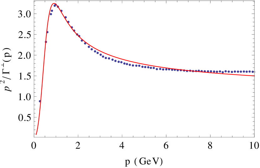
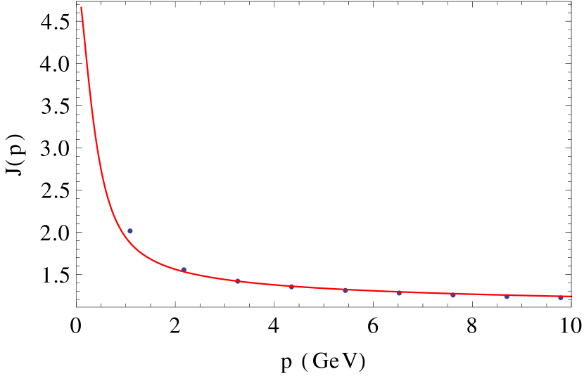
Figure 3: Gluon dressing function (top) and ghost dressing function (bottom) as a function of momentum in $d=4$ for $N_{f}=2$. The points are lattice data of Sternbeck:2012qs .

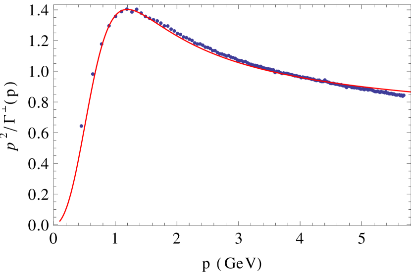
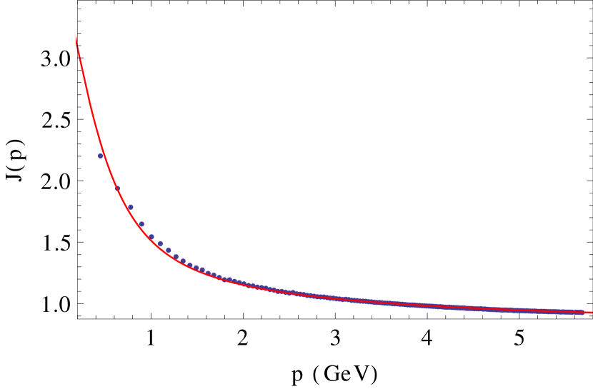
Figure 4: Gluon dressing function (top) and ghost dressing function (bottom) as a function of momentum in $d=4$ for $N_{f}=2+1+1$. The points are lattice data of Ayala:2012pb .

The contribution of the new diagram with an internal loop of quark is not strong enough to modify considerably the infrared behavior of the propagators due to the IR-safe structure of the quark propagator. Moreover the optimal values of the coupling constant and the gluon mass do not depend on slight changes in the quark mass. That means that the error for the gluon and ghost propagators do not change significantly if we change the value of the light quark mass slightly. Fig. 5 shows the contour regions for the errors. The contour regions are vertical, showing that the quality of the fit is almost insensitive to the quark mass (vertical axes).

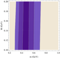
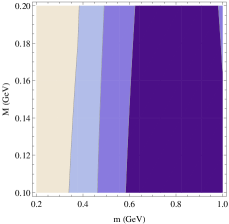
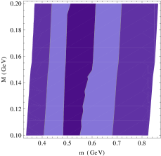
Figure 5: Contour levels for the quantities $\chi_{AA}$ (left) and $\chi_{c\bar{c}}$ (right) for $d=4$, both for $N_{f}=2$ (above) and $N_{f}=2+1+1$ (below). The contourlines correspond to 8%, 10% and 12 % (top left), 1.5%, 2% and 2.2 % (top right), 3%, 6% and 10 % (bottom left), 1%, 2% and 4% (bottom right).The quality of the fits is almost insensitive to the value of the quark mass.

As expected, if the quark mass considerably increases at values of the order of the GeV, the propagators tend to those obtained in the quenched approximation.

It is interesting to compare the results obtained for the gluon propagator and the ghost dressing function at one loop for different number of quarks. In Fig. 6 we present the gluon propagator and the ghost dressing function for $N_{f}=2$ and $N_{f}=2+1+1$. To compare their infrared behaviors, we normalized the curves such that they coincide at $4$ GeV. As was observed in lattice simulation Ayala:2012pb ; Bowman:2004jm , the addition of heavy quarks leads to a suppression of the IR saturation point . We also see that the ghost dressing function is enhanced.

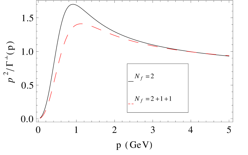
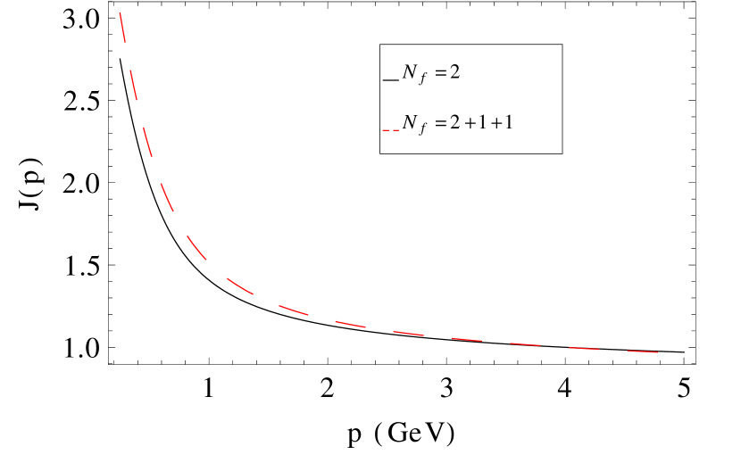
Figure 6: Gluon dressing function (top) and ghost dressing function (bottom) for different number of flavors in $d=4$

VI Results in the quark sector

We computed the quark propagator for arbitrary number of flavors but as the only available data for the quark sector corresponds to two degenerates light quarks plus a heavy one ($N_{f}=2+1$), we show the results only for this case. As in the previous section, we fixed the ratio of the light and heavy quarks to the ratio of the bare masses used in lattice simulations. Accordingly, in the present case, we fix the mass of the heavy quark to be five times heavier than the light one at $\mu_{0}=1$ GeV.

As discussed in the previous section, the fits of the gluon and ghost propagators are rather insensitive to the choice of the quark mass (see Fig. 5). However our results for $M_{u,d}(p)$ depend strongly on this parameter. Therefore we fixed the fitting parameters by minimizing simultaneously the error on the gluon propagator and on the function $M_{u,d}(p)$, $\chi_{M}$. (Note that the ghost propagator was not extracted from lattice simulations for $N_{f}=2+1$ and could not be used for fixing the parameters, see below.) It is defined as

$$\chi^{2}_{M}=\frac{1}{N}\sum_{i}M^{-2}_{\rm th.}(\mu_{0})\left(M_{\rm lt.}(p_{i})-M_{\rm th.}(p_{i})\right)^{2}$$ (7)

Note that we used a slightly different definition of the error. The reason is that the mass function becomes rapidly close to zero when the momentum grows. Accordingly a relative error point by point would be badly estimated because the signal to noise ratio of lattice data becomes of order one. In order to avoid this problem we normalized the data with a typical value of the mass in the infrared (at the scale $\mu_{0}$).

The best fit parameters are $g=4.8$, $m=0.42$ GeV and $M_{u,d}=0.08$ GeV at $\mu_{0}=1$ GeV. We insist on that the coupling and gluon mass are fixed from the gluon propagator and once this is done, we fixed the mass parameter from the scalar part of the quark propagator. The results obtained are shown in Fig. 7. The gluon propagator is again reproduced with an accuracy similar to that obtained for $N_{f}=2$ and $N_{f}=2+1+1$.

The one-loop results for $M_{u,d}(p)$ compare correctly with lattice simulations. In particular we retrieve the dramatic increase of the mass at a momentum scale of the order of 2 GeV. We want to stress that we could have a perfect fit of $M_{u,d}(p)$, but in doing so we would spoil the quality of the gluon propagator. Instead, we choose to maintain the quality of the gluon propagator at the prize of a not-so-good quark mass curve. In the Fig. 8 it is shown that there is a region of parameters where the fit is excellent (see Fig. 9), but we insist in using a value of the coupling compatible with a good fit for the gluon dressing function. The ghost dressing function was not extracted from lattice data and we can not test our findings in this case. However, we expect that this function is rather insensitive to the inclusion of a heavy quarks. Under this hypothesis, it is interesting to compare our findings with the ghost dressing function for $N_{f}=2+1+1$. We find fits (not shown) of the same quality as in the previous section.

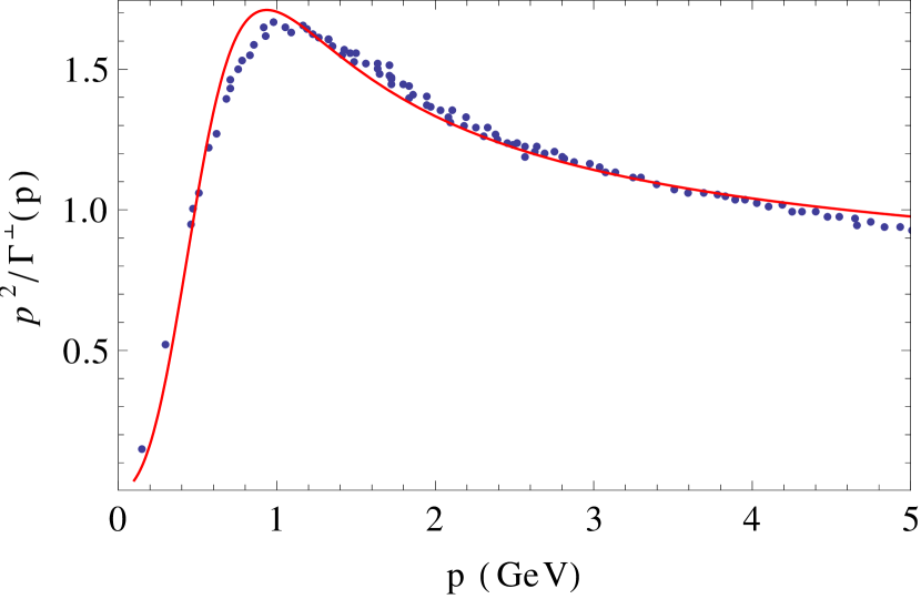
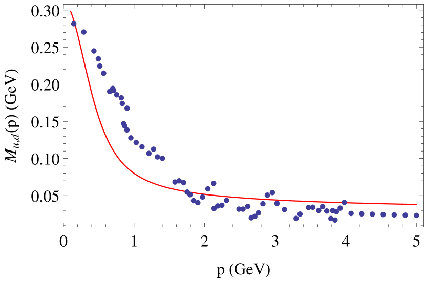
Figure 7: Gluon dressing function (top) and quark mass $M_{u,d}(p)$ (bottom) in $d=4$ for $N_{f}=2+1$. The parameters are $g=4.8$, $m=0.42$ GeV and $M=0.08$. The points are lattice data of Bowman:2004jm ; Bowman:2005vx .

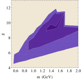
Figure 8: Contour levels for the quantity $\chi_{M}$. The contourlines correspond to 10%, 20% and 30 %.

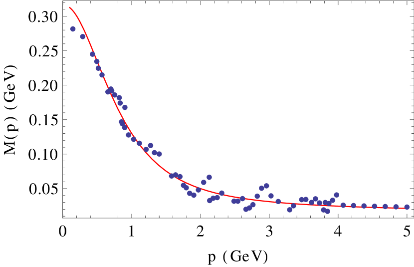
Figure 9: Quark mass $M_{u,d}(p)$ in $d=4$ for $N_{f}=2+1$. The parameters are $g=9.6$, $m=1.4$ GeV and $M=0.13$ GeV. The points are lattice data of Bowman:2004jm ; Bowman:2005vx .

For completeness, we also compare the mass functions for the light and heavy quarks in Fig. 10.

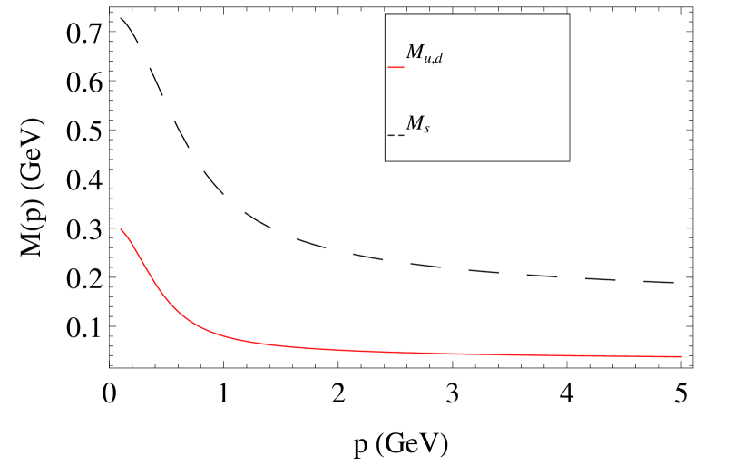
Figure 10: Quark masses of the light (full line, red) and heavy (dashed, black) quark.

If the one-loop correlation functions compare very well for the ghosts, gluons propagators and correctly for the function $M_{u,d}(p)$, the results for the quark renormalization function $Z_{u,d}(p)$ is not of the same quality , as can be seen in Fig. 11. We attribute this mismatch to the fact that the one-loop contribution to this function is unusually small. This is a consequence of the fact that, when the mass of the gluon is zero, $Z_{u,d}(p)$ has no contribution at one loop but it does have contributions at two-loops. In this situation, the two-loop contributions are not negligible and we do not expect a one-loop calculation to be sufficient for describing the characteristics of the field renormalization of the quarks. In the next section, we estimate the contribution of the two-loop diagrams and show that they have a small impact on our findings for the ghost and gluon propagators and on $M_{u,d}(p)$ but that they give a large contribution to $Z_{u,d}(p)$.

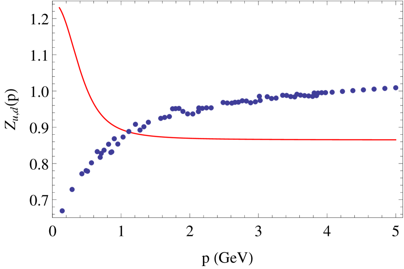
Figure 11: $Z_{u,d}(p)$ in $d=4$. The points are lattice data of Bowman:2005vx .

VII Preliminary estimate of two-loop contribution

The results presented in Fig. 11 show that first order perturbation theory is not enough to reproduce the behavior of the $Z(p)$ in the Landau gauge. For this reason we want to estimate the importance of two loop corrections. Ideally, we should compute all the two-loop diagrams and repeat the analysis performed above. Obviously this work exceeds the purpose of the present article.

Instead we use a cartoon expression of the two-loop $\beta$ functions (let us call it hybrid expression) obtained by complementing the $\beta$ functions and anomalous dimensions derived here at one loop with the ultraviolet two-loop contribution computed in Gracey:2002yt with a standard (massless) Faddeev-Popov Lagrangian. To take into account the suppression of massive contribution at low momenta, the ultraviolet two-loop contributions have to be appropriately regularized in that regime . Here we choose to modify the anomalous dimension presented in Gracey:2002yt in a minimal way by multiplying them by:

$$\frac{\mu^{2}}{\mu^{2}+s^{2}}$$

This factor goes to one in the UV limit where the whole expression matches with Gracey:2002yt . On the other hand, in the infrared regime it goes to zero as $\mu^{2}$, as expected. In the following, we present our results for $s=1$ GeV but we checked that we obtain the same conclusions by changing the parameter in the range 0.5—2 GeV.

We have performed a fit of the lattice data with this hybrid flow equations. The best fits were obtained for $g=3.4$, $m=0.4$ GeV and $M=0.08$ GeV, again defined at $\mu_{0}=1$ GeV. These fits are depicted in Fig. 13, in the center of the shaded areas. We estimate the error coming from neglecting the 2-loop contribution as the difference between the best fit in the hybrid model and in the purely one-loop calculation. In the Fig. 13 the hybrid calculation is taken as the central value (that includes a rough estimate of the two-loop contributions) and the error band estimated as explained just before is represented by the shaded area. We clearly see that higher corrections for the gluon propagator are small and compatible with the discrepancy between our one-loop results and the lattice data. The two-loop contribution to the function $M(p)$ is small but does not seem sufficient to make the one-loop results compatible with lattice data. This could be related with the spontaneous breaking of chiral symmetry which was not treated here. Finally, the corrections to $Z(p)$ are large and can explain the discrepancy between the lattice data and the 1-loop results. As mentioned in the previous section, this last function is therefore more difficult to describe and it is necessary to go to next to leading order to find a satisfactory matching.

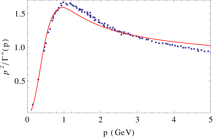
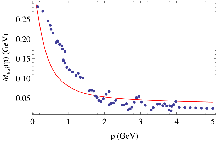
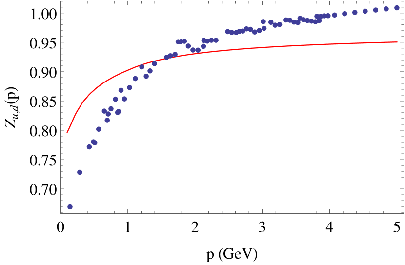
Figure 12: Gluon dressing function (top), quark mass $M(p)$(middle) and $Z(p)$ (bottom) in $d=4$ using the hybrid approximation. The points are lattice data of Bowman:2004jm ; Bowman:2005vx .

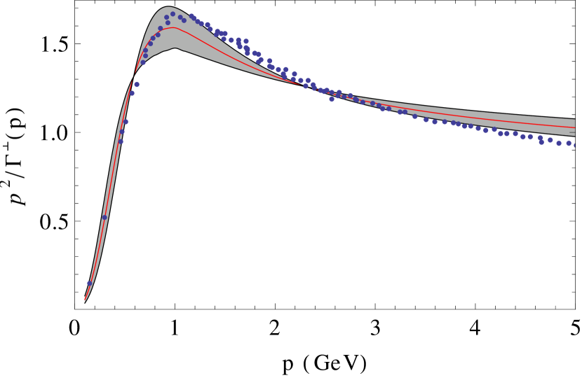
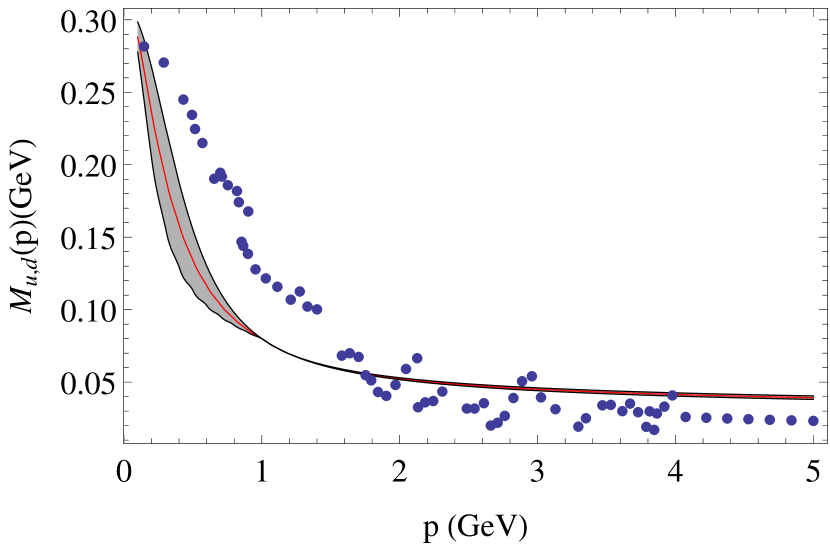
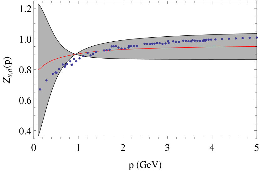
Figure 13: Gluon dressing function (top), quark mass $M_{u,d}(p)$ (middle) and $Z_{u,d}(p)$ (bottom) as a function of momentum in $d=4$. In red the hybrid calculation results (see text) and in black the one loop calculation and the symmetrized one loop results with respect to hybrid calculation. The points are lattice data of Sternbeck:2012qs and Bowman:2004jm ; Bowman:2005vx .

VIII Conclusions

In this article, we presented a one-loop calculation of the two-point correlation functions of QCD in the Landau gauge. The effect of the Gribov copies is minimally encoded in a mass term for the gluons. We find that the gluon and ghost propagators are reproduced with high precision. We estimate the higher order corrections to be small which seems to indicate that the Curci-Ferrari model reproduces well the lattice data.

On the other hand, one loop calculations are not enough to describe properly all the properties of the quark sector. The one loop contribution to $Z_{u,d}(p)$ function is very small and it vanishes if the gluon mass goes to zero in Landau gauge. That is why the two loops contributions are important and we have to take them into account if we want to quantitatively reproduce the $Z_{u,d}(p)$ function behavior.

The mass of the quark is correctly reproduced even though the accuracy is not as good as it is for the gluon sector. It is even unclear if a perfect matching for this quantity by such a simple one-loop calculation is possible given that we have not studied the influence of the chiral symmetry breaking. This analysis remains for a future work.

As we discuss in the article, computing the two loop contribution can help to estimate the validity of perturbation theory in this model. That is why we are considering in doing the two loop calculation completely.

- (1) V. N. Gribov, Nucl. Phys. B 139 (1978) 1.
- (2) D. Zwanziger, Nucl. Phys. B 323, 513 (1989).
- (3) D. Zwanziger, Nucl. Phys. B 399, 477 (1993).
- (4) D. Zwanziger, Phys. Rev. D 65 (2002) 094039.
- (5) D. Dudal, J. A. Gracey, S. P. Sorella, N. Vandersickel and H. Verschelde, Phys. Rev. D 78 (2008) 065047.
- (6) P. van Baal, Nucl. Phys. B 369, 259-275 (1992).
- (7) I. Montvay and G. Munster, “Quantum fields on a lattice,” Cambridge, UK: Univ. Pr. (1994).
- (8) A. Sternbeck, L. von Smekal, D. B. Leinweber and A. G. Williams, PoS LAT 2007, 340 (2007) [arXiv:0710.1982 [hep-lat]].
- (9) A. Cucchieri and T. Mendes, Phys. Rev. Lett. 100 (2008) 241601 and also arXiv:1001.2584 [hep-lat].
- (10) A. Cucchieri and T. Mendes, Phys. Rev. D 78 (2008) 094503.
- (11) A. Sternbeck and L. von Smekal, Eur. Phys. J. C 68, 487 (2010)
- (12) A. Cucchieri and T. Mendes, Phys. Rev. D 81 (2010) 016005.
- (13) I. L. Bogolubsky et al., Phys. Lett. B 676, 69 (2009).
- (14) D. Dudal, O. Oliveira and N. Vandersickel, Phys. Rev. D 81 (2010) 074505.
- (15) P. O. Bowman, U. Heller, D. Leinweber, M. Parappilly, A. Williams, and others, Phys. Rev. D 70, 034509 (2004).
- (16) M. B. Parappilly, P. O. Bowman, U. M. Heller, D. B. Leinweber, A. G. Williams and J. B. Zhang, AIP Conf. Proc. 842, 237 (2006) [hep-lat/0601010].
- (17) L. von Smekal, R. Alkofer and A. Hauck, Phys. Rev. Lett. 79 (1997) 3591.
- (18) R. Alkofer and L. von Smekal, Phys.Rept.353 (2001) 281.
- (19) C. S. Fischer and R. Alkofer, Phys. Rev. D 67 (2003) 094020.
- (20) J. C. R. Bloch, Few Body Syst. 33 (2003) 111.
- (21) C. S. Fischer, A. Maas and J. M. Pawlowski, Annals Phys. 324 (2009) 2408.
- (22) A. C. Aguilar and A. A. Natale, JHEP 0408 (2004) 057.
- (23) Ph. Boucaud et al., JHEP 06 (2006) 001.
- (24) A. C. Aguilar and J. Papavassiliou, Eur. Phys. J. A 35 (2008) 189.
- (25) A. C. Aguilar, D. Binosi and J. Papavassiliou, Phys. Rev. D 78 (2008) 025010.
- (26) P. Boucaud, J. P. Leroy, A. Le Yaouanc, J. Micheli, O. Pene and J. Rodriguez-Quintero, JHEP 06 (2008) 099.
- (27) J. Rodriguez-Quintero, JHEP 1101 (2011) 105.
- (28) M. Q. Huber and L. von Smekal, JHEP 04, 149 (2013) arXiv:1211.6092 [hep-th].
- (29) G. Curci and R. Ferrari, Nuovo Cim. A 32, 151 (1976).
- (30) J. Serreau and M. Tissier, Phys. Lett. B 712 (2012) 97 [arXiv:1202.3432 [hep-th]].
- (31) M. Tissier and N. Wschebor, Phys. Rev. D 82 (2010) 101701 [arXiv:1004.1607 [hep-ph]].
- (32) M. Tissier and N. Wschebor, Phys. Rev. D 84 (2011) 045018 [arXiv:1105.2475 [hep-th]].
- (33) M. Pelaez, M. Tissier and N. Wschebor, Phys. Rev. D 88, 125003 (2013).
- (34) B. Blossier, P. Boucaud, M. Brinet, F. De Soto, X. Du, M. Gravina, V. Morenas and O. Pene et al., Phys. Rev. D 85, 034503 (2012)
- (35) U. Reinosa, J. Serreau, M. Tissier, and N. Wschebor, Phys. Rev. D 89, 105016 (2014).
- (36) G. Passarino and M. J. G. Veltman, Model,” Nucl. Phys. B 160 (1979) 151.
- (37) A. I. Davydychev, P. Osland and O. V. Tarasov, Phys. Rev. D 54 4087 (1996).
- (38) A. I. Davydychev, P. Osland and L. Saks, Phys. Rev. D 63 014022 (2001).
- (39) J. A. Gracey, Phys. Lett. B 552, 101 (2003) [hep-th/0211144].
- (40) J. C. Taylor, Nucl. Phys. B 33 (1971) 436.
- (41) D. Dudal, H. Verschelde and S. P. Sorella, Phys. Lett. B 555 (2003) 126.
- (42) N. Wschebor, Int. J. Mod. Phys. A 23 (2008) 2961.
- (43) M. Tissier and N. Wschebor, Phys. Rev. D 79, 065008 (2009).
- (44) A. Sternbeck, K. Maltman, and M. Muller-Preussker and L. von Smekal , PoS LATTICE2012, 243 (2012).
- (45) A. Ayala, A. Bashir, D. Binosi, M. Cristoforetti and J. Rodriguez-Quintero, Phys. Rev. D 86, 74512 (2012).
- (46) P. O. Bowman, U. Heller, D. Leinweber, M. Parappilly, A. Williams, and others, Phys. Rev. D 71, 54507 (2005).