NGC 7538 : Multiwavelength Study of Stellar Cluster Regions associated with IRS 1–3 and IRS 9 sources.

Abstract

We present deep and high-resolution (FWHM $\sim$ 0$\aas@@fstack{\prime\prime}$4) near-infrared (NIR) imaging observations of the NGC 7538 IRS 1–3 region (in $JHK$ bands), and IRS 9 region (in $HK$ bands) using the 8.2 m Subaru telescope. The NIR analysis is complemented with GMRT low-frequency observations at 325, 610, and 1280 MHz, molecular line observations of H¹³CO⁺ ($J$=1–0), and archival Chandra X-ray observations. Using the ‘$J-H/H-K$’  diagram, 144 Class II and 24 Class I young stellar object (YSO) candidates are identified in the IRS 1–3 region. Further analysis using ‘$K/H-K$’  diagram yields 145 and 96 red sources in the IRS 1-3 and IRS 9 regions, respectively. A total of 27 sources are found to have X-ray counterparts. The YSO mass function (MF), constructed using a theoretical mass-luminosity relation, shows peaks at substellar ($\sim$0.08–0.18$~{}M_{\odot}$ ) and intermediate ($\sim$1–1.78$~{}M_{\odot}$ ) mass ranges for the IRS 1–3 region. The MF can be fitted by a power law in the low mass regime with a slope of $\Gamma\sim$ 0.54-0.75, which is much shallower than the Salpeter value of 1.35. An upper limit of 10.2 is obtained for the star to brown dwarf ratio in the IRS 1–3 region. GMRT maps show a compact H ii  region associated with the IRS 1–3 sources, whose spectral index of $0.87\pm 0.11$ suggests optical thickness. This compact region is resolved into three separate peaks in higher resolution 1280 MHz map, and the ‘East’  sub-peak coincides with the IRS 2 source. H¹³CO⁺ ($J$=1–0) emission reveals peaks in both IRS 1–3 and IRS 9 regions, none of which are coincident with visible nebular emission, suggesting the presence of dense cloud nearby. The virial masses are approximately of the order of 1000$~{}M_{\odot}$  and 500$~{}M_{\odot}$  for the clumps in IRS 1–3 and IRS 9 regions, respectively.

1 Introduction

NGC 7538, an optically visible H ii  region (Fich & Blitz, 1984, also known as Sh2-158), is a part of the Cas OB2 complex and located at $l=111.54^{o},~{}b=+00.78^{o}$, at a distance of 2.65 kpc (Moscadelli et al., 2009). Early infrared observations of this region by Wynn-Williams et al. (1974) and Werner et al. (1979) revealed the presence of infrared sources IRS 1-11 associated with and in the neighbourhood of the optical nebula. This region has been studied in prolific detail using various techniques such as high-frequency radio observations, line emission observations, maser observations, outflows, and so on. However, most of these studies as well as many recent ones concentrate on the individual features of luminous IRS and candidate high-mass sources. Even then, the bulk deals with the sources around IRS 1–3 stellar cluster region, and the IRS 9 region analyses have been sparse. Recently, an NIR study of the overall NGC 7538 region by Ojha et al. (2004a), reddening and cluster related studies using NIR by Balog et al. (2004), a spectroscopic study of the luminous sources by Puga et al. (2010), and a multiwavelength study of clusters (using statistical techniques) with a focus on high-mass stars by Chavarría et al. (2014) have been carried out. Other large scale studies have been carried out at far-infrared Herschel bands and at submillimetre wavelengths to identify cold clumps and filamentary structures (Sandell & Sievers, 2004; Fallscheer et al., 2013).

According to Ojha et al. (2004a) and McCaughrean et al. (1991), there appear to be three distinct sub-regions which can be separated based on the stellar population and morphology, namely the IRS 1–3, IRS 4–8, and IRS 9 sub-regions. Although the previous works identified a rich cluster membership in a wide ­field, encompassing all the major star-­forming sites in this complex, none of the optical/infrared surveys were deep enough to reach the substellar regime. Hence the works available in the literature were not able to have a detailed study of these stellar cluster sub-­regions, which need to be analysed separately due to their veritable differences. Recent advanced instruments on 8–10 m class telescopes now make it feasible to conduct imaging and spectroscopic studies of low-mass populations in distant high-mass star-forming regions, where the star-forming environment may be different from their low-mass counterparts. Moreover, in the case of stars in a distant cluster, high resolution imaging is also needed to recognize individual stars. Since most of the available studies of low-mass populations are mainly based on nearby star-forming regions and the sample of substellar sources is small to draw definitive conclusions, we considered it worthwhile to focus on the stellar clusters of the NGC 7538 region observed using the 8.2 m Subaru telescope - the deepest and highest-resolution NIR data till date. The NIR data has been used to study the luminosity function and initial mass function (IMF) of the region. In young massive star-forming regions, a gamut of components are present which could affect further evolution, and thus we have complemented our deep NIR observations with : previously unexamined low-frequency bremsstrahlung to ascertain the ionizing gas characteristics, molecular line H¹³CO⁺($J$=1 - 0) observations for the dense gas morphology, and Chandra X-ray observations for stellar population analysis.

In this paper, therefore, the aim is to continue with our multiwavelength study of star-forming regions (Ojha et al., 2004a, 2011; Samal et al., 2007, 2010), as well as our investigations to detect and characterize the young brown dwarfs (BDs) in distant massive star­-forming regions (cf. Ojha et al., 2004b, 2009). In Section 2, we present details of the observations and data reduction procedures. The YSO selection procedure is dealt with in Section 3. The spatial distribution, morphology, and physical characteristics of the regions are discussed in Section 4. In Section 5, we elaborate upon the luminosity and mass functions obtained for different clusters. Discussion and final conclusions are presented in Sections 6 and 7, respectively.

2 Observations and data reduction

2.1 Near Infrared Photometry

Deep NIR imaging observations of the NGC 7538 IRS 1-3 region (centered on $\alpha_{2000}=23^{h}13^{m}43^{s}$, $\delta_{2000}=$ +61^o28′ 22″) in $J$ ($\lambda=$1.25 $\mu$m), $H$ ($\lambda=$1.64 $\mu$m), and $K$ ($\lambda=$2.21 $\mu$m) bands, and the NGC 7538 IRS 9 region (centered on $\alpha_{2000}=23^{h}13^{m}58^{s}$, $\delta_{2000}=$ +61^o27′ 26″) in $H$ and $K$ bands were obtained on 2005 August 19, using the Cooled Infrared Spectrograph and Camera for OHS (CISCO) mounted at the Cassegrain focus of the 8.2 m Subaru telescope. These observations were done in the service mode of the telescope. CISCO is equipped with a 1024$\times$1024 Rockwell HgCdTe HAWAII array. A plate scale of 0.105″  pixel^-1 at the f/12 focus of the telescope provides a field-of-view (FoV) of $\sim$ 1.8′  $\times$ 1.8′  (Motohara et al., 2002). Observations were carried out in a 3$\times$3 dithering pattern with $\sim$ 10″  offsets - with a varying number of images (three upto ten) being obtained at each dithered position. Individual image exposure times were 40 s, 20 s, and 10 s for the $J$, $H$, and $K$ bands, respectively, finally yielding a total integration time of 12, 12, and 13.5 minutes in these respective bands. All the observations were done under excellent photometric sky conditions. The average seeing size was measured to be 0.4″  full-width-at-half-maxima (FWHM) in all three filters, and the air mass variation was between 1.34 and 1.44. Off-target (located $\sim$ 34′  east of the target position) sky-frame observations, identical in area to the target FoV, were taken just after the target observations using a similar procedure.

Data reduction was done using the Image Reduction and Analysis Facility (iraf) software package. The sky flats were generated by median-combining individual dithered sky frames for respective filters. These median-combined sky-flats were applied for both flat-fielding and sky subtraction. Identification of the point sources and their photometry was performed using the daofind and daophot packages of iraf. Because of source confusion and nebulosity within the region, photometry was performed using the point spread function (PSF) algorithm allstar in the daophot package (Stetson, 1987). An aperture radius of 4 pixels ($\sim$ 0.4″ ) was used for the final photometry, with appropriate aperture corrections applied for the respective bands. Since no standard star was observed during the observations, the photometric calibration was carried out using sources (about 10-12, cross-matched within 0.4″ of the Subaru catalogue) from the Two Micron All Sky Survey (2MASS), selected on the basis of their ‘phqual’  and ‘ccflg’  flag values, as well as visual examination, to avoid artifacts and contaminations. Finally, the photometric calibration rms was $\sim$ 0.1 mag. The Subaru/CISCO system magnitudes are assumed to be in California Institute of Technology (CIT) system (Oasa et al., 2006), and hence the 2MASS magnitudes too were converted to CIT system (using Carpenter, 2001) for calibration purpose. On comparison of our photometry with that of Ojha et al. (2004a), we find that the average dispersion (in the entire $K$ magnitude range) was $\sim$ 0.05-0.10 mag for the $JHK$ bands. Our higher spatial resolution permits better source separation and sky determination. Sources which were bright and saturated in Subaru images, but had good quality (‘phqual=A or B’  for $J$, $H$, and $K_{s}$ bands each) 2MASS photometry had their magnitudes taken from the 2MASS catalog after conversion to CIT system. Similar photometric procedure was also carried out for the off-target sky region. However, the western edge of the sky region was found to be slightly contaminated by a nearby nebula, and hence the sky frame was trimmed to remove the nebulous western portion before doing the photometry. The final sky frame size on which photometry (and completeness calculation below) was carried out is $\sim$ 1.17′ $\times$1.8′ . Since these observations were carried out in service mode, it was found that during the later observations, of IRS 9 region in $K$ band, source profiles at the north-east part of the images were elongated, due to some likely optics problem. Since this part (north-east of IRS 9 region) of the image is not crowded or nebulous, aperture photometry was carried out to estimate the source magnitudes of the sources with elongated profiles. Even then, due to limitations, we use IRS 9 photomtery for qualitative assessments only in this work.

The completeness limits of the images were evaluated through artificial star experiments using addstar in iraf. Since the IRS 1-3 and IRS 9 regions have varying nebulosity, the images were divided into separate regions as shown in Figure 1, followed by completeness determination for each sub-region. A fixed number of stars were added in every 0.5 magnitude interval, followed by photometry to see how many of these added stars were recovered. This cycle was carried out repeatedly. We thus obtained the detection rate - which is just the ratio of the number of recovered artificial stars to the number of added stars - as a function of magnitude for each of the sub-regions in IRS 1-3 and IRS 9 regions, as well as the sky region. Table 1 summarizes the 90% completeness limits for all three bands in each of the sub-regions. The 10$\sigma$ limiting magnitudes for our observations are estimated to be $\sim$ 22, 21 and 20 in the $J$, $H$, and $K$ bands, respectively. As can be seen, the sky frame 90% completeness limits are equal to these 10 $\sigma$ limiting magnitudes for the $H$ and $K$ bands, and slightly lower for the $J$ band.

2.2 Radio Continuum Observations

Radio continuum observations were carried out using the Giant Metrewave Radio Telescope (GMRT) for the frequency bands 325 MHz (2004 July 03), 610 MHz (2004 September 18), and 1280 MHz (2004 January 25). The GMRT array, consisting of 30 antennae, is in an approximate Y-shaped configuration. Each of these antennae has a diameter of 45 m, and thus a primary beam size of $\sim$ 81′ , 43′ , and 26.2′  for 325, 610, and 1280 MHz, respectively. There is a central region ($\sim$ 1 km$\times$1 km) which consists of randomly distributed 12 antennae, while the rest of the antennae are along three radial arms (6 along each arm) extending upto $\sim$ 14 km each. The minimum and maximum baselines are 100 m and 25 km, respectively. Further details about the GMRT array can be looked up in Swarup et al. (1991).

The total observation time ranged from $\sim$ 2.5-3.5 hours for the three frequency bands. Data reduction was carried out using the aips software. Successive rounds of flagging and calibration were carried out to improve the calibration. Flagging involved removal of bad data (including bad antennae, baselines, channels, time-ranges resulting from terrestrial radio frequency interference, etc), and was done using the ‘vplot-uvflg’  and ‘tvflg’  tasks. The respective flux and phase calibrators were used in the standard ‘calib-getjy-clcal’  procedure for amplitude and phase calibration. After satisfactory calibration, the source data (NGC 7538) was ‘split’  from the whole file (which contains flux and phase calibrator data in addition). Facet imaging was done using the aips task ‘imagr’  to generate the requisite images. To remove the ionospheric phase distortion effects, a few rounds of (phase) self-calibration - with decreasing ‘solint’  - were carried out using the task ‘calib’ . Table 2 gives the details of the GMRT observations and the parameters of the generated images. In addition, VLA archival image for 4860 MHz, for the observation date 2000 September 22 (Project ID BP0068), was also used in the analysis.

2.3 Chandra X-ray Observations

Publicly available archival X-ray data for NGC 7538 region was retrieved from the Chandra site (Obs. ID 5373). The X-ray observations of this H ii  region were carried out using the Advanced CCD Imaging Spectrometer (ACIS; Garmire et al., 2003) onboard the Chandra X-ray Observatory (CXO; Weisskopf et al., 2002). For our purpose, we use only the imaging array of ACIS (ACIS-I). ACIS-I consists of a 2$\times$2 CCD array of 1024$\times$1024 pixels each, with a total FoV of $\sim$ 17′$\times$17′ . The net exposure time was 30 ks.

Initial steps in the data reduction were carried out using the Chandra Interactive Analysis of Observations (ciao; Fruscione et al., 2006) tool version 4.5 and Chandra Calibration Database (caldb) version 4.5.8. The data was reprocessed using the ‘chandra_repro’  tool to apply the latest calibration to it. Light curve of source-free background regions were constructed to verify that the data was not affected by solar flare activity. Subsequently, with the help of the wavelet based source detection tool - ‘wavdetect’  (Freeman et al., 2002) - source detection was carried out at a threshold level of 2$\times$10^-6. Data image and exposure map with the default pixel scale of $\sim$ 0.5″  were used for this purpose. Once we have a final list of positions of detected sources from ‘wavdetect’ , we used the IDL based ACIS Extract (ae) software package (Broos et al., 2010, 2012) version ‘March 6, 2013’  to extract the relevant source properties. The algorithm detailed in the ae user’s guide was followed. The source counts are extracted within $\sim$ 0.90 PSF fraction, with the PSF being separate for each source. Within ae, the X-ray spectra are compiled and fitted with an optically-thin thermal plasma model attenuated by an interstellar absorption using the ‘xspec’  fitting package. A total of 182 sources were obtained in the FoV, all of which were verified to have P${}_{B}\leq$ 0.01, to make sure that the detected sources are real and not a result of Poissonian fluctuation in the local background. P_B gives the probability that the extracted counts in the total band are solely a result of background fluctuations. The intrinsic hard band luminosity for all the sources was found to range from $\sim$ 5.5$\times$10²⁸ to 3.5$\times$10³² erg s^-1, while the intrinsic total luminosity was in the range $\sim$ 5.5$\times$10²⁹ to 6$\times$10³⁵ erg s^-1. The hard band luminosity function peak was at about 5$\times$10³⁰ erg s^-1. For sources with spectral fitting results, the column density peaks at $\sim$ 10²² cm^-2 and the plasma temperature at $\sim$ 1 keV. The brightest ones show some metallic emission lines, supporting the thermal origin of the X-rays. These typical features are commonly seen among YSOs (Getman et al., 2006). We additionally used the non-parametric xphot program of Getman et al. (2010) to estimate the intrinsic fluxes and X-ray column densities.

Among the total number of sources obtained, there will also be extragalactic contaminants like Active Galactic Nuclei (AGN), and foreground stellar sources. Though we use a small subset of sources for our study (see Sections 3.1 and 3.2), and thus have not carried out a detailed contaminantion analysis here, we can obtain an estimate using the values for the Cepheus B region (Getman et al., 2006) which is close to NGC 7538 and had the same exposure time as well as FoV. Getman et al. (2006) find that the extragalactic contamination in Cepheus B is $\leq$ 5%, while stellar contamination is $\leq$ 4%. Assuming these numbers would imply a total of $\sim$ 16 contaminants (out of 182 total) in the NGC 7538 ACIS-I FoV. Table 3 gives the properties of 27 X-ray sources with NIR counterparts in the NIR FoV which have been selected in this paper for further analysis.

2.4 H¹³CO⁺($J$=1 - 0) Observations

The H¹³CO⁺ ($J$=1–0) (formylium) molecular line (86.754 GHz) observations were carried out on 2004 May 02 with the Nobeyama 45 m radio telescope. At 87 GHz, the half-power beam width and main beam efficiency, $\eta$, of the telescope were 18″ and 0.51, respectively. We used the 25-BEam Array Receiver System (BEARS) (Sunada et al., 2000). To correct for the beam-to-beam gain variation, we calibrated the intensity scale of each beam using a 100 GHz SIS receiver (S100) with an SSB filter. Furthermore, we observed the same grid point in mapping with 9 different beams to smooth the beam-to-beam gain variation. At the back end, we used 25 arrays of 1024 channel Auto-Correlators (ACs), which have a 32 MHz band width and a 37.8 kHz resolution, corresponding to 0.13 km s^-1 (Sorai et al., 2000). All the observations were carried out in position-switching mode. The standard chopper wheel method was used to convert the received intensity into the antenna temperature, $T_{\rm{A}}^{*}$. Our mapping observations covered the same region of the NIR image. The mapping grid has 21″  spacing, corresponding to half of the beam separation of the BEARS, i.e., nearly full-beam sampling. During the observations, the system noise temperatures were in the range of 200 to 400 K, resulting in a noise level of 0.35 K in $T_{{\rm A}}^{*}$. The telescope pointing was checked every 1.5 hours by observing the SiO maser source R Cas. The pointing accuracy was better than 3^′′.

3 YSO Selection

3.1 Using NIR Colour-Colour Diagram

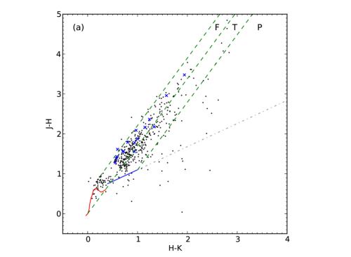
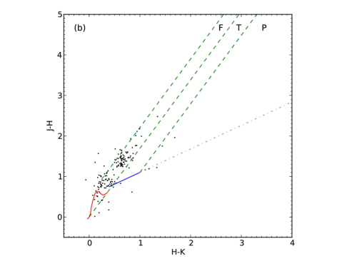
Figure 2: (a) $J-H/H-K$ NIR CC-D for the IRS 1-3 region. The red curve shows the dwarf locus from Bessell & Brett (1988). The CTTS locus (Meyer et al., 1997) is shown by the blue solid line, and its extension into the ‘P’  region by grey dot-dashed line. The three parallel and slanted dashed lines are the reddening vectors using the reddening laws of Cohen et al. (1981). Blue crosses mark the sources with X-ray counterparts. All points are in CIT system. (b) The CC-D for the sky field.

The photometric catalogs containing the $J$, $H$, and $K$ band magnitudes for the IRS 1-3 region (see Section 2.1) and the sky field region were used to construct the NIR J-H vs H-K colour-colour diagrams (CC-Ds) shown in Figure 2. In this figure, the red curve denotes the dwarf locus from Bessell & Brett (1988) (converted to CIT system), blue solid line denotes the locus of Classical T Tauri Stars (CTTS) from Meyer et al. (1997), and the three parallel dashed green lines denote the reddening vectors drawn using the reddening laws of Cohen et al. (1981) ($A_{J}/A_{V}=0.265,A_{H}/A_{V}=0.155,$ and $A_{K}/A_{V}=0.090$) for the CIT system. Three separate regions are marked on the images - ‘F’ , ‘T’ , and ‘P’  - similar to Ojha et al. (2004a, b). The ‘F’  region mostly contains the field stars and Class III-type (Weak-line T Tauri or WTTS) sources, the ‘T’  region mostly contains the CTTS and Class II-type sources (Lada & Adams, 1992), and the ‘P’  region mostly contains the Class I-type sources with circumstellar envelopes. Since the sources in the ‘P’  region can be contaminated by Herbig Ae-Be stars (Lada & Adams, 1992), we conservatively only consider those sources in this region whose J-H colour is larger than that of the CTTS locus extended into this region. There may also be an overlap in the NIR colours of the upper end band of Herbig Ae-Be stars and in the lower end band of CTTS in the ‘T’  region (Hillenbrand et al., 1992).

The sky field CC-D shown in Figure 2 is used to examine the extent upto which IRS 1-3 CC-D is affected by field star contamination. As can clearly be seen in Figure 2, almost all field star contamination is present in the ‘F’  region. Therefore, while the sources falling in the ‘T’  and ‘P’  regions of Figure 2 are most probably YSOs, the Class III-type sources from the ‘F’  region will be contaminated by field stars.

To further separate the most-likely YSOs from the ‘F’  region, since pre-main sequence (PMS) stars display much stronger X-ray emission than the field main sequence (MS) stars (Feigelson & Montmerle, 1999; Montmerle, 1996), we use the X-ray source identifications from Section 2.3. For this, we cross-matched our NIR catalog with the X-ray catalog within 0.5″ radius. X-ray detected sources, however, in general, suffer from extragalactic contamination (mostly AGN) and foreground stellar contamination. But since we are using only those X-ray sources which have NIR counterparts, it is unlikely - similar to the work of Getman et al. (2006, for Cepheus B) and Kuhn et al. (2010, for W40) - that there will be any extragalactic contamination. Also since the resolution of Chandra images ($\sim$ 0.5″ ) is similar to our NIR imaging ($\sim$ 0.4″ , see Section 2.1), mismatching should not be a concern. From the matching radius and the source number density, the number of X-ray sources to have an NIR counterpart by chance was calculated to be one at most. Apropos foreground contamination, the X-ray sources lie beyond the low-density gap at about $H-K\sim 0.5$ (again similar to Kuhn et al., 2010) in the NIR diagrams. Normally, a sudden low-density gap signifies the boundary of foreground sources in $H-K$ colour space. Hence, these X-ray matched sources are unlikely to be foreground contaminants too.

Finally - using the CC-D for IRS 1-3 region - 251 Class III-type sources including probable contaminants (14 have X-ray counterparts), 144 Class II-type sources (2 have X-ray counterparts), and 24 Class I-type YSO candidates were identified from the ‘F’ , ‘T’ , and ‘P’  regions, respectively. Table 4 lists these YSO candidates along with their respective NIR magnitudes, and IAU designation from Table 3 where applicable. Similar NIR CC-D could not be constructed for the IRS 9 region as we only have $H$ and $K$ magnitudes available for it.

3.2 Using NIR Colour-Magnitude Diagram

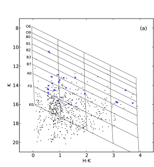
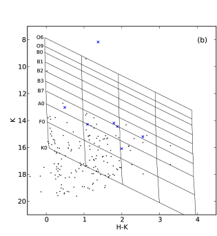
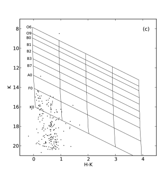
Figure 3: $K/H-K$ NIR CM-D for (a) IRS 1-3 region, (b) IRS 9 region, and (c) the sky region. Nearly vertical solid lines are the loci of ZAMS stars reddened by $A_{V}$=0, 15, 30, 45, and 60 mag. Parallel, slanting lines indicate the reddening vectors for respective spectral types. Blue crosses mark the sources with X-ray counterparts.

Many embedded and young sources can only be seen in $H$ and $K$ bands due to high extinction at $J$ band wavelengths. Therefore we use the K/H-K colour-magnitude diagram (CM-D) for the identification of additional YSOs. Figure 3 shows the K/H-K CM-D for IRS 1-3, IRS 9, and the sky field regions. The almost vertical solid lines represent the zero-age-main-sequence (ZAMS) locus at a distance of 2.65 kpc reddened by $A_{V}=$ 0, 15, 30, 45, and 60 mag. Slanting lines indicate the reddening vectors for the marked spectral types. A low density gap in $H-K$ colour $\sim 0.5$ can be seen in all three diagrams, though it is much less pronounced for the IRS 9 region due to the lack of statistics. In the sky field CM-D (Figure 3), we can see that most of the sources are confined to $H-K\leq 1$. This $H-K$(=1) limit also corresponds to the average extinction of $A_{V}=15$ mag found towards the NGC 7538 region by Ojha et al. (2004a). Thus, in general, a background contaminant field source suffering extinction due to the cloud should also be confined to $H-K\leq 1$. Also, on the same lines as Ojha et al. (2004a), if we were to assume that sources had large IR colours (say, $H-K>2$) purely due to interstellar extinction, then that would imply that the reddening due to molecular cloud is $A_{V}>$ 30 mag. But, with such a large $A_{V}$, diffuse emission will hardly be seen in NIR, which is definitely not the case here. Sources with colour over and above this limit (i.e. $H-K>1$) are therefore most likely to have large $H-K$ colour due to intrinsic infrared (IR) excess associated with YSOs. Hence, we use this colour cut-off of $H-K>1$ to identify extra YSO candidates from the IRS 1-3 and IRS 9 regions. To distinguish the YSO candidates identified using the NIR CM-D from those by the CC-D (Section 3.1), we refer to these sources as ‘red sources’  throughout the text. 145 sources (4 X-ray counterparts) were identified in the IRS 1-3 region, and 95 (7 X-ray sources with $H$ and $K$ counterparts $+$ 1 X-ray source with only $K$ counterpart) in the IRS 9 region. The catalogs of these red sources for the IRS 1-3 and IRS 9 regions are included in Tables 4 and 5, respectively.

4 Morphology and Spatial Distribution

4.1 IRS 1–3 region

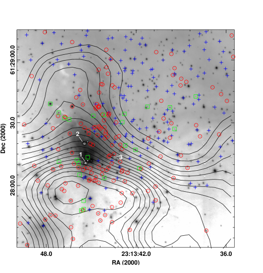
Figure 4: $K$ band image of the IRS 1-3 region overlaid with YSOs and H¹³CO⁺($J$=1–0) contours (black lines). The contours are drawn in the range 0.5–2.2 K km s^-1, with step size of 0.1 K km s^-1. Class I sources are shown with green square symbols, Class II with blue plus symbols, and sources with $H-K>1$ with red circles. IRS 1, 2, and 3 are saturated in the image and have been marked.

The $K$ band image of the IRS 1–3 region is shown in Figure 4 with the overlaid YSOs and H¹³CO⁺($J$=1–0) contours. Green squares mark the Class I sources, blue plus symbols the Class II-type or CTTS, and red circles the sources with $H-K>1$. IRS 1, 2, and 3 are saturated and have been marked. Dense cloud is seen around these marked IRS sources. There appears to be relatively higher nebulosity towards the northern as opposed to the southern region. Almost all stellar sources are present in the northern region. While the Class II-type sources (blue plus symbols) seem distributed throughout the northern part, sources with $H-K>1$ (red circles) and Class I sources (green squares) are mostly concentrated around the dense cloud surrounding the luminous IRS sources. Some of them could be PMS members of the embedded stellar clusters associated with the molecular clumps around IRS 1-3 and to the south of IRS 1-3. A few red sources are also seen around the ionization front (the boundary between darker nebulous region and the lighter non-nebulous region in the western part; see Section 4.3 too) at the interface between the H ii  region and the molecular cloud, which might have formed due to triggered star formation. The large diffuse emission extending to the north-west of IRS sources is probably due to a combination of free-free and bound-free emissions, corresponding to what is seen optically, and coincides well with the radio brightness from the GMRT observations, while the bright and compact infrared nebula embedded within IRS 1, 2, and 3 is coincident with the peak of radio continuum (see Section 4.3).

The H¹³CO⁺($J$=1–0) contours show a peak to the south-east of the IRS 1–3 nebula, where YSO density is much lower, and most of the sources around and near this peak are the red $H-K>1$ sources. Since this molecular emission traces the dense molecular cloud, it seems reasonable indeed that relatively very few sources are detected in the southern portion where the peak and the higher intensity contours lie, and the few sources detected are very reddened ones. The northern portion shows a hump in H¹³CO⁺($J$=1–0) contours, with contours closely spaced as one moves from the northern hump towards the southern peak. Preliminary calculations were carried out to get an idea of the column densities, local thermodynamic equilibrium (LTE) mass, and virial mass of the clump associated with the peak. Assuming LTE, we tried to estimate the molecular column density using the formula from Troitsky et al. (2005), with an excitation temperature of 10 K, and a dipole moment of 3.9 debye (Botschwina et al., 1993). Fitting a 2D Gaussian to the clump results in a peak integrated line intensity of 2.0 K km s^-1 and a source size at half intensity level of 1 pc. This gives us the LTE column density n(H¹³CO⁺) as $\sim 3.6\times 10^{12}$ cm^-2 after applying the main beam efficiency correction. Since the abundance - X(H¹³CO⁺) - estimates are variable from region to region and we do not have a measure of it here, we use the range seen for other massive star-forming regions - 0.5–3.0$\times$10^-10 from Zinchenko et al. (2009). Using these values, n(H₂) range is obtained to be $\sim$1.2–7.2$\times$10²² cm^-2, and the LTE mass range of the clump to be $\sim$250–1500$~{}M_{\odot}$ . The spectrum for the IRS 1–3 region clump is shown in Figure 5(upper). Applying a 1D fit to the spectrum of the clump, we obtain a linewidth of $\sim$ 3.4 km s^-1. The source size is corrected for the beam width to get the ‘deconvolved source size’  (Zinchenko, 1995). Using these values along with the expression from Zinchenko et al. (1994), the virial mass is approximated to be of the order of 1000$~{}M_{\odot}$ . Alternatively, under the reasonable assumption of gravitational equilibrium, the LTE mass and virial mass can be equated, which will imply an abundance X(H¹³CO⁺) of $\sim$ 0.74$\times$10^-10 - which is within the range derived by Zinchenko et al. (2009).

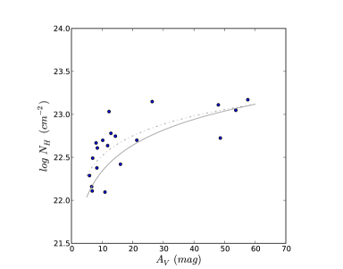
Figure 6: X-ray column density ($\log N_{H}$) vs visual extinction ($A_{V}$) plot for the sources in the IRS 1–3 region. The solid grey line marks the Ryter (1996) gas-to-dust relation of $N_{H}=2.2\times 10^{21}A_{V}$, while the dash-dotted grey line marks the relation from our analysis.

The gas-to-dust ratio for a cluster can be estimated by the relation obtained between the X-ray column density and the visual extinction for each source (Kuhn et al., 2010). Using the value of this column density ($logN_{H1}$) from Table 3 and $A_{V}$ from IR analysis (discussed in Section 5.1.2), we find $\log(N_{H}/A_{V})\sim 21.75\pm 0.20$. The relation is shown in Figure 6. It is slightly higher than that for the interstellar medium, $\sim$ 21.34 from Ryter (1996), and other young star-forming regions such as W40 (Kuhn et al., 2010). This higher value of gas-to-dust ratio is probably suggestive of dense gas in the region, as is also suggested by radio analysis (see Section 4.3).

4.1.1 Stellar Cluster Analysis

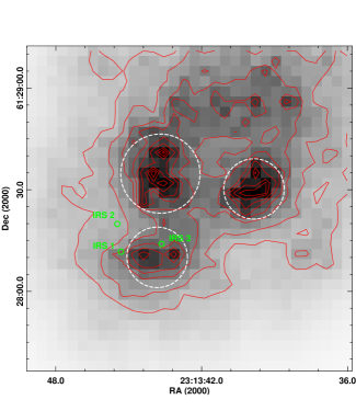
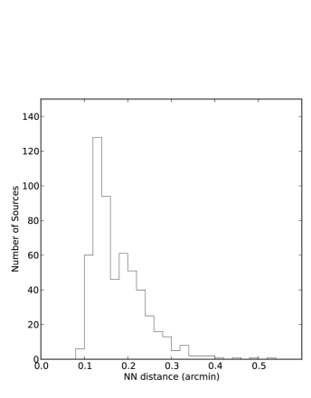
Figure 7: (left) 20 NN surface density map of the IRS 1-3 region with overplotted contours. The IRS sources have been marked by small green circles and labelled. The contour levels are at 250, 350, 500, 600, 700, 800, 900, 950, and 1000 YSOs pc^-2. Three distinct clusterings (indicated by white dashed circles) can be seen on the image - one close to the IRS 1 and IRS 3 sources, while the other two to the north and north-west of the IRS 3 source. All display multiple peaks. (right) The histogram of the NN distances of the sources.

A stellar surface density analysis of this region was carried out using the nearest-neighbour (NN) method (Casertano & Hut, 1985; Schmeja et al., 2008). We use the catalog of candidate YSOs identified in Section 3, and a procedure similar to Schmeja et al. (2008) with 20 NN. The resultant surface density map is shown in Figure 7(left), also overplotted with contours. Figure 7(right) shows the histogram of NN distances, with the peak NN distance in 0.12-0.14′  range. In Figure 7(left) three major clusterings can be made out. One is towards the south, associated with the IRS 1 and IRS 3 sources, while the other two are to the north and north-west of the IRS 3 source. Each of these clusterings display multiple peaks of their own. The maximum surface density values range from 860 to 1050 pc^-2, with the maximum exhibited by the clustering to the north of the IRS 3. These values are higher than the peak calculated for the overall NGC 7538 region by Chavarría et al. (2014), which could be a result of deeper data used here. These high peak values, though, are similar to that for Serpens Core(A) (1045 pc^-2; Schmeja et al., 2008).

4.2 IRS 9 region

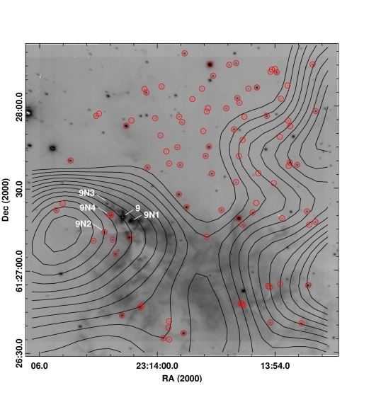
Figure 8: $K$ band image of the IRS 9 region overlaid with YSOs and H¹³CO⁺($J$=1–0) contours (black lines). The contours are drawn in the range 0.5–1.6 K km s^-1, with step size of 0.1 K km s^-1. Candidate YSOs have been shown with red circles. IRS 9, 9N1, 9N2, 9N3, and 9N4 sources from Ojha et al. (2004a) have been marked.

Figure 8 shows the $K$ band image of the IRS 9 region with the overlaid YSOs and H¹³CO⁺($J$=1–0) contours. Red circles denote YSO candidate sources. The main IRS sources - 9, 9N1, 9N2, 9N3, and 9N4 - from Ojha et al. (2004a) - have been marked on the image. As can be seen in Figure 8, sources are distributed throughout the image in no particular orientation, but with significantly more sources in the northern portion as opposed to the nebular southern portion - possibly an indication of the high extinction in this nebular region. This suggests that the region is extremely young, also affirmed by the fact that there is no free-free radio emission seen in the nebulous part (see Section 4.3). There appears to be clustered star formation going on around the IRS 9 region. The IRS 9N4 source from Ojha et al. (2004a) is resolved into two distinct sources in this image. The H¹³CO⁺($J$=1 - 0) molecular line emission peak lies to the eastern portion of the IRS 9 sources, a region deficient in YSOs. This indicates the presence of dense gas in this region. A 450 $\mu$m clump from Reid & Wilson (2005) is close to this peak. Using the same procedure as for the IRS 1–3 region (see Section 4.1), a peak integrated line intensity of 1.5 K km s^-1, and a source size at half intensity level of $\sim$ 0.77 pc, LTE column density n(H¹³CO⁺) is calculated to be $\sim 2.7\times 10^{12}$ cm^-2. This leads to n(H₂) range of $\sim$ 0.9–5.4$\times$10²² cm^-2, and an LTE clump mass range of $\sim$ 100–660$~{}M_{\odot}$ . The spectrum for the clump is shown in Figure 5(lower). The virial mass - following same steps as for IRS 1–3 region - is approximately of the order of 500$~{}M_{\odot}$ . Alternatively, as Section 4.1, assuming gravitational equilibrium gives X(H¹³CO⁺) $\sim$ 0.65$\times$10^-10.

4.3 Radio Continuum Emission

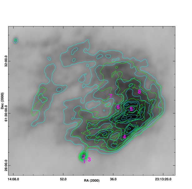
Figure 9: The maximum resolution radio continuum images for 325 MHz (cyan contours; 12.3″ $\times$ 8.7″ ) and 610 MHz (green contours; 9.0″ $\times$ 4.6″ ) obtained using GMRT for the entire NGC 7538 region. The contours for 325 MHz image are drawn at 12, 17, 25, 30, 35, 37, 40, and 42 $\sigma$ ($\sigma\sim$ 1.78 mJy). 610 MHz contours are drawn at 2.5, 5, 7, 10, 15, and 20 $\sigma$ ($\sigma\sim$ 4 mJy). The IRS sources in this FoV are marked by their respective numbers in magenta. The background image is 325 MHz radio image.

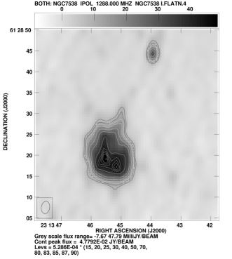
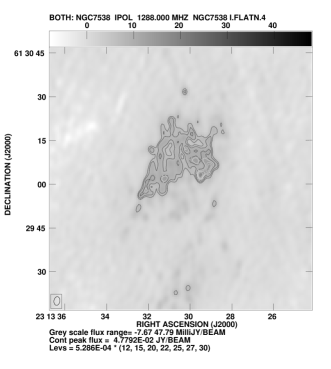
Figure 10: The maximum resolution radio continuum images for 1280 MHz (3″ $\times$2″ ). (left) IRS 1-3 region. Three separate cores are resolved here - to the North, East, and West. The contours are at 15, 20, 25, 30, 40, 50, 70, 80, 83, 85, 87, and 90 $\sigma$ ($\sigma\sim$ 0.53 mJy). (right) High resolution image of the north-west part of the NGC 7538 region, around the source marked ‘5’  in Figure 9. The contours are drawn at 12, 15, 20, 22, 25, 27, and 30 $\sigma$ ($\sigma\sim$ 0.53 mJy).

The maximum resolution radio continuum images of the entire NGC 7538 region which could be constructed are shown for 325 MHz (resolution $\sim$ 12.3″ $\times$ 8.7″ ), 610 MHz (resolution $\sim$ 9.0″ $\times$ 4.6″ ), and 1280 MHz (resolution $\sim$ 3″ $\times$ 2″ ) (Figures 9 and 10). The positions of the IRS sources in the region have been indicated by numbers in Figure 9. The radio contours in Figure 9 show a definite champagne flow morphology (Tenorio-Tagle, 1979; Whitworth, 1979). While the contours are closely packed in the south-west corner, they become spread as one moves from the south-west to the north-east direction. The south-west corner is density bounded, while the north-east side is ionization bounded. In the relatively lower resolution 325 and 610 MHz maps (Figure 9), there are definite peaks associated with IRS 1-3, as well as with the other IRS sources 4 and 5 (note that these IRS 4 and 5 sources are outside our NIR FoV). The peak around the IRS 1-3 region is resolved into three separate peaks - to the North, East, and West - in the higher resolution 1280 MHz image (Figure 10(left)). Out of these, the IRS 1-3-East peak coincides with the IRS 2 source. As can be seen in this high-resolution image, the corresponding radio source for IRS 2 has a cometary appearence, as has also been observed at higher radio frequencies (Bloomer et al., 1998; Campbell & Persson, 1988). The IRS 1-3-North and West peaks do not have any NIR sources associated with them, though the IRS 1-3-West peak (keeping in mind that the beam size is $\sim$ 3″ $\times$ 2″  here) is very close to the IRS 2C peak from the 6 cm radio map of Campbell & Persson (1988). The IRS 1-3-East and West cores are approximately of the size of the synthesized beam ($\sim$3″ $\times$2″ ), with a flux of $\sim$ 50 mJy and 30 mJy, respectively. The IRS 1-3-North core is $\sim$3.8″ $\times$2.3″  in size, with a total flux of $\sim$43.4 mJy. Based on the size of the cores (Kurtz & Franco, 2002), the whole IRS 1-3 core can be classified as a compact H ii  region (size from 0.1 to 0.5 pc), while the North, East, and West cores can be classified as ultracompact H ii  regions (size $\la$ 0.1 pc). The high resolution 1280 MHz image near the north-west part of the NGC 7538 region (near the sources marked 4 and 5 in Figure 9; outside our NIR FoV) also shows multiple cores (Figure 10(right)).

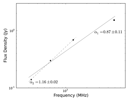
Figure 11: SED fitting for the IRS 1-3 compact H ii  region. The circular markers show the data points from the GMRT at 325, 610, and 1280 MHz, while the square marker shows the VLA data point at 4860 MHz. The solid grey line is the fitting using all four data points (with spectral index $\alpha_{1}=$0.87$\pm$0.11), and the dashed grey line shows the fit using only the GMRT points (with spectral index $\alpha_{2}=$1.16$\pm$0.02).

The nature of a free-free emission region can be studied by calculating its spectral index $\alpha$, given by $S_{\nu}\propto\nu^{\alpha}$, where $\nu$ is the frequency and $S_{\nu}$ is the integrated flux density of the region at $\nu$. We can calculate the spectral index using $d\log S_{\nu}/d\log\nu$. As free-free emission changes from optically thick to optically thin, $\alpha$ varies from 2 to -0.1 (Panagia & Felli, 1975; Olnon, 1975). First of all, we obtained all the GMRT images at the same uniform resolution of about $\sim$12″ $\times$9″  (as this is the maximum resolution map we could make for 325 MHz). Next, we calculated the integrated flux density within the IRS 1-3 compact H ii  region for all three frequencies. In addition to the GMRT frequencies, VLA archival image at the frequency of 4860 MHz (at a very similar resolution of $\sim$14.9″ $\times$11.5″ ) was also obtained and integrated flux density calculated for the compact H ii  region. The values obtained are given in Table 2. Figure 11 shows the radio SED fit using these data points. The solid grey line shows the SED fit using all four data points ($\alpha_{1}=0.87\pm 0.11$), while the dashed grey line shows the fitting ($\alpha_{2}=1.16\pm 0.02$) using only the GMRT points. These values of $\alpha$ suggest that the region is optically thick at these low frequencies, in consistency with earlier radio studies (Akabane et al., 1992).

If we assume that this compact H ii  region is homogeneous and spherically symmetric, then we can calculate the Lyman continuum photon luminosity (photon s^-1) using the following formula from Moran (1983, see their Equation 5) :

$$S_{*}=8\times 10^{43}\left(\frac{S_{\nu}}{mJy}\right)\left(\frac{T_{e}}{10^{4}K}\right)^{-0.45}\left(\frac{D}{kpc}\right)^{2}\left(\frac{\nu}{GHz}\right)^{0.1}$$ (1)

where $S_{\nu}$ is the integrated flux density in mJy from the contour map, $D$ is the distance in kiloparsec, $T_{e}$ is the electron temperature, and $\nu$ is the frequency in GHz for which the luminosity is to be calculated. Now choosing the VLA data point of 4.860 GHz (as it will lie in the most optically thin regime of the free-free emission SED), and $T_{e}$ a typical value of 10000 K (Panagia & Felli, 1975; Olnon, 1975), $S_{*}$ was calculated to be $\sim$ 1.01$\times$10⁴⁸ (i.e. $\log S_{*}\sim 48.00$). According to the tabulated values of Panagia (1973), this much flux would correspond to a ZAMS O9 star ($\log S_{*}=48.08$). Using various techniques, the spectral types of IRS 1, 2, and 3 in the literature have been found to be consistent with O6 ZAMS (Willner, 1976; Pestalozzi et al., 2004) (though Franco-Hernández & Rodríguez (2004) give O8.5), O9.5 ZAMS (Campbell & Thompson, 1984; Bloomer et al., 1998), and a B-type star (Puga et al., 2010), respectively. However, various analyses have found extremely high extinction towards the IRS 1 source. Willner (1976) has concluded that the optical depth associated with IRS 1 is high enough to absorb 99% of UV photons. Similarly large extinction properties have been found by Campbell & Persson (1988) and Beuther et al. (2012) in their study of this source. Hence, if we exclude IRS 1, then our Lyman continuum luminosity is consistent with that for a O9.5 ZAMS source (IRS 3 contribution, being a B-type source, will be much lesser comparatively). This high extinction could be the reason why IRS 1 source is not seen in our high resolution 1280 MHz map in Figure 10(left). Additionally, this caveat of dust absorption of radiation suggests that O9 ZAMS spectral type should be the lower limit and the actual spectral type could be earlier than this.

5 Luminosity and Mass functions

We use the YSO catalogs from Section 3 to generate the $K$-band luminosity function (KLF) of the IRS 1-3 and IRS 9 stellar clusters. $K$ band, as opposed to $H$ or $J$ band, is used as : the effects of extinction are minimum, it probes sources upto much fainter luminosities, and the results can be compared to the existing literature.

5.1 IRS 1-3 region

5.1.1 $K-$band luminosity function

KLFs for the IRS 1-3 region were generated using 2 sets of YSOs taken from Table 4 : the first set containing a combination of ‘F+T+P+red-sources’  (basically the entire Table 4), and a second set containing only ‘T+P+Any source with X-ray detection’  (see Section 3 and Figures 2 and 3). This was done as the first set may contain YSO candidates with field star contamination and will need to be corrected for it, while the second set is most likely YSOs with much lower field contamination. To derive the KLF of a region, one needs to apply corrections for the following : star count incompleteness (which is a function of magnitude), and the field star contamination towards the cluster.

Star count incompleteness was corrected for by using the completeness calculations from Section 2.1. The completeness fraction had been obtained for each 0.5 magnitude bin. The counts in each magnitude bin were scaled up by dividing the counts by the completeness fraction in the respective bins. This gives us the completeness-corrected KLF.

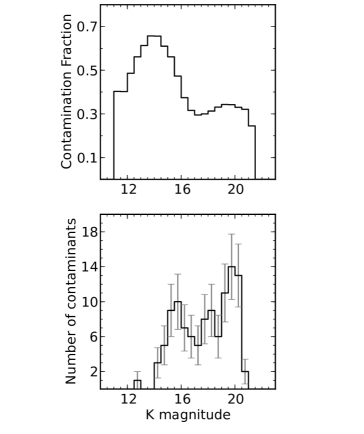
Figure 12: (upper) The contamination fraction (per magnitude bin) calculated using the Galactic model of Robin et al. (2003). (lower) The number of contaminants (per magnitude bin) for the IRS 1-3 cluster region. The error bars show the error due to counting statistics. A similar exercise was carried out for the IRS 9 region.

The field star contamination was assessed using the sky field source catalog (from Section 2.1) in conjunction with the Galactic model of Robin et al. (2003), similar to Ojha et al. (2004a, b). Two sets of catalogs were generated using the Besançon model of stellar population synthesis (Robin et al., 2003) in the direction of the sky field region. The first set contains the sources generated by setting $A_{V}=4.4$ mag, which was chosen as it is the average $A_{V}$ of sources in the sky field CM-D (between $H-K=0$ and the low density gap at $H-K=0.5$), and thus most likely to be the foreground extinction of sources towards this region. From this first catalog set, we get the total number of sources as well as the number of foreground sources in the direction of the sky field region. The foreground sources, in this catalog, are simply the ones with distances $<2.65$ kpc. In addition to the total and foreground sources towards this region, we need to assess the background field star contamination too. However, the background field star contaminants will suffer an extra extinction due to the intervening molecular cloud, which needs to be taken into account. Now, the average extinction towards the NGC 7538 region has been found to be $A_{V}=15$ mag (Ojha et al., 2004a). If we assume a spherical geometry of the molecular cloud medium, then it follows that the sources behind the molecular cloud should suffer an extinction of $A_{V}=15+15=30$ mag. Therefore, we generated a second model catalog set by setting $A_{V}=30$ mag. In this second set, all the sources with distances $>2.65$ kpc will give us the background contaminants. After having obtained the total, foreground, and the background sources, the $K$ band histogram (with binwidth$=$0.5) was plotted and the contamination fraction (foreground+background/total) was obtained for each bin. Finally, to obtain the absolute number of contaminating sources in each magnitude bin, we use the sky field $K$ band histogram. Each magnitude bin of the sky field $K$ magnitude histogram is scaled by the ratio ($\sim 0.75$) of the areas of sky field to IRS 1-3 region, as well as by its contamination fraction calculated above. Fig. 12 shows the contamination fraction, along with the number of field contaminants in the IRS 1-3 region, as a function of magnitude. The obtained contaminant number in each bin was subtracted from the completeness-corrected KLF (binwise) to obtain the field- and completeness-corrected KLF.

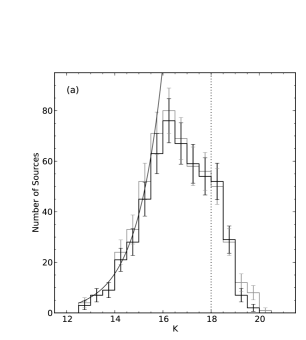
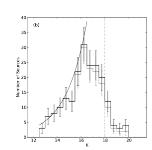
Figure 13: KLFs for the IRS 1-3 region. (a) For ‘F+T+P+red-sources’  sources. Grey line histogram represents the raw KLF. Solid black line histogram shows the final field- and completeness-corrected KLF. (b) For ‘T+P+Any source with X-ray detection’  sources. Grey line is for the raw KLF, while the black line shows the final completeness-corrected KLF. The vertical dotted line in both figures marks the $K$ band 90% completeness limit at 18 mag. The error in each bin is the Poissonian $\pm\sqrt{N}$ error. The black curve shows the power law fit to the KLF.

The KLFs for the first YSO set (‘F+T+P+red-sources’ ), and second YSO set (‘T+P+Any source with X-ray detection’ ) are shown in Figure 13. A binsize of 0.5 has been chosen as it is much larger than the errors in source magnitudes. To compare with the literature, we calculate the $(d\log N/dm_{K})$ slope for the rising part of the KLFs to be $0.40\pm 0.03$ (in the magnitude range 12.5–16.5) for the first YSO set, and $0.24\pm 0.03$ (in the magnitude range 12.5–16.5) for the second YSO set. While the KLF slope for the first YSO set is higher than that for the completeness- and field-corrected KLF for the whole NGC 7538 region ($0.30\pm 0.03$) from Ojha et al. (2004a), it is similar to that of the NGC 1893 ($\sim$ 3.25 kpc; $0.34\pm 0.07$) from Sharma et al. (2007), Tr 14 ($\sim$ 2.5 kpc; $0.37\pm 0.01$) from Sanchawala et al. (2007), and IRAS 06055+2039 ($\sim$ 2.6 kpc; $0.43\pm 0.09$) (Tej et al., 2006). The slope for the second set is consistent with that calculated earlier in Ojha et al. (2004a) for the completeness-corrected whole NGC 7538 region ($0.28\pm 0.02$) as well as that for the younger regions in NGC 7538 ($0.27\pm 0.03$). It is also very close to the value for the whole W3 region ($\sim$ 1.83 kpc; $0.26\pm 0.01$) (Ojha et al., 2004b) and Sh2-255 IR region ($\sim$ 2.6 kpc; $0.17\pm 0.03$) from Ojha et al. (2011). A turnoff is seen in both the KLFs after 16-16.5 magnitude bin, similar to the Tr 14 region from Sanchawala et al. (2007).

5.1.2 Mass Function

The mass function (MF) is usually described by the following differential form :

$$\xi(\log\,M_{*})=dN/d\log M_{*}$$ (2)

where $N$ is the number of stars and $M_{*}$ is mass of stars (Bastian et al., 2010; D’Antona, 1998; Chabrier, 2003; Kroupa et al., 2013). Since magnitude ($m_{K}$), and not mass ($M_{*}$), is an observable quantity, $\xi$ has to be re-written as :

$$\xi(\log\,M_{*})=dN/d\log M_{*}=(dN/dm_{K})\div(d\log M_{*}/dm_{K})$$ (3)

where $(dN/dm_{K})$ is nothing but the KLF slope, and $(d\log M_{*}/dm_{K})$ represents the derivative of the so-called mass-luminosity relation (MLR). If we have the form of the KLF and the MLR derivative, then $\xi$ can be evaluated.

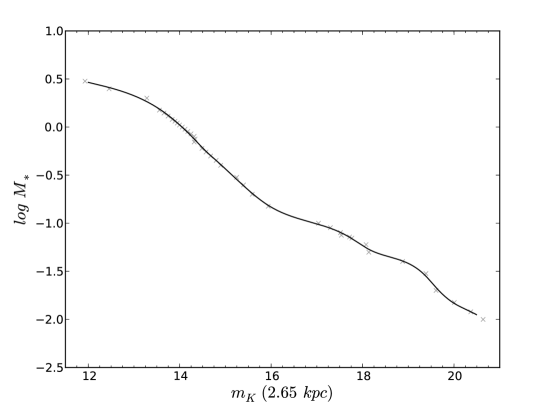
Figure 14: (upper) MLR from literature (see text). The grey crosses mark the data points from literature and the black line shows the fitted curve to it. We confine our analysis to $m_{K}\geq 12$, i.e. lower limit of MLR.

The MLR depends on the age of the cluster, and in our case we use the age estimate of 1 Myr for the NGC 7538 region from Ojha et al. (2004a). The theoretical isochrones (for 1 Myr) from Baraffe et al. (2003) (for the mass range $0.01-0.1$ M_⊙), Baraffe et al. (1998) ($0.15-1.50$ M_⊙), and Palla & Stahler (1999) ($2.0-3.0$ M_⊙) are used for the MLR. The absolute magnitudes were converted to apparent magnitudes using the distance modulus (at a distance of 2.65 kpc). The complete MLR is shown in Figure 14, along with the curve fit to it. To calculate $\xi$, we need the derivative of this MLR. We limit our analysis to sources with $m_{K}\geq 12$ mag, as it the lower limit of the MLR.

In addition to the MLR, a form of the intrinsic KLF is also needed. To derive the intrinsic KLF, the sources were corrected for extinction by dereddening them along the reddening vectors to the respective loci as per the following order of steps. First, the sources which were present in the ‘F’  region of the NIR CC-D (Figure 2) were dereddened to the dwarf locus (whose low-mass regime - from the turn-over onwards - was approximated by a straight line; similar to Tej et al., 2006; Samal et al., 2007), while those in the ‘T’  and ‘P’  regions were dereddened to the CTTS locus. The rest of the sources (those not dereddened using the NIR CC-D) were dereddened using the $H$ and $K$ magnitudes to the ZAMS locus (approximated by a straight line) in the NIR CM-D (Figure 3) to estimate their extinctions, though this is only an approximation as the YSOs are most-likely not on ZAMS yet. The major source of uncertainty in using the CM-D is the correction of the locus for distance, which need not be well-determined. The individual visual extinction of the sources was found to range upto 60 mag. This is much deeper, as expected, than upto 40 mag which was estimated by Ojha et al. (2004a) for their detected YSOs. The histogram (not shown here) of these visual extinctions was found to peak in the range 7.5-10 mag. The mean extinction value was $\sim$ 15 mag, consistent with that used for model simulations in Section 5.1.1 and Ojha et al. (2004a). The sources with $A_{V}>40$ mag were mostly found to be distributed along the southern boundary between the nebulous and non-nebulous region (also see Figs. 1(left) and 4). A few such sources were also associated with the small nebular patch at the south-east corner of the IRS 1-3 region.

Using this catalog of reddening-corrected sources, field-, completeness-, and reddening-corrected KLFs were obtained for the two YSO sets (‘F+T+P+red-sources’  being the first set and ‘T+P+Any source with X-ray detection’  being the second set; see Section 5.1.1). To preserve the information about the form of the KLF, different magnitude intervals (each interval containing three or more bins) were fit with equations of straight line using simple linear regression. This gives us the KLF slope for each magnitude bin.

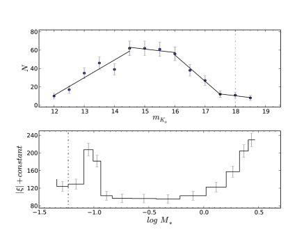
Figure 15: KLF fits and $\xi$ (differential form) for ‘F+T+P+red-sources’  YSO catalog in the IRS 1-3 region. (upper) The field-, completeness-, and reddening-corrected KLF and the straight line fits to its different portions. (lower) $\xi$ calculated using equation 3. Each 0.5 mag bin from the KLF has been mapped to a corresponding bin in $\log M_{*}$ space here. The vertical dashed-dotted line indicates the 90% completeness limit. Poissonian errors are marked for each bin.

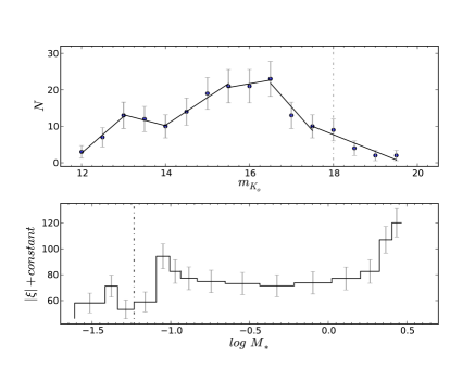
Figure 16: KLF fits and $\xi$ for ‘T+P+Any source with X-ray detection’  YSO catalog in the IRS 1-3 region. Rest is same as for Figure 15.

After we obtain the KLF slope $(dN/dm_{K})$ in each magnitude bin and the form of the MLR derivative ($d\log M_{*}/dm_{K}$ at discrete points), value of $\xi$ is calculated using Equation 3 for each magntiude bin - which is further mapped onto the $\log M_{*}$ space using the MLR. The resulting form of $\xi$ is shown in Figures 15 and 16 along with the KLFs. Poissonian error of $\pm\sqrt{N}$ is marked for each bin. It should be kept in mind that equal magnitude intervals do not map onto equal $\log M_{*}$ intervals. The shape of the $\xi$ is closest to that derived by Scalo (1986) for field stars, with a peak at the low mass end, and another peak at the intermediate mass (Meyer et al., 2000). The low mass peak is at $\log M_{*}$ bin of $-1.09$ to $-1.00$, i.e $0.08-0.1\,M_{\odot}$ (for Figures 15 and 16). This rise in the MF till the BD limit has been seen for other regions like W3 Main (Ojha et al., 2009) and S106 (Oasa et al., 2006) too, as well as mentioned likely by Kroupa (2007). The curve does not extend enough in the intermediate mass range to clearly discern the peak.

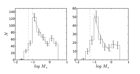
Figure 17: IRS 1-3 region : $N(\log M_{*})$ for (left) ‘F+T+P+red-sources’  YSO catalog, and (right) ‘T+P+Any source with X-ray detection’  YSO catalog obtained by assigning mass to each source individually and binning. Error bars in each bin show Poissonian error. The grey curve shows the fit to the MF in 0.1–1 M_⊙ mass range. The vertical dashed line indicates the mass corresponding to the $K$ 90% completeness limit of 18 mag. The binwidth is 0.25.

Another way to test the MF form is to use the MLR to assign a mass to each star in the catalog, and then bin those masses to obtain the $N(\log M_{*})$, rather than the differential form $\xi(\log M_{*})$ (Chabrier, 2003, see its Section 1.3). Using this, we obtain the MFs shown in Figure 17. The field star subtraction for the first catalog here was carried out statistically using the NIR CM-D as follows. Similar to Sharma et al. (2007), we divided the CM-Ds of the IRS 1-3 region and the sky field region into grids with $\Delta K$=0.5 mag and $\Delta(H-K)$=0.1 mag. The number of stars was compared on a grid-by-grid basis, and from the IRS 1-3 CM-D, a fixed number of stars (equal to the number in the corresponding sky field grid) was removed based on their distances to the sky field stars in the colour-magnitude space. Each grid was corrected for incompleteness.

As can be seen, the MFs are similar in shape to those in Figures 15 and 16, with a peak in the $\log M_{*}=$ -0.75 – -1.0 bin (i.e. 0.1–0.18 M_⊙), and another at $\log M_{*}=$ 0–0.25 bin (i.e. 1–1.78 M_⊙). However, the peak at the lower mass regime, though consistent with the other method, is on the slightly higher side here. The mass range of the turn-off point in the lower mass regime is consistent with those for other prominent clusters in the literature (Bastian et al., 2010), like $\sigma$ Orionis (Peña Ramírez et al., 2012), $\rho$ Ophiuchi (Alves de Oliveira et al., 2012), IC 348 (Alves de Oliveira et al., 2013), and Orion Nebula Cluster (Hillenbrand & Carpenter, 2000). A secondary peak seen here is also observed in the IMF of the $\rho$ Ophiuchi cluster from Alves de Oliveira et al. (2012) and Orion Nebula Cluster from Hillenbrand & Carpenter (2000). If we assume a power law form of the MF (similar to Salpeter, 1955), then :

$$dN/d(\log M_{*}) \propto M_{*}^{-\Gamma}$$ (4)

$$\Rightarrow dN/dM_{*} \propto M_{*}^{-(\Gamma+1)}.$$ (5)

Now, if we additionally assume that the star formation is strictly coeval, then it can be mathematically shown that

$$-\Gamma=d(\log N)/d(\log M_{*}),$$ (6)

and that the present day mass function will have the same slope as the IMF (Massey, 1998, see its Section 2.1). Also, since the age of this region is $\sim$ 1 Myr, which is lower than the MS life of even the most massive stars, none of the stars would have disappeared from the field. In Figure 17, fitting the sub-solar low mass range (between the first and the second peaks, i.e. 0.1-1 M_⊙) using Equation 6, we get the value of $\Gamma$ for the first and second YSO sets as $0.54\pm 0.05$ (say, $\Gamma_{1}$) and $0.75\pm 0.18$ (say, $\Gamma_{2}$), respectively. Both the slopes are lower than the Salpeter slope of 1.35. While $\Gamma_{1}$ seems consistent with that from Kroupa (2002) (also see Figure 2 of review by Bastian et al. 2010), $\Gamma_{2}$ is slightly steeper. This steepness, though, might be explained by the fact that Figure 17(right) includes mostly the youngest sources with fainter magnitudes - thus making this MF ‘bottom-heavy’ , i.e. more sources at lower mass ranges. On the other hand, Figure 17(left) includes Class III sources and thus more sources in relatively higher mass ranges. In general, more complicated/realistic forms of the IMF can emerge due to accretion processes, leading to a tail towards the high mass end (Dib et al., 2010), which will become noticeable only in high-mass star-forming regions where the intermediate to high-mass bins are well populated. Finally, we should keep in mind the caveat that any derivation of an IMF suffers from multiple unavoidable and systematic biases, e.g. those arising due to - among others - choice of the stellar MLR, PMS evolution, effect of unresolved sources, binning, etc. Kroupa et al. (2013, see their Section 2.1) have dealt with these biases in a succinct manner. Different treatment of these biases might accordingly alter a derived IMF.

The ratio of stars to BDs in a region is often used as another quantitative indicator for the mass function. We consider the following two definitions of this ratio :

$$R_{1} = N(0.08<M/M_{\odot}\leq 1)/N(0.03\leq M/M_{\odot}\leq 0.08),and$$ (7)

$$R_{2} = N(0.08<M/M_{\odot}\leq 10)/N(0.02\leq M/M_{\odot}\leq 0.08),$$ (8)

similar to Scholz et al. (2012). However, since our observations are complete only upto 0.06 M_⊙, the R₁ and R₂ values obtained will be the upper limit. Taking this caveat into account and using the above equations, we get the value of $R_{1}<349/44\sim 8$, and $R_{2}<470/46\sim 10.2$. The compilation by Scholz et al. (2012) shows that the values of $R_{1}$ and $R_{2}$ for other star-forming regions lie in the range 2–8, while Luhman et al. (2007) state that $R_{2}$ ranges from 5–8 in star-forming regions. On the other hand, Alves de Oliveira et al. (2012) find higher value of $R_{2}$ (upto 11 depending on their analysis parameters) in the $\rho$ Ophiuchi cluster. However, given the fact that the values of $R_{1}$ and $R_{2}$ calculated here are upper limits, they are consistent with those of other star-forming regions.

5.2 IRS 9 region

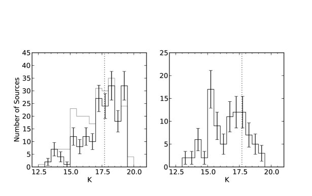
Figure 18: KLFs for the IRS 9 region. (left) The grey line histogram shows the raw KLF of all sources detected in $K$-band, while the black line shows the KLF after field- and completeness-correction. (right) KLF of sources which had $H-K>1$, or were detected in X-ray. Error bars are Poissonian. The vertical dotted line marks the $K$ band 90% completeness limit at 17.7 mag.

We obtained the KLF for the IRS 9 region using the catalog of sources identified in at least $K$ band, as well as the catalog of candidate YSOs (red sources with $H-K>1$ identified in Section 3.2 and those with X-ray emission). The KLFs are shown in Figure 18. Figure 18(left) shows the raw KLF (grey line) along with the field- and completeness-corrected KLF (black line). Since the statistics are low for this region, we only make a few qualitative comparisons here. The $(d\log N/dm_{K})$ slope was calculated to be $0.20\pm 0.04$ (in 13–19 $K$ mag range), and is lower than that calculated for younger regions in Ojha et al. (2004a) and some other star-forming regions (see Section 5.1.1), though similar to Sh2-255 IR region (Ojha et al., 2011). The KLF of red sources ($H-K>1$) is shown in Figure 18(right). There appear to be two peaks in Figure 18(right) - one near 15–15.5 mag and another at about the completeness limit (marked by a dotted vertical line). The KLF seems to be plateauing near the completeness limit. The brighter peak is most likely to be due to field contamination, which has not been corrected for due to a lack of statistics here. If we consider the 16–17.7 mag interval of this YSOs’ KLF, we see that it first has a steeper slope in the 16–16.5 mag interval, and then plateaus off in the 16.5–17.7 mag interval. This steep slope followed by plateauing is seen in other regions like NGC 1624 (Jose et al., 2011) and Sh2-255 IR region (Ojha et al., 2011) too, albeit for different magnitude limits. In this range (16–17.5), the slope comes out to be $0.24\pm 0.11$, which is very similar to that from Ojha et al. (2004a) for younger regions of NGC 7538, and is consistent within errors with that obtained for the Sh2-255 IR region (Ojha et al., 2011).

6 Discussion

Analysis of star-forming regions in different stages is essential in understanding how star formation proceeds and the effect of manifold physical processes on various diagnostic tools (like LF, MF, etc). In general, however, physical conditions (like density, temperature, chemical composition) could differ from one region to another. The study of NGC 7538 cluster regions (IRS 4-6, IRS 1-3, and IRS 9, which follow an age sequence in descending order; Ojha et al., 2004a), being part of the same complex, should mitigate this problem. Here, using the deepest NIR data, we have obtained the KLF and the MF of the IRS 1-3 region, while only the KLF of the IRS 9 region has been discussed. The MF for the IRS 1-3 region shows that it rises till the BD limit before turning over, which indicates lower temperature or denser gas distribution than for Orion nebula cluster (Hillenbrand & Carpenter, 2000; Muench et al., 2002), though comparison of LF and MF of different regions from literature always follow the caveat that the method used for their construction might be slightly different. Presence of dense molecular material has been attested by surveys in submillimetre ranges too (Sandell & Sievers, 2004; Reid & Wilson, 2005). Our molecular line analysis also reveals massive clumps which could fragment and lead to future stellar cluster formation. The 850 $\mu$m emission (Chavarría et al., 2014) shows the IRS 1-3 region to be located on a junction of filaments, which could partially explain the active star formation going on. Confinement of most IR clusters at filament junctions has also been observed by Schneider et al. (2012) and obtained in the simulations of Dale, Ercolano, & Bonnell (2012). The entire morphology of NGC 7538 seems similar to the hub-filament structure proposed by Myers (2009), where the IRS 1-3 cluster region forms the ‘hub’  to which various filaments merge. The molecular hydrogen column density (which is $>10^{23}\,cm^{-3}$; Fallscheer et al., 2013) satisfies the condition which Myers (2009) proposes for a ‘hub’ .

The IRS 9 region, however, appears to be distinct and at one end of the filament which connects it with IRS 1-3 (this filament goes on to connect IRS 4 too; see Sandell & Sievers, 2004). IRS 9 region has been found to be much younger than IRS 1-3, owing to a lack of free-free radio emission as well as a low number of YSOs associated with the nebula. The Herschel temperature maps (Fallscheer et al., 2013) also show that IRS 9 is much colder than IRS 1-3 region. The decreasing age-sequence along the filament connecting the three cluster regions of IRS 4-6, IRS 1-3, and IRS 9 alludes to the possibility that star formation could have been triggered along this filamentary structure.

To gain a firm understanding of the NGC 7538 region stellar population, as well as the evolution of the KLF and MF as one moves from relatively older to relatively younger regions in a star-forming region, we need to obtain the detailed LFs and MFs for the IRS 4-6 region as well as IRS 9 region. The advantage will be that all the sub-regions belong to the same region NGC 7538, and should therefore differences arising due to the differences in physical conditions (leading to different temperature and density distributions, which leads to different Jeans masses and thus different LFs/MFs) need not be a concern. Future analysis of the BDs detected in the region, construction of MF from a spectroscopic sample, an analysis of core mass function of this region, and examination of spectral energy distributions of individual sources are also required for a better idea of the star formation going on.

7 Conclusions

We have carried out the deep NIR imaging survey of IRS 1–3 ($J,H$, and $K$) and IRS 9 ($H$ and $K$) sub-regions in the NGC 7538 star-forming region with the highest spatial resolution so far. In addition, GMRT observations at 325, 610, and 1280 MHz are used to examine the radio emission and physical characteristics. H¹³CO⁺ ($J$=1–0) molecular line emission from Nobeyama radio telescope is used to understand the morphology. Our main results are summarized as follows.

1. Based on the NIR CC-D ($J-H/H-K$), 144 Class II-type, and 24 Class I-type YSOs were identified in the IRS 1–3 region. Using the NIR CM-D ($K/H-K$), 145 sources were identified in the IRS 1-3 region, and 96 in IRS 9 region. 27 sources were found to have X-ray counterparts.

2. In the IRS 1–3 region, the red sources and the Class I sources are concentrated around the compact nebula associated with luminous IRS sources, and the H¹³CO⁺ ($J$=1–0) contours show a peak (column density n(H¹³CO⁺) $\sim 3.6\times 10^{12}$ cm^-2) to the south of these sources. Stellar surface density analysis reveals three clusterings in this region. The IRS 9 region does not have any particular distribution of the YSOs, with the nebula hardly containing any sources. An H¹³CO⁺ ($J$=1–0) peak (n(H¹³CO⁺) $\sim 2.7\times 10^{12}$ cm^-2) lies to the east of the cluster around IRS 9 source. The virial masses are approximately of the order of 1000$~{}M_{\odot}$  and 500$~{}M_{\odot}$  for the clumps in IRS 1–3 and IRS 9 regions, respectively.

3. Radio emission shows a champagne flow morphology in the NGC 7538 region. In low-resolution 325 and 610 MHz maps, a compact H ii  region is seen associated with IRS 1–3 sources, with its spectral index calculated to be $0.87\pm 0.11$, suggesting optically thickness. In very high resolution 1280 MHz maps, the IRS 1–3 compact H ii  region is resolved into three separate peaks, one of which coincides with the known IRS 2 source.

4. KLFs were constructed for IRS 1–3 region for two sets of sources : ‘F+T+P+red-sources’  and ‘T+P+Any source with X-ray detection’ . The rising part of the KLF has a $(d\log N/dm_{K})$ slope of $0.40\pm 0.03$ for the first set, and $0.24\pm 0.03$ for the second set ($K$ magnitude range 12.5–16.5). The KLF slopes for the IRS 9 region using sources with $K$ band only detections was calculated to be $0.23\pm 0.04$ (13–19 mag).

5. Theoretical mass-luminosity relation is used to obtain $\xi(\log M_{*})$ (differential form of MF) and $N(\log M_{*})$ for the IRS 1–3 cluster region. Both $\xi(\log M_{*})$ and $N(\log M_{*})$ show a peak in the low mass regime as well as a peak in the intermediate mass regime. In low-mass regime, $\xi(\log M_{*})$ extends upto BD limit before turn-off (0.08–0.1 M_⊙), while $N(\log M_{*})$ peak is in 0.1–0.18 M_⊙ range. The slope $d\log N/d\log M_{*}$ (from $N(\log M_{*})$ distribution) for the first and second YSO sets in the range 0.1–1 M_⊙ are $0.54\pm 0.05$ and $0.75\pm 0.18$, respectively - much lower than the Salpeter value of 1.35. The MFs most closely resemble that of Scalo (1986). The star to BD ratio upper limit was calculated to be 10.2.

Table 1: 90% Completeness Limits for NIR bands

	$K$	$H$	$J$
	(mag)	(mag)	(mag)
IRS 1-3 region
Overall	18	19	20.2
1	17	18.4	19.2
2	18.5	19.4	20.2
3	18	20	19.7
IRS 9 region
Overall	17.7	16.6
1	19.2	16.6
2	17.7	16.6
Sky region
Whole	20	21	21.2

Table 2: Details of Radio Continuum Observations

	1280 MHz	610 MHz	325 MHz	VLA 4860 MHz Archival Image
Date of Obs.	2004 January 25	2004 September 18	2004 July 03	2000 September 22 (BP0068)
Phase Center	$\alpha_{2000}$ = 23h13m44s	$\alpha_{2000}$ = 23h13m45.28s	$\alpha_{2000}$ = 23h13m45.28s
	$\delta_{2000}$ = 61o28${}^{{}^{\prime}}$44.24${}^{{}^{\prime\prime}}$	$\delta_{2000}$ = 61o28${}^{{}^{\prime}}$09.07${}^{{}^{\prime\prime}}$	$\delta_{2000}$ = 61o28${}^{{}^{\prime}}$09.07${}^{{}^{\prime\prime}}$
Flux Calibrator	3C48	3C48	3C48, 3C147
Phase Calibrator	2355+498	2350+646	2350+646
Cont. Bandwidth	16 MHz	16 MHz	16 MHz
Primary Beam	26.2${}^{{}^{\prime}}$	43${}^{{}^{\prime}}$	81${}^{{}^{\prime}}$
Resolution of maps
used for fitting	11.5${}^{{}^{\prime\prime}}\times$ 8.5${}^{{}^{\prime\prime}}$	12.0${}^{{}^{\prime\prime}}\times$ 8.1${}^{{}^{\prime\prime}}$	12.3${}^{{}^{\prime\prime}}\times$ 8.7${}^{{}^{\prime\prime}}$	14.9${}^{{}^{\prime\prime}}\times$ 11.5${}^{{}^{\prime\prime}}$
rms noise	1.93 mJy beam-1	6.82 mJy beam-1	1.78 mJy beam-1	1.56 mJy beam-1
Integrated flux density
for IRS 1-3 region	0.69 Jy	0.30 Jy	0.14 Jy	1.53 Jy

Table 3: X-ray Sources with NIR counterparts in the NIR FoV

Source					Xspec (Using ACIS Extract)						Xphot
IAU Designation	RA	Dec	$C_{t,net}$	$E_{median}$	log NH1	kT1	log Lh1	log Lt1	log Lhc1	log Ltc1	log Lhc2	log Ltc2	log NH2
	(deg)	(deg)	(counts)	(keV)	(cm-2)	(keV)	(erg s-1)	(erg s-1)	(erg s-1)	(erg s-1)	(erg s-1)	(erg s-1)	(cm-2)
(1)	(2)	(3)	(4)	(5)	(6)	(7)	(8)	(9)	(10)	(11)	(12)	(13)	(14)
231336.03$+$612806.5	348.400166	61.468476	14.9	2.2	22.491	1.751	30.703	30.783	30.848	31.331	30.761	31.195	22.176
231338.51$+$612847.0	348.410483	61.47973	4.9	3.	22.096	9.528	30.299	30.364	30.336	30.519
231338.72$+$612836.9	348.41136	61.476943	8.9	2.5	22.699	1.591	30.581	30.627	30.815	31.348	30.802	31.063	22.301
231339.47$+$612832.8	348.41448	61.475793	32.9	2.6	22.609	2.023	31.157	31.205	31.329	31.756	31.296	31.662	22.342
231339.94$+$612756.8	348.416427	61.465791	5.9	4.1	22.78	5.005	30.623	30.635	30.791	31.028	31.044	31.499	23.041
231340.28$+$612902.2	348.417839	61.483949	6.9	1.9	22.288	1.749	30.249	30.379	30.343	30.826
231340.65$+$612847.0	348.419397	61.479739	6.9	2.3	22.109	6.095	30.443	30.517	30.483	30.699	30.429	30.924	22.23
231340.78$+$612828.1	348.419949	61.474477	28.9	2.8	22.668	2.015	31.134	31.172	31.326	31.754	31.33	31.655	22.398
231341.96$+$612742.6	348.424864	61.46184	15.9	3.5	22.7	8.762	31.058	31.071	31.187	31.375	31.225	31.649	22.708
231342.29$+$612830.5	348.426229	61.475165	5.8	3.5	23.033	2.268	30.585	30.59	30.941	31.331	30.864	31.216	22.716
231342.71$+$612848.7	348.427984	61.480202	4.9	3.1	22.16	9.526	30.349	30.406	30.39	30.574
231343.97$+$612807.4	348.43321	61.468723	30.7	4.3	23.111	8.697	31.476	31.477	31.745	31.933	31.862	32.216	23.079
231344.26$+$612809.8	348.434439	61.469415	11.7	3.8	22.377	9.528	30.771	30.807	30.837	31.021	31.254	31.659	22.875
231345.02$+$612842.5	348.437602	61.478481	4.8	4.	22.637	9.52	30.487	30.503	30.598	30.782
231345.05$+$612807.8	348.437735	61.46886	15.7	3.9	22.725	9.528	30.993	31.004	31.123	31.308	31.415	31.779	22.886
231345.35$+$612807.9	348.438981	61.468886	25.7	4.	23.048	3.574	31.321	31.322	31.62	31.905	31.666	32.023	22.924
231345.41$+$612825.4	348.439217	61.473744	35.8	4.	22.747	7.085	31.424	31.436	31.57	31.773	31.762	32.172	22.947
231346.32$+$612752.8	348.443014	61.464692	4.8	3.8	23.171	1.908	30.542	30.544	31.032	31.48
231347.06$+$612819.8	348.446089	61.472175	3.8	3.7	23.149	2.275	30.47	30.471	30.899	31.286
231348.88$+$612822.6	348.453703	61.47296	6.9	3.7	22.42	9.528	30.977	31.011	31.052	31.234	31.332	31.737	22.778
231352.30$+$612654.6	348.467923	61.448523	4.9	1.9	22.921	0.543	30.452	30.555	31.035	32.634
231357.29$+$612815.5	348.488749	61.470973	5.9	5.	22.655	9.528	30.618	30.633	30.734	30.918	31.543	31.979	23.477
231358.62$+$612819.3	348.494256	61.472035	5.9	3.7	22.583	9.528	30.585	30.605	30.686	30.869	30.915	31.315	22.785
231400.86$+$612646.9	348.503605	61.446368	8.9	2.4	21.238	9.528	30.367	30.512	30.373	30.556	30.622	31.084	22.301
231401.57$+$612752.9	348.506575	61.464702	87.9	2.5	22.4	4.23	31.775	31.823	31.856	32.115	31.841	32.173	22.255
231401.78$+$612643.6	348.507435	61.445464	8.9	3.2	23.184	1.265	30.743	30.747	31.381	32.064	30.97	31.307	22.591
231402.39$+$612720.1	348.509978	61.455607	6.9	3.6	22.411	9.528	30.611	30.644	30.681	30.865	30.955	31.389	22.771

Col. (1–3): IAU designation, RA and Dec. Col. (4–5): Net counts extracted in the total energy band (0.5–8 keV); Background-corrected median photon energy (total band). Col. (6–7): Column density and plasma temperature calculated using Xspec. Col. (8–9): Apparent hard and total band luminosity Col. (10–11): Intrinsic hard and total band luminosity Col. (12–14): Intrinsic hard band luminosity, total band luminosity, and the column density calculated using Xphot.

Table 4: YSOs in IRS 1-3 NIR FoV

RA	Dec.	$J$	$H$	$K$	YSO Classification,
(J2000)	(J2000)	(mag)	(mag)	(mag)	X-ray IAU Designation
348.438812	61.461308	21.014 $\pm$ 0.024	17.398 $\pm$ 0.001	15.335 $\pm$ 0.034	ClassIII
348.438904	61.486595	19.365 $\pm$ 0.023	18.038 $\pm$ 0.010	17.004 $\pm$ 0.015	ClassII
348.438995	61.468994		17.973 $\pm$ 0.010	14.514 $\pm$ 0.026	$H-K>1$,231345.35$+$612807.9
348.439117	61.467808	20.258 $\pm$ 0.030	15.619 $\pm$ 0.010	12.824 $\pm$ 0.095	ClassII
348.439117	61.473797	16.536 $\pm$ 0.034	14.370 $\pm$ 0.020	13.220 $\pm$ 0.023	ClassIII,231345.41$+$612825.4

The IAU designation is from Table 3. Table 4 is available in its entirety in a machine-readable form in the online journal. A portion is shown here for guidance regarding its form and content.

Table 5: YSOs in IRS 9 NIR FoV

RA	Dec.	$H$	$K$	X-ray IAU Designation
(J2000)	(J2000)	(mag)	(mag)
348.46637	61.466164	16.278 $\pm$ 0.012	15.167 $\pm$ 0.005
348.466431	61.454922	18.088 $\pm$ 0.022	15.91 $\pm$ 0.009
348.46701	61.470901	17.93 $\pm$ 0.013	16.225 $\pm$ 0.013
348.467743	61.454628	19.445 $\pm$ 0.03	17.492 $\pm$ 0.017
348.467987	61.448483	15.983 $\pm$ 0.009	14.191 $\pm$ 0.004	231352.30$+$612654.6

The IAU designation is from Table 3. Table 5 is available in its entirety in a machine-readable form in the online journal. A portion is shown here for guidance regarding its form and content.

Figure 1: (left) Colour composite image of the IRS 1-3 region using $J$ (blue), $H$ (green), and $K$ (red) bands. Three sub-regions are marked on the image using cyan rectangles. (right) Colour composite image of the IRS 9 region using $H$ (green), and $K$ (red) bands, with two sub-regions marked. Each sub-region of the respective region has been labelled by a number. Completeness limit was calculated for each sub-region.

Figure 5: The H¹³CO⁺($J$=1–0) molecular line spectra towards (upper) the peak in IRS 1–3 region, and (lower) the peak in IRS 9 region.

References

- Akabane et al. (1992) Akabane, K., Tsunekawa, S., Inoue, M., et al. 1992, PASJ, 44, 421
- Alves de Oliveira et al. (2012) Alves de Oliveira, C., Moraux, E., Bouvier, J., & Bouy, H. 2012, A&A, 539, A151
- Alves de Oliveira et al. (2013) Alves de Oliveira, C., Moraux, E., Bouvier, J., et al. 2013, A&A, 549, A123
- Balog et al. (2004) Balog, Z., Kenyon, S. J., Lada, E. A., et al. 2004, AJ, 128, 2942
- Baraffe et al. (1998) Baraffe, I., Chabrier, G., Allard, F., & Hauschildt, P. H. 1998, A&A, 337, 403
- Baraffe et al. (2003) Baraffe, I., Chabrier, G., Barman, T. S., Allard, F., & Hauschildt, P. H. 2003, A&A, 402, 701
- Bastian et al. (2010) Bastian, N., Covey, K. R., & Meyer, M. R. 2010, ARA&A, 48, 339
- Beuther et al. (2012) Beuther, H., Linz, H., & Henning, T. 2012, A&A, 543, A88
- Bessell & Brett (1988) Bessell, M. S., & Brett, J. M. 1988, PASP, 100, 1134
- Bloomer et al. (1998) Bloomer, J. D., Watson, D. M., Pipher, J. L., et al. 1998, ApJ, 506, 727
- Botschwina et al. (1993) Botschwina, P., Horn, M., Flügge, J., & Seeger, S. 1993, J. Chem. Soc., Faraday Trans., 89, 2219
- Broos et al. (2010) Broos, P. S., Townsley, L. K., Feigelson, E. D., et al. 2010, ApJ, 714, 1582
- Broos et al. (2012) Broos, P., Townsley, L., Getman, K., & Bauer, F. 2012, Astrophysics Source Code Library, 3001
- Campbell (1984) Campbell, B. 1984, ApJl, 282, L27
- Campbell & Thompson (1984) Campbell, B., & Thompson, R. I. 1984, ApJ, 279, 650
- Campbell & Persson (1988) Campbell, B., & Persson, S. E. 1988, AJ, 95, 1185
- Carpenter (2001) Carpenter J. M., 2001, AJ, 121, 2851
- Casertano & Hut (1985) Casertano, S., & Hut, P. 1985, ApJ, 298, 80
- Chabrier (2003) Chabrier, G. 2003, PASP, 115, 763
- Chavarría et al. (2014) Chavarría, L., Allen, L., Brunt, C., et al. 2014, MNRAS, 395
- Cohen et al. (1981) Cohen, J. G., Persson, S. E., Elias, J. H., & Frogel, J. A. 1981, ApJ, 249, 481
- Dale, Ercolano, & Bonnell (2012) Dale J. E., Ercolano B., Bonnell I. A., 2012, MNRAS, 424, 377
- D’Antona (1998) D’Antona, F. 1998, The Stellar Initial Mass Function (38th Herstmonceux Conference), ASP Conference Series, 142, 157
- Dib et al. (2010) Dib, S., Shadmehri, M., Padoan, P., et al. 2010, MNRAS, 405, 401
- Fallscheer et al. (2013) Fallscheer, C., Reid, M. A., Di Francesco, J., et al. 2013, ApJ, 773, 102
- Feigelson & Montmerle (1999) Feigelson, E. D., & Montmerle, T. 1999, ARA&A, 37, 363
- Fich & Blitz (1984) Fich, M., & Blitz, L. 1984, ApJ, 279, 125
- Franco-Hernández & Rodríguez (2004) Franco-Hernández, R., & Rodríguez, L. F. 2004, ApJl, 604, L105
- Freeman et al. (2002) Freeman, P. E., Kashyap, V., Rosner, R., & Lamb, D. Q. 2002, ApJs, 138, 185
- Fruscione et al. (2006) Fruscione, A., McDowell, J. C., Allen, G. E., et al. 2006, Proc. SPIE, 6270,
- Garmire et al. (2003) Garmire, G. P., Bautz, M. W., Ford, P. G., Nousek, J. A., & Ricker, G. R., Jr. 2003, Proc. SPIE, 4851, 28
- Getman et al. (2010) Getman, K. V., Feigelson, E. D., Broos, P. S., Townsley, L. K., & Garmire, G. P. 2010, ApJ, 708, 1760
- Getman et al. (2006) Getman K. V., Feigelson E. D., Townsley L., Broos P., Garmire G., Tsujimoto M., 2006, ApJS, 163, 306
- Hillenbrand et al. (1992) Hillenbrand, L. A., Strom, S. E., Vrba, F. J., & Keene, J. 1992, ApJ, 397, 613
- Hillenbrand & Carpenter (2000) Hillenbrand, L. A., & Carpenter, J. M. 2000, ApJ, 540, 236
- Jose et al. (2011) Jose, J., Pandey, A. K., Ogura, K., et al. 2011, MNRAS, 411, 2530
- Kroupa (2002) Kroupa, P. 2002, Science, 295, 82
- Kroupa (2007) Kroupa, P. 2007, Stellar Populations as Building Blocks of Galaxies, IAU Symposium, 241, 109
- Kroupa et al. (2013) Kroupa, P., Weidner, C., Pflamm-Altenburg, J., et al. 2013, Planets, Stars and Stellar Systems. Volume 5: Galactic Structure and Stellar Populations, 115
- Kuhn et al. (2010) Kuhn, M. A., Getman, K. V., Feigelson, E. D., et al. 2010, ApJ, 725, 2485
- Kurtz & Franco (2002) Kurtz, S., & Franco, J. 2002, Revista Mexicana de Astronomia y Astrofisica Conference Series, 12, 16
- Lada & Adams (1992) Lada, C. J., & Adams, F. C. 1992, ApJ, 393, 278
- Lada et al. (1993) Lada, C. J., Young, E. T., & Greene, T. P. 1993, ApJ, 408, 471
- Luhman et al. (2007) Luhman, K. L., Joergens, V., Lada, C., et al. 2007, Protostars and Planets V, 443
- Massey et al. (1995) Massey, P., Johnson, K. E., & Degioia-Eastwood, K. 1995, ApJ, 454, 151
- Massey (1998) Massey, P. 1998, The Stellar Initial Mass Function (38th Herstmonceux Conference), ASP Conference Series, 142, 17
- McCaughrean et al. (1991) McCaughrean, M., Rayner, J., & Zinnecker, H. 1991, MmSAI, 62, 715
- Meyer et al. (1997) Meyer, M. R., Calvet, N., & Hillenbrand, L. A. 1997, AJ, 114, 288
- Meyer et al. (2000) Meyer, M. R., Adams, F. C., Hillenbrand, L. A., Carpenter, J. M., & Larson, R. B. 2000, Protostars and Planets IV, 121
- Montmerle (1996) Montmerle, T. 1996, Cool Stars, Stellar Systems, and the Sun, 109, 405
- Moran (1983) Moran, J. M. 1983, RMxAA, 7, 95
- Moscadelli et al. (2009) Moscadelli, L., Reid, M. J., Menten, K. M., et al. 2009, ApJ, 693, 406
- Motohara et al. (2002) Motohara, K., Iwamuro, F., Maihara, T., et al. 2002, PASJ, 54, 315
- Muench et al. (2002) Muench A. A., Lada E. A., Lada C. J., Alves J., 2002, ApJ, 573, 366
- Myers (2009) Myers P. C., 2009, ApJ, 700, 1609
- Oasa et al. (2006) Oasa, Y., Tamura, M., Nakajima, Y., et al. 2006, AJ, 131, 1608
- Ojha et al. (2004a) Ojha, D. K., Tamura, M., Nakajima, Y., et al. 2004a, ApJ, 616, 1042
- Ojha et al. (2004b) Ojha, D. K., Tamura, M., Nakajima, Y., et al. 2004b, ApJ, 608, 797
- Ojha et al. (2009) Ojha, D. K., Tamura, M., Nakajima, Y., et al. 2009, ApJ, 693, 634
- Ojha et al. (2011) Ojha, D. K., Samal, M. R., Pandey, A. K., et al. 2011, ApJ, 738, 156
- Olnon (1975) Olnon, F. M. 1975, A&A, 39, 217
- Palla & Stahler (1999) Palla, F., & Stahler, S. W. 1999, ApJ, 525, 772
- Panagia (1973) Panagia, N. 1973, AJ, 78, 929
- Panagia & Felli (1975) Panagia, N., & Felli, M. 1975, A&A, 39, 1
- Peña Ramírez et al. (2012) Peña Ramírez, K., Béjar, V. J. S., Zapatero Osorio, M. R., Petr-Gotzens, M. G., & Martín, E. L. 2012, ApJ, 754, 30
- Pestalozzi et al. (2004) Pestalozzi, M. R., Elitzur, M., Conway, J. E., & Booth, R. S. 2004, ApJl, 603, L113, Erratum : 2004, ApJl, 606, L173
- Puga et al. (2010) Puga, E., Marín-Franch, A., Najarro, F., et al. 2010, A&A, 517, A2
- Reid & Wilson (2005) Reid, M. A., & Wilson, C. D. 2005, ApJ, 625, 891
- Robin et al. (2003) Robin, A. C., Reylé, C., Derrière, S., & Picaud, S. 2003, A&A, 409, 523
- Ryter (1996) Ryter, C. E. 1996, Ap&SS, 236, 285
- Salpeter (1955) Salpeter, E. E. 1955, ApJ, 121, 161
- Samal et al. (2007) Samal M. R., Pandey A. K., Ojha D. K., Ghosh S. K., Kulkarni V. K., Bhatt B. C., 2007, ApJ, 671, 555
- Samal et al. (2010) Samal M. R., et al., 2010, ApJ, 714, 1015
- Sanchawala et al. (2007) Sanchawala, K., Chen, W.-P., Ojha, D., et al. 2007, ApJ, 667, 963
- Sandell & Sievers (2004) Sandell, G., & Sievers, A. 2004, ApJ, 600, 269
- Scalo (1986) Scalo, J. M. 1986, FCPh, 11, 1
- Schmeja et al. (2008) Schmeja, S., Kumar, M. S. N., & Ferreira, B. 2008, MNRAS, 389, 1209
- Scholz et al. (2012) Scholz, A., Muzic, K., Geers, V., et al. 2012, ApJ, 744, 6
- Sharma et al. (2007) Sharma, S., Pandey, A. K., Ojha, D. K., et al. 2007, MNRAS, 380, 1141
- Schneider et al. (2012) Schneider N., et al., 2012, A&A, 540, L11
- Sorai et al. (2000) Sorai, K., et al. 2000, Proc. SPIE, 4015, 86
- Stetson (1987) Stetson, P. B. 1987, PASP, 99, 191
- Sunada et al. (2000) Sunada, K., et al. 2000, Proc. SPIE, 4015, 237
- Swarup et al. (1991) Swarup, G., Ananthakrishnan, S., Kapahi, V. K., et al. 1991, Current Science, 60, 95
- Tej et al. (2006) Tej, A., Ojha, D. K., Ghosh, S. K., et al. 2006, A&A, 452, 203
- Tenorio-Tagle (1979) Tenorio-Tagle, G. 1979, A&A, 71, 59
- Troitsky et al. (2005) Troitsky, N. R., Pirogov, L. E., Zinchenko, I. I., & Yang, J. 2005, Radiophysics and Quantum Electronics, 48, 491
- Weisskopf et al. (2002) Weisskopf, M. C., Brinkman, B., Canizares, C., et al. 2002, PASP, 114, 1
- Werner et al. (1979) Werner, M. W., Becklin, E. E., Gatley, I., et al. 1979, MNRAS, 188, 463
- Whitworth (1979) Whitworth, A. 1979, MNRAS, 186, 59
- Willner (1976) Willner, S. P. 1976, ApJ, 206, 728
- Wynn-Williams et al. (1974) Wynn-Williams, C. G., Becklin, E. E., & Neugebauer, G. 1974, ApJ, 187, 473
- Zinchenko et al. (1994) Zinchenko, I., Forsstroem, V., Lapinov, A., & Mattila, K. 1994, A&A, 288, 601
- Zinchenko (1995) Zinchenko, I. 1995, A&A, 303, 554
- Zinchenko et al. (2009) Zinchenko, I., Caselli, P., & Pirogov, L. 2009, MNRAS, 395, 2234