Nuclear fission as resonance-mediated conductance

Abstract

Up to now, the theory of nuclear fission has relied on the existence of a collective coordinate associated with the shape of the nucleus, giving rise to a spectrum of channels through which the fission takes place. We present here an alternate formulation of the theory, in which the fission is facilitated by individual states in the barrier region rather than channels over the barrier. In a simplified limit, the theory reduces to a well-known formula for electronic conductance through resonant tunneling states. The present approach would permit large-scale fluctuations in the transmission function at energies above the fission barrier. Pronounced peaks have been seen in ${}^{2}36$U fission above the barrier, but there they can also be ascribed to statistical fluctuations.

The theory of induced nuclear fission began 75 years ago with Bohr and Wheeler’s landmark paper (BW, , Eq. (31)), introducing the transition-channel formula for the fission decay rate $W$,

$$W={1\over 2\pi\hbar\rho_{I}}\sum_{c}T_{c}.$$ (1)

Here $\rho_{I}$ is the level density of the compound nucleus. The $T_{c}$ are the transmission coefficients of the channels and satisfy the condition $0<T_{c}<1$. The unit bound on the single-channel transmission coefficient is an important aspect of the theory, derived from detailed balance. In the Bohr-Wheeler theory the channel concept is applied at the barrier top which is far from the asymptotic region where the channels can be rigorously derived. There is an alternate formalism, the R-matrix theory, which forms the scaffolding of present-day phenomenological parameterization of reactions leading to fission bj80 ; bo13 ; bo14 . This theory is also based on the channel concept, but there are no computational tools to calculate its basic ingredients such as the logarithmic derivative of the wave function (bj80, , cf. p. 760). The hallmark of well-developed channel physics is the staircase excitation function, increasing by one step as each new channel opens up. This is by now a well-known feature of quantum conductance, eg., see Ref. va88 , but conditions at the nuclear fission barrier are such such as to obscure it from being visible in the excitation function. Finally, we mention that there is a new appreciation of importance of diffusive dynamics in nuclear fission ra11 ; here channels play no role at all.

Besides the conductance through channels, there is another well-known limit of electron transport in which the electrons pass from one conductor to another through an intermediate resonance, which we shall call a “bridge state”. . The formula for conductance is equivalent to the Bohr-Wheeler formula be91 but with a transmission coefficient $T_{b}$ given by the Breit-Wigner resonance expression al00

$$T_{b}={\Gamma_{R}\Gamma_{L}\over E_{b}^{2}+(\Gamma_{R}+\Gamma_{L})^{2}/4}.$$ (2)

Here $\Gamma_{R},\Gamma_{L}$ are the decays widths of the bridge state into the two conductors and $E_{b}$ is its energy with respect to the Fermi level of the electrons in the conductors. The main object of the present study is to show how this structure arises in nuclear fission via a discrete-basis representation of the many-body Hamiltonian.

A very simplified picture of the energy landscape of a fissile nucleus is shown in Fig. 1. The ground state is somewhat deformed, but to fission the nucleus undergo a large shape changes that passes through or over a barrier. The colored regions in the left-hand graph show different conditions that need to be considered for a complete theory: the subbarrier tunneling region in green, the barrier-top region (most relevant to fission in nuclear power reactors) in blue, and the excited thermal region in red. The barrier-top region is most relevant to fission conditions in nuclear power reactions and is the focus of the present work. The dynamics for this region will be modeled using a discrete basis of configurations characterized by a shape variable as well as their energy.

In fact discrete-basis representations arise naturally in the theory of heavy nucleus structure. The most practical computational tool for that purpose is self-consistent mean field theory (SCMF) based on energy density functionals be03 , and simplified approximations thereto. With the help of constraining fields, the theory yields a spectrum of configurations characterized by their energies and the expectation values of the constraining fields. Thus it naturally produces a spectrum for a fissionable nucleus such as that depicted on right-hand side of Fig. 1.

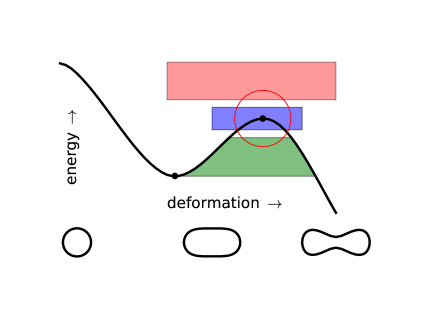
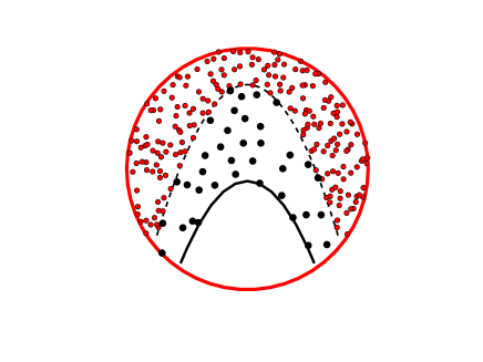
Figure 1: The fission barrier. Top: the black line depicts the potential energy surface (PES) as a function of some deformation parameter associated with the shape change during fission. The left-most black dot on the PES indicates the moderately deformed ground state. The other black dot on the PES indicates the barrier top. The shaded areas show regions of different shape dynamics. In the ground state and at low excitation energy, fission occurs by tunneling through the barrier (green area). At sufficiently high energy, diffusive dynamics is expected (red area). The region just around the barrier top (blue area) shows strong fluctuations and is the subject of the present study. Bottom: a magnified view of the circled barrier-top region in a discrete-basis representation. Configurations are indicated by dots. The solid black line is the PES near the barrier top. We distinguish regions in the energy-deformation plane with low and high level densities. The high level-density regions are modeled by random matrix theory; the the levels in the low-density region at the barrier must be treated explicitly.

There is also a residual interaction between the configurations that is responsible for the dynamics. The important point for the discrete basis representation is that that a two-body residual interaction cannot change the shape by a a large amount, so the couplings are of limited range on the horizontal scale.

At excitation energies relevant for the fission dynamics in nuclear reactors, the configurations at the initial deformation form a compound nucleus. This means that the residual interactions produce a statistical distribution of amplitudes and energies as in random matrix theory. The statistical limit is approached when the residual interactions are uncorrelated and on average larger then the energy spacing between the levels zi83 . While this limit is achieved on the right and left-hand sides at moderate excitation energy, it will not be the case for configurations in the middle, at energies around the barrier energy.

We thus a led to a Hamiltonian that consists of of two statistical reservoirs connected by a set of bridge configurations. This already simplifies the dynamics greatly. One first determines the boundaries of the reservoirs by calculation the level densities and average interaction energies as a function of energy and the shape parameter. The interactions of the bridge configurations still has to be determined. However, the coupling to the reservoirs can be treated statistically: the only relevant parameter is the decay width into the reservoir.

For the remainder of this letter, and in order to make contact with the Eq. (1) and (2), we simplify the Hamiltonian to a single bridge state together with the the reservoirs. The time-dependent Schrödinger equation for the Hamiltonian will be solved numerically to find the transition rate out of the left-hand reservoir supp .

To define the Hamiltonian, we label the configurations in the left and right reservoirs by $l$ and $r$, respectively. The bridge configuration is labeled by $b$. The non-zero matrix elements of the Hamiltonian are: $\langle l|H|l^{\prime}\rangle=\delta_{l,l^{\prime}}E_{l}$, $\langle r|H|r^{\prime}\rangle=\delta_{r,r^{\prime}}E_{r}$, $\langle l|H|b\rangle=v_{lb}$, $\langle r|H|b\rangle=v_{rb}$, and $\langle b|H|b\rangle=E_{b}.$.

We first demonstrate that Eq. (2) of the mesoscopic theory can be recovered by taking equally spaced levels in the reservoirs and constant values for the coupling matrix elements. We denote the parameters as $v_{L}=v_{lb},v_{R}=v_{rb},\Delta E_{L}=E_{l}-E_{l-1}$ and $\Delta E_{R}=E_{r}-E_{r-1}$. It is convenient to define decay widths of the bridge state to the right and left by Fermi’s Golden Rule, $\Gamma_{L,R}=2\pi v^{2}_{L,R}/\Delta E_{L,R}$. As an example, we show in Fig. 2 (solid line) the survival probability in the left-hand reservoir starting from an initial wave function that is an eigenstate in the middle of the spectrum of that reservoir. The Hamiltonian parameters are given in Figure caption.

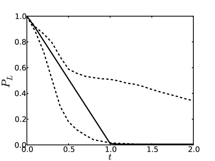
Figure 2: Survival probability in the left-hand reservoir as a function of time. Solid black line: regular Hamiltonians in both reservoirs. The numerical Hamiltonian has 100 and 200 levels in the left- and right-hand reservoirs respectively with the same bandwidths. The coupling matrix elements are chosen so that $\Gamma_{L}=\Gamma_{R}$ and $\Gamma_{L}/\Delta E_{L}=0.12N_{L}$. The energy of the bridge state is taken equal to the initial state. Dashed lines: two examples of decays when diagonal energies of the left-hand Hamiltonian are taken from random matrix theory. The time $t$ is given in units of $t_{0}$, Eq. (3).

One sees that the survival probability decreases linearly with time at a rate $W=\Delta E_{L}/2\pi$ up to the characteristic time

$$t_{0}={2\pi\over\Delta E_{L}}.$$ (3)

This is in perfect agreement with the combined Eq. (1) and (2), since $T=1$ for the given parameters. It may seem surprising that the probability current is constant up to the time $t_{0}$, but this can be easily understood. The uniform spacing of the levels in the left-hand reservoir simulates the middle of a band in a perfect one-dimensional conducting wire. The wave function of an eigenstate of the isolated wire has the particle uniformly distributed over the length of the wire, and equal currents flowing to the left and to the right. When the interaction with the bridge state is turned on, the right-moving current passes without impediment to the other reservoir. The current only goes to zero after twice the transit time of the wire. If the parameters are changed so that $T<1$, the only difference up to a time $t_{0}$ is that the slope changes from $t_{0}^{-1}$ to $T/t_{0}$.

We now go to Hamiltonians closer to the nuclear cases, modifying the reservoirs according to random matrix theory. In fact, we found that the physics associated with the right-hand reservoir is insensitive to the fine details of its Hamiltonian. The levels spacings can be taken to be uniform or as extracted from the middle levels from Wigner’s random matrix ensemble. The coupling matrix elements $v_{rb}$ can be constant or Gaussian distributed, again from Wigner’s random matrix ensemble. The only important properties are:

$\bullet$ The width $\Gamma_{R}$. It may be computed from the Fermi Golden Rule using average level density and the root-mean-square average interaction matrix element.
$\bullet$ The average level spacing must be smaller than any other energy scale (or inverse time scale).

Under these conditions the coupling to the right-hand reservoir can be treated very simply. Instead of including it explicitly in the Hamiltonian, the absorptive effect of the right-hand reservoir can be computed adding an imaginary potential $-i\Gamma_{R}/2$ to $\langle b|H|b\rangle$. We have adopted this simplification for computing the rates shown below.

In sharp contrast to the results for uniform level spacing in the left-hand reservoir, the decay properties are quite different with reservoir governed by random matrix theory. One aspect is well-understood: the decay width of a state $l$ is proportional to the square of the coupling matrix element $v_{lb}$ which has a Gaussian distribution in random matrix models. This is called the Porter-Thomas distribution. But there is more. Fig. 2 shows two decay distributions when the level spectrum $E_{l}$ was taken from a random matrix ensemble but with constant coupling matrix elements, as in the quantum wire. One sees that the decay rates do not have any simple behavior; they can neither be described as constant or as exponential decays.

For the physical problem we only care about the averages over many initial states. Fig. 3 shows such an average, for conditions that correspond to a unit transmission coefficient, $\Gamma_{L}=\Gamma_{R}$ and $E=E_{b}$.

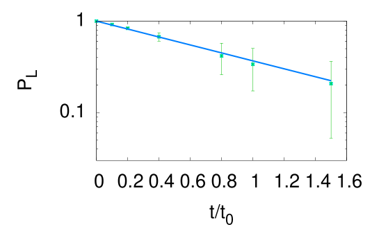
Figure 3: Survival probability in the the left-hand reservoir averaged over the random statistical ensemble of reservoir Hamiltonians but with a constant coupling to the bridge state. Squares show the average values and error bars show the the root-mean-square deviation of individual decay probabilities. Solid line is the exponential function $\exp(-Wt)$ with $W$ from Eq. (1).

The average follows very well an exponential decay law, with an average decay rate given by Eq. (1). The error bars show the root mean square deviation of the individual probabilities $P(t)$; one sees that there are large fluctuations about the average. We have also examined the dependence of the decay profiles $P(t)$ on $\Delta E_{L}$, $v_{L}$, and $E_{b}$ and found that the average profiles are exponential and fairly well described by the formula

$$\overline{\Gamma}_{c}={1\over 2\pi\rho_{I}}{\Gamma_{R}\Gamma_{L}\over E_{b}^{2}+(\Gamma_{R}+\Gamma_{L})^{2}/4}.$$ (4)

As a final step to apply random matrix distributions to the left-hand reservoir, we taking the coupling strengths $v_{bL}$ to be Gaussian distributed with variance $\langle v^{2}_{bL}\rangle=v_{0}^{2}$. The expected average survival probability is then given by

$$\overline{P}(t)={1\over(2\pi v_{0})^{1/2}}\int_{-\infty}^{\infty}dve^{-v^{2}/2v_{0}^{2}-2\pi v^{2}\rho_{I}t}={1\over(1+2\Gamma_{0}t)^{1/2}},$$ (5)

where $\Gamma_{0}=2\pi v_{0}^{2}\rho_{I}$. Fig. 4 shows the computed $\overline{P}(t)$ as black dots, taking parameters such than $T_{b}=1$. It agrees very well with Eq. (5), shown as the solid line in the Figure. For these parameters, $\Gamma_{0}=1/2\pi\rho_{I}=t_{0}^{-1}$.

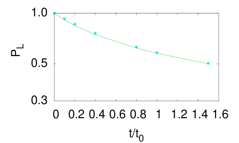
Figure 4: Squares show the survival probability in the left-hand reservoir averaged over the random ensemble of Hamiltonians, including the random distribution of couplings to the bridge state. Eq. (5) is shown as the solid line.

A hallmark of the present approach would be the observation of fluctuations in the fission transmission function above the barrier that could be ascribed to individual bridge states. This would require that the density of bridge states not be too large compared to the decay widths of the states. Detailed calculations of the coupling matrix elements may be required to see if that is likely for the lowest states.

Experimentally mo78 , large-amplitude fluctuations have been seen in the suprabarrier fission of ²³⁶U on the scale of 1 keV . The amplitude of the fluctuation in $T$ is of the order 1, which is consistent with a resonant mechanism. However, the spacing of bridge states would be much larger than 1 keV, since the excitation energies of the observed fluctuations is only 1 MeV above the barrier. In fact, these fluctuations can be accounted for as statistical in origin, arising from the Porter-Thomas fluctuations of decays of the intermediate states in the fission process mo84 .

The discussion in the above paragraph hints at the many complications that are present in making a more realistic description of fission. We mention two of the important ingredients for a predictive theory that have been neglected here. The first is that the barrier region very likely requires many bridge configurations to be considered explicitly. The fission barrier has at least two humps br72 . Besides bridge states crossing the two humps, the intermediate states, called class II states, are visible as closely-spaced resonances in the fission excitation functions. Once we go beyond the individual bridge state linking the two reservoirs, the properties of the interaction linking the bridge states becomes very important. It is well-known that in the sub-barrier region the fission lifetimes are very sensitive to the pairing interaction ro14 . This gives a coherence to the matrix elements of the lowest bridge states, and if the pairing strength were large enough would allow the linked states to act as channels. However, nuclear pairing is rather weak and is easy blocked in excited states. For that reason, the discrete basis picture may be closer to the physical reality than the channel picture.

Acknowledgments. This work arose out of discussions in the program “Quantitative large amplitude dynamics” at the Institute for Nuclear Theory, with especial thanks to W. Nazarewicz for encouraging this line of inquiry. The author also thanks Y. Alhassid and R. Vandenbosch for helpful discussions. Finally, the author thanks P. Talou and O. Bouland for pointing out the importance of the statistical mechanism to introduce fluctuations in the suprabarrier transmission function. Research was support by the DOE under Grant No. FG02-00ER41132.

References

- (1) N. Bohr and J.A. Wheeler, Phys. Rev. 56 426.
- (2) S. Bjornholm and J.E. Lynn, Rev. Mod. Phys. 52 725 (1980).
- (3) O. Bouland, J.E. Lynn, and P. Talou, Phys. Rev. C 88 054612 (2013).
- (4) O. Bouland, J.E. Lynn, and P. Talou, Nucl. Data Sheets 118 211 (2014).
- (5) B.J. van Wees, et al. Phys. Rev. Lett. 60 848 (1988)
- (6) Y. Alhassid, Rev. Mod. Phys. 72 895 (2000).
- (7) R. Landauer, IBM J. Res. Dev. 1 223 (1957).
- (8) M. Bender, P.-H. Heenen, and P-G. Reinhard, Rev. Mod. Phys. 75 121 (2003).
- (9) M. Zirnbauer, J. Verbaarschot, and H.A. Weidenmüller, Nucl. Phys. A411 161 (1983).
- (10) The computer codes used for the numerical solution of the time-dependent Schrödinger equation and to generate the input data files for the figures is provided in the article’s Supplementary Material.
- (11) R. Rodriguez-Guzmann and L.M. Robledo, Phys. Rev. C 89 054310 (2014).
- (12) J. Randrup and P. Möller, Phys. Rev. Lett. 106 132503 (2011).
- (13) G.F. Bertsch,J. Phys. Condens. Matter 3 373 (1991).
- (14) R.B. Perez, G. de Saussure, E.G. silver, R.W. Ingle, and H. Weaver, Nucl. Sci. Eng. 55 203 (1974).
- (15) M.S. Moore, J.D Moses, G.A. Keyworth, J.W. Dobbs and N.W.Hill, Phys. Rev. C 18 1328 (1978).
- (16) M.S. Moore, L. Calabretta, F. Corvi, and H. Weigmann, Phys. Rev. C 30 214 (1984).
- (17) M. Brack, et al., Rev. Mod. Phys. 44 320 (1972).