Event–Selected Vector Field Discontinuities Yield Piecewise–Differentiable Flows

Abstract

We study a class of discontinuous vector fields brought to our attention by multi–legged animal locomotion. Such vector fields arise not only in biomechanics, but also in robotics, neuroscience, and electrical engineering, to name a few domains of application. Under the conditions that (i) the vector field’s discontinuities are locally confined to a finite number of smooth submanifolds and (ii) the vector field is transverse to these surfaces in an appropriate sense, we show that the vector field yields a well–defined flow that is Lipschitz continuous and piecewise–differentiable. This implies that although the flow is not classically differentiable, nevertheless it admits a first–order approximation (known as a Bouligand derivative) that is piecewise–linear and continuous at every point. We exploit this first–order approximation to infer existence of piecewise–differentiable impact maps (including Poincaré maps for periodic orbits), show the flow is locally conjugate (via a piecewise–differentiable homeomorphism) to a flowbox, and assess the effect of perturbations (both infinitesimal and non–infinitesimal) on the flow. We use these results to give a sufficient condition for the exponential stability of a periodic orbit passing through a point of multiply intersecting events, and apply the theory in illustrative examples to demonstrate synchronization in abstract first– and second–order phase oscillator models.

1 Introduction

We study a class of discontinuous vector fields brought to our attention by multi–legged animal locomotion. Parsimonious dynamical models for diverse physical phenomena are governed by vector fields that are smooth except along a finite number of surfaces of discontinuity. Examples include: integrate–and–fire neurons that undergo a discontinuous change in membrane voltage during a threshold crossing [Kee+81, HH95, Biz+13]; legged locomotors that encounter discontinuities in net forces due to intermittent interaction of viscoelastic limbs with terrain [Ale84, Gol+99, Hol+06]; electrical power systems that undergo discontinuous changes in network topology triggered by excessive voltages or currents [His95]. In each of these examples, behaviors of interest—phase locking [Kee+81] or local synchronization [HH95]; simultaneous touchdown of two or more legs [Ale84, Gol+99, Hol+06]; voltage collapse phenomena [DL92] [His95, Section II-A.2]—occur at or near the intersection of multiple surfaces of discontinuity. Although analytical tools exist to study orbits that pass transversely through non–intersecting switching surfaces (e.g. to assess stability [AG58, Gri+02], compute first–order variations [HP00, WA12], and reduce dimensionality [Bur+15a]), piecewise–defined (or hybrid) systems that admit simultaneous discrete transitions generally exhibit “branching” wherein the flow depends discontinuously on initial conditions [Sim+05, Definition 3.11]. For instance, in the mechanical setting, the flow of a Lagrangian dynamical system subject to unilateral constraints is generically discontinuous near simultaneous–impact events [Bal00, Section 7]. In the case where a vector field is discontinuous across two transversally–intersecting surfaces, others have established continuity and derived first–order approximations of the flow [Iva98, DB+08, DL11, Biz+13]. Techniques applicable to arbitrary numbers of surfaces have been derived for the case of pure phase oscillators with perpendicular transition surfaces [MS90].

We generalize these approaches to accommodate an arbitrary number of nonlinear transition surfaces that are not required to be transverse and extend a suite of analytical and computational techniques from classical (smooth) dynamical systems theory to the present (non–smooth) setting. Under the conditions that (i) the vector field’s discontinuities are locally confined to a finite collection of smooth submanifolds and (ii) the vector field is “transverse” to these surfaces in an appropriate sense, we show that the vector field yields a well–defined flow that is Lipschitz continuous and piecewise–differentiable. The definition of piecewise–differentiability we employ (introduced in [Rob87, Roc03, Sch12]) implies that although the flow is not classically differentiable, nevertheless it admits a first–order approximation (the so–called Bouligand derivative or B–derivative [Sch12, Chapter 3]) that is piecewise–linear and continuous at every point. We exploit this first–order approximation to infer existence of piecewise–differentiable impact maps (including Poincaré maps for periodic orbits), assess the effect of perturbations on the flow, and derive a straightforward procedure to compute the B–derivative. We use these results to give a sufficient condition for the exponential stability of a periodic orbit passing through a point of multiply intersecting events, and apply the theory in illustrative examples to demonstrate synchronization in abstract first– and second–order phase oscillator models.

The paper is organized as follows. Following a brief review of relevant technical background in Section 2, we define the discontinuous but piecewise–smooth vector fields of interest and show that they yield continuous B–differentiable flows in Section 3. In Section 4 we demonstrate that such flows are continuously conjugate to classical flows, leading to results in Section 5 establishing their persistence under small perturbations. Section 6 develops stability results and their application to simple oscillator models is given in Section 7. The paper concludes with a brief summary in Section 8 suggesting the relevance of these results to biological and engineered systems of practical interest.

2 Preliminaries

The mathematical constructions we use are “standard” in the sense that they are familiar to practitioners of (applied) dynamical systems or optimization theory (or both), but since this paper represents (to the best of our knowledge) the first application of some techniques from non–smooth analysis to the present class of dynamical systems, the reader may be unfamiliar with some of the more recently–developed devices we employ. Thus in this section we briefly review mathematical concepts and introduce notation that will be used to state and prove results throughout this paper, and suggest textbook references where the interested reader could obtain a complete exposition.

2.1 Notation

To simplify the statement of our definitions and results, we fix notation of some objects in $\mathbb{R}^{n}$: $+\mathds{1}\in\mathbb{R}^{n}$ denotes the vector of all ones and $-\mathds{1}$ its negative; $e_{j}$ is the $j$–th standard Euclidean basis vector; $B_{n}:=\left\{-1,+1\right\}^{n}\subset\mathbb{R}^{n}$ is the set of corners of the $n$-dimensional cube. We let $\operatorname{sign}:\mathbb{R}^{n}\rightarrow\left\{-1,+1\right\}^{n}$ be the vectorized signum function taking its values in the Euclidean cube’s corners, i.e.

$$\forall x\in\mathbb{R}^{n},j\in\left\{1,\dots,n\right\}:e_{j}^{\top}\operatorname{sign}(x)=\left\{\begin{array}[]{ll}-1,&x_{j}<0\\ +1,&x_{j}\geq 0\end{array}\right..$$ (1)

To fix notation, in the following paragraphs we will briefly recapitulate standard constructions from topology, differential topology, and dynamical systems theory, and refer the reader to [Lee12] for details. If $U\subset X$ is a subset of a topological space, then $\operatorname{Int}U\subset X$ denotes its interior and $\partial U$ denotes its boundary. Let $f:X\rightarrow Y$ be a map between topological spaces. If $U\subset X$ then $f|_{U}:U\rightarrow Y$ denotes the restriction. If $V\subset Y$ then $f^{-1}(V)=\left\{x\in X:f(x)\in V\right\}$ denotes the pre–image of $V$ under $f$.

Given $C^{r}$ manifolds $D,N$, we let $C^{r}(D,N)$ denote the set of $C^{r}$ functions from $D$ to $N$. $H\subset D$ is a $C^{r}$ codimension-$k$ submanifold of the $d$-dimensional manifold $D$ if every $x\in H$ has a neighborhood $U\subset D$ over which there exists a $C^{r}$ diffeomorphism $h:U\rightarrow\mathbb{R}^{d}$ such that

$$H\cap U=h^{-1}\left(\left\{y\in\mathbb{R}^{d}:y_{k+1}=\cdots=y_{d}=0\right\}\right).$$

If $f\in C^{r}(D,N)$ then at every $x\in D$ there exists an induced linear map $Df(x):T_{x}D\rightarrow T_{f(x)}N$ called the pushforward (in coordinates, $Df(x)$ is the Jacobian linearization of $f$ at $x\in D$) where $T_{x}D$ denotes the tangent space to the manifold $D$ at the point $x\in D$. Globally, the pushforward is a $C^{r-1}$ map $Df:TD\rightarrow TN$ where $TD$ is the tangent bundle associated with the manifold $D$; we recall that $TD$ is naturally a $2d$–dimensional $C^{r}$ manifold. When $N=\mathbb{R}$, we will invoke the standard identification $T_{y}N\simeq\mathbb{R}$ for all $y\in N$ and regard $Df(x)$ as a linear map from $T_{x}D$ (i.e. an element of the cotangent space $T_{x}^{*}D$) into $\mathbb{R}$ for every $x\in D$; we recall that the cotangent bundle $T^{*}D$ is naturally a $2d$–dimensional $C^{r}$ manifold. If $U\subset D$ and $f:U\rightarrow N$ is a map, then a map $\widetilde{f}:D\rightarrow N$ is a $C^{r}$ extension of $f$ if $\widetilde{f}$ is $C^{r}$ and $\widetilde{f}|_{U}=f$.

Following [Lee12, Chapter 8], a (possibly discontinuous or non–differentiable) map $F:D\rightarrow TD$ is a (rough) vector field if $\pi\circ F=\operatorname{id}_{D}$ where $\pi:TD\rightarrow D$ is the natural projection and $\operatorname{id}_{D}$ is the identity map on $D$. A vector field may, under appropriate conditions, yield an associated flow $\phi:\mathscr{F}\rightarrow D$ defined over an open subset $\mathscr{F}\subset\mathbb{R}\times D$ called a flow domain; in this case for every $x\in D$ the set $\mathscr{F}^{x}=\mathscr{F}\cap\left(\mathbb{R}\times\left\{x\right\}\right)$ is an open interval containing the origin, the restriction $\phi|_{\mathscr{F}^{x}}:\mathscr{F}^{x}\rightarrow D$ is absolutely continuous, and the derivative with respect to time is $D_{t}\phi(t,x)=F(\phi(t,x))$ for almost every $t\in\mathscr{F}^{x}$. A flow is maximal if it cannot be extended to a larger flow domain. An integral curve for $F$ is an absolutely continuous function $\xi:I\rightarrow D$ over an open interval $I\subset\mathbb{R}$ such that $\dot{\xi}(t)=F(\xi(t))$ for almost all $t\in I$; it is maximal if it cannot be extended to an integral curve on a larger open interval.

2.2 Piecewise Differentiable Functions and Nonsmooth Analysis

The notion of piecewise–differentiability we employ was originally introduced by Robinson [Rob87]; since the recent monograph from Scholtes [Sch12] provides a more comprehensive exposition, we adopt the notational conventions therein. Let $r\in\mathbb{N}\cup\left\{\infty\right\}$ and $D\subset\mathbb{R}^{d}$ be open. A continuous function $f:D\rightarrow\mathbb{R}^{n}$ is called piecewise–$C^{r}$ if for every $x\in D$ there exists an open set $U\subset D$ containing $x$ and a finite collection $\left\{f_{j}:U\rightarrow\mathbb{R}^{n}\right\}_{{j}\in\mathscr{J}}$ of $C^{r}$–functions such that for all $x\in U$ we have $f(x)\in\left\{f_{j}(x)\right\}_{{j}\in\mathscr{J}}$. The functions $\left\{f_{j}\right\}_{{j}\in\mathscr{J}}$ are called selection functions for $f|_{U}$, and $f$ is said to be a continuous selection of $\left\{f_{j}\right\}_{j\in\mathscr{J}}$. A selection function $f_{j}$ is said to be active at $x\in U$ if $f(x)=f_{j}(x)$. We let $PC^{r}(D,\mathbb{R}^{n})$ denote the set of piecewise–$C^{r}$ functions from $D$ to $\mathbb{R}^{n}$. Note that $PC^{r}$ is closed under composition and pointwise maximum or minimum of a finite collection of functions. Any $f\in PC^{r}(D,\mathbb{R}^{n})$ is locally Lipschitz continuous, and a Lipschitz constant for $f$ is given by the supremum of the induced norms of the (Fréchet) derivatives of the set of selection functions for $f$. Piecewise–differentiable functions possess a first–order approximation $Df:TD\rightarrow T\mathbb{R}^{n}$ called the Bouligand derivative (or B–derivative) [Sch12, Chapter 3]; this is the content of Lemma 4.1.3 in [Sch12]. We let $Df(x;v)$ denote the B–derivative of $f$ evaluated along the tangent vector $v\in T_{x}D$. The B–derivative is positively homogeneous, i.e. $\forall v\in T_{x}D,\lambda\geq 0:Df(x;\lambda v)=\lambda Df(x;v)$.

3 Local and Global Flow

In this section we rederive in our present nonsmooth setting the erstwhile familiar fundamental construction associated with a vector field: its flow. We begin in Section 3.1 by introducing the class of vector fields under consideration, namely, event–selected $C^{r}$ vector fields. Subsequently in Section 3.2 we construct a candidate flow function via composition of piecewise–differentiable functions. Finally in Section 3.3 we show this candidate function is indeed the flow of the event–selected $C^{r}$ vector field.

3.1 Event–Selected Vector Fields Discontinuities

The flow of a discontinuous vector field $F:D\rightarrow TD$ over an open domain $D\subset\mathbb{R}^{d}$ can exhibit pathological behaviors ranging from nondeterminism to discontinuous dependence on initial conditions. We will investigate local properties of the flow when the discontinuities are confined to a finite collection of smooth submanifolds through which the flow passes transversally, as formalized in the following definitions.

Definition 1.

Given a vector field $F:D\rightarrow TD$ over an open domain $D\subset\mathbb{R}^{d}$ and a function $h\in C^{r}(U,\mathbb{R})$ defined on an open subset $U\subset D$, we say that $h$ is an event function for $F$ on $U$ if there exists a positive constant $f>0$ such that $Dh(x)F(x)\geq f$ for all $x\in U$. A codimension–1 embedded submanifold $\Sigma\subset U$ for which $h|_{\Sigma}$ is constant is referred to as a local section for $F$.

Note that if $h$ is an event function for $F$ on a set containing $\rho\in D$ then necessarily $Dh(\rho)\neq 0$.

We will show in Section 3.3 that vector fields that are differentiable everywhere except a finite collection of local sections give rise to a well–defined flow that is piecewise–differentiable. This class of event–selected vector fields is defined formally as follows.

Definition 2.

Given a vector field $F:D\rightarrow TD$ over an open domain $D\subset\mathbb{R}^{d}$, we say that $F$ is event–selected $C^{r}$ at $\rho\in D$ if there exists an open set $U\subset D$ containing $\rho$ and a collection $\left\{h_{j}\right\}_{j=1}^{n}\subset C^{r}(U,\mathbb{R})$ such that:

1. (event functions) $h_{j}$ is an event function for $F$ on $U$ for all $j\in\left\{1,\dots,n\right\}$;

2. ($C^{r}$ extension) for all $b\in\left\{-1,+1\right\}^{n}=B_{n}$, with

   $$D_{b}:=\left\{x\in U:b_{j}(h_{j}(x)-h_{j}(\rho))\geq 0\right\},$$

   $F|_{\operatorname{Int}D_{b}}$ admits a $C^{r}$ extension $F_{b}:U\rightarrow TU$.

(Note that for any $b\in B_{n}$ such that $\operatorname{Int}D_{b}=\emptyset$ the latter condition is satisfied vacuously.) We let $EC^{r}(D)$ denote the set of vector fields that are event–selected $C^{r}$ at every $x\in D$.

For illustrations of event–selected $C^{r}$ vector fields in the plane $D=\mathbb{R}^{2}$, refer to Figures 1 and 2.

3.2 Construction of the Piecewise–Differentiable Flow

The following constructions will be used to state and prove results throughout the chapter. Suppose $F:D\rightarrow TD$ is event–selected $C^{r}$ at $\rho\in D$. By definition there exists a neighborhood $\rho\in U\subset D$ and associated event functions $\left\{h_{j}\right\}_{j=1}^{n}\subset C^{r}(U,\mathbb{R})$ that divide $U$ into regions $\left\{D_{b}\right\}_{b\in B_{n}}$ by defined by $D_{b}:=\left\{x\in U:(h_{j}(x)-h_{j}(\rho))b_{j}\geq 0\right\}$. The boundary of each $D_{b}$ is contained in the collection of event surfaces $\left\{H_{j}\right\}_{j=1}^{n}$ defined for each $j\in\left\{1,\dots,n\right\}$ by $H_{j}:=\left\{x\in U:\,h_{j}(x)=h_{j}(\rho)\right\}$. For each $j\in\left\{1,\dots,n\right\}$ and $b\in B_{n}$, we refer to the surface $H_{j}$ as an exit boundary in positive time for $D_{b}$ if $h_{j}(D_{b})\subset(-\infty,0]$; we refer to $H_{j}$ as an exit boundary in negative time if $h_{j}(D_{b})\subset[0,+\infty)$. In addition, the definition of event–selected $C^{r}$ implies that there is a collection of $C^{r}$ vector fields $\left\{F_{b}:U\rightarrow TU\right\}_{b\in B_{n}}\subset C^{r}(U,TU)$ such that $F|_{\operatorname{Int}D_{b}}=F_{b}|_{\operatorname{Int}D_{b}}$ for all $b\in B_{n}$.

3.2.1 Budgeted time–to–boundary

For each $b\in B_{n}$ with $\operatorname{Int}D_{b}\neq\emptyset$, let $\phi_{b}:\mathscr{F}_{b}\rightarrow U$ be a flow for $F_{b}$ over a flow domain $\mathscr{F}_{b}\subset\mathbb{R}\times U$ containing $(0,\rho)$; recall that $\phi_{b}\in C^{r}(\mathscr{F}_{b},U)$ since $F_{b}\in C^{r}(U,TU)$. Each $H\in\left\{H_{j}\right\}_{j=1}^{n}$ is a local section for $F$, and therefore a local section for $F_{b}$ as well. This implies $F_{b}(\rho)$ is transverse to $H$ (more precisely, $F_{b}(\rho)\not\in T_{\rho}H$), thus the Implicit Function Theorem [Lee12, Theorem C.40] implies there exists a $C^{r}$ “time–to–impact” map $\tau_{b}^{H}:U_{b}^{H}\rightarrow\mathbb{R}$ defined on an open set $U_{b}^{H}\subset D$ containing $\rho$ such that

$$\forall x\in U_{b}^{H}:(\tau_{b}^{H}(x),x)\in\mathscr{F}_{b}\ \text{and}\ \phi_{b}(\tau_{b}^{H}(x),x)\in H.$$ (2)

The collection of maps $\left\{\tau_{b}^{H}\right\}_{b\in B_{n}}$ are jointly defined over the open set $U_{b}:=\bigcap_{j=1}^{n}U_{b}^{H_{j}}$; note that $U_{b}$ is nonempty since $\rho\in U_{b}$. Any $x\in U_{b}$ can be taken to any $H\in\left\{H_{j}\right\}_{j=1}^{n}$ by flowing with the vector field $F_{b}$ for time $\tau_{b}^{H}(x)\in\mathbb{R}$. A useful fact we will recall in the sequel is that if $y=\phi_{b}(\tau_{b}(x),x)$ then

$$D\tau_{b}^{H}(x)=\frac{-Dh(y)D_{x}\phi_{b}(t,x)}{Dh(y)F_{b}(y)};$$ (3)

this follows from [HS74, §11.2].

We now define functions $\tau_{b}^{+},\tau_{b}^{-}:\mathbb{R}\times U_{b}\rightarrow\mathbb{R}$ that specify the time required to flow to the exit boundary of $D_{b}$ in forward or backward time, respectively, without exceeding a given time budget:

$$\forall(t,x)\in\mathbb{R}\times U_{b}:\tau_{b}^{+}(t,x) =\max{\left\{{0,\min\left(\left\{t\right\}\cup\left\{\tau_{b}^{H_{j}}(x):b_{j}<0\right\}_{j=1}^{n}\right)}\right\}},$$ (4)

$$\forall(t,x)\in\mathbb{R}\times U_{b}:\tau_{b}^{-}(t,x) =\min{\left\{{0,\max\left(\left\{t\right\}\cup\left\{\tau_{b}^{H_{j}}(x):b_{j}>0\right\}_{j=1}^{n}\right)}\right\}};$$

Since $\tau_{b}^{+},\tau_{b}^{-}$ are obtained via pointwise minimum and maximum of a finite collection of $C^{r}$ functions, we conclude $\tau_{b}^{+},\tau_{b}^{-}\,\in PC^{r}(\mathbb{R}\times U_{b},\mathbb{R})$. See Figure 1 for an illustration of the component functions of $\tau_{b}^{+}$ in a planar vector field.

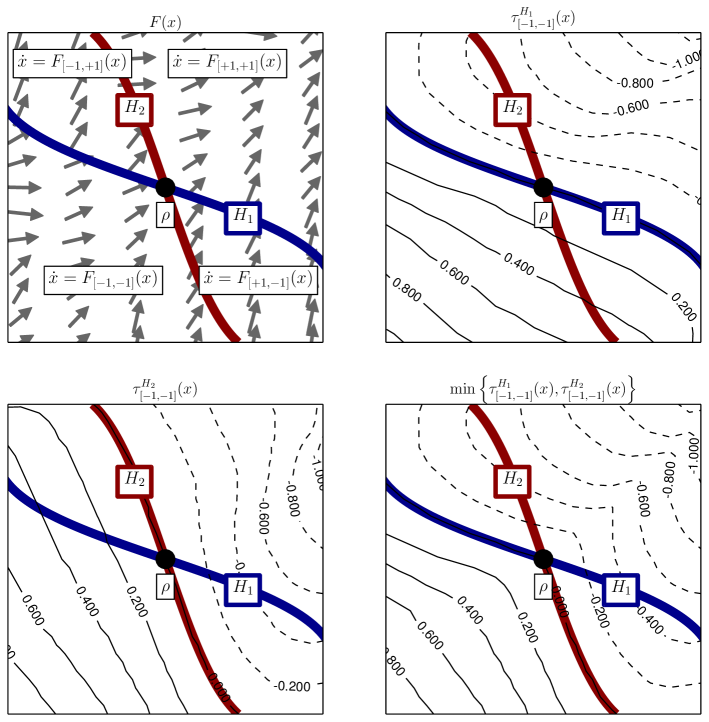
Figure 1: Illustration of a vector field $F:D\rightarrow TD$ that is event–selected $C^{r}$ at $\rho\in D=\mathbb{R}^{2}$. The functions $\left\{\tau_{[-1,-1]}^{H_{j}}\right\}_{j=1}^{2}$ specify the time required to flow via the vector field $F_{[-1,-1]}$ to the surface $H_{j}$. The pointwise minimum $\min\left\{\tau_{[-1,-1]}^{H_{j}}(x)\right\}_{j=1}^{2}$ is used in the definition of $\tau_{[-1,-1]}^{+}$ in (4).

In the sequel we will require the derivative of $\tau_{b}^{+}$ with respect to $t$ and $x$. In general this can be obtained via the chain rule [Sch12, Theorem 3.1.1]. If we define $\nu_{b}^{+}:U_{b}\rightarrow\mathbb{R}\cup\left\{+\infty\right\}$ using the convention $\min\emptyset=+\infty$ by

$$\forall x\in U_{b}:\nu_{b}^{+}(x)=\min\left\{\tau_{b}^{H_{j}}(x):b_{j}<0\right\}_{j=1}^{n},$$ (5)

then we immediately conclude that for all $(t,x)\in\mathbb{R}\times U_{b}$ such that $\nu_{b}^{+}(x)\neq t\neq 0$, the forward–time budgeted time–to–boundary $\tau_{b}^{+}$ is classically differentiable and

$$D\tau_{b}^{+}(t,x)=\left\{\begin{array}[]{ll}(0,\ 0_{d}^{\top}),&t<0;\\ (1,\ 0_{d}^{\top}),&0<t<\nu_{b}^{+}(x);\\ \left(0,D\tau_{b}^{H}(x)\right),&\nu_{b}^{+}(x)<t;\end{array}\right.$$ (6)

where in the third case $H\in\left\{H_{j}\right\}_{j=1}^{n}$ is such that $\tau_{b}^{H}(x)=\nu_{b}^{+}(x)$. To compute $D\tau_{b}^{-}(t,x)$, one may simply use the formula in (6) applied to the vector field $-F$; full details are provided in Appendix A.1.

3.2.2 Budgeted flow–to–boundary

By composing the flow $\phi_{b}$ with the budgeted time–to–boundary functions $\tau_{b}^{+},\tau_{b}^{-}$, we now construct functions that flow points up to the exit boundary of $D_{b}$ in forward or backward time over domains

$$\mathscr{V}_{b}^{+} =\left\{(t,x)\in\mathbb{R}\times U_{b}:(\tau_{b}^{+}(t,x),x)\in\mathscr{F}_{b}\right\},$$

$$\mathscr{V}_{b}^{-} =\left\{(t,x)\in\mathbb{R}\times U_{b}:(\tau_{b}^{-}(t,x),x)\in\mathscr{F}_{b}\right\}.$$

(Note that $\mathscr{V}_{b}^{+},\mathscr{V}_{b}^{-}$ are open since $\tau_{b}^{+},\tau_{b}^{-}$ are continuous and nonempty since $(0,\rho)\in\mathscr{V}_{b}^{+},\mathscr{V}_{b}^{-}$.) For each $b\in B_{n}$ define the functions $\zeta_{b}^{+}:\mathscr{V}^{+}\rightarrow D,\zeta_{b}^{-}:\mathscr{V}^{-}\rightarrow D$ by

$$\forall(t,x)\in\mathscr{V}_{b}^{+}:\zeta_{b}^{+}(t,x) =\phi_{b}\left(\tau_{b}^{+}(t,x),x\right),$$ (7)

$$\forall(t,x)\in\mathscr{V}_{b}^{-}:\zeta_{b}^{-}(t,x) =\phi_{b}\left(\tau_{b}^{-}(t,x),x\right).$$

Clearly $\zeta_{b}^{+}\in PC^{r}(\mathscr{V}_{b}^{+},D)$ and $\zeta_{b}^{-}\in PC^{r}(\mathscr{V}_{b}^{-},D)$ since they are obtained by composing $PC^{r}$ functions [Sch12, §4.1]. Loosely speaking, the function $\zeta_{b}^{+}$ coincides with $\phi_{b}$ for pairs $(t,x)$ that do not cross the forward–time exit boundary of $D_{b}$. Yet unlike $\phi_{b}$, it is the identity (stationary) flow over the remainder of its domain. More precisely, for $t<0$ and for values of $t>\nu_{b}^{+}(x)$ the function $\tau_{b}^{+}(t,x)$ is constant (and hence the derivative with respect to time $D_{t}\zeta_{b}^{+}(t,x)=0$), while for $t\in(0,\nu_{b}^{+}(x))$ we have $\zeta_{b}^{+}(t,x)=\phi_{b}(t,x)$ (and hence $D_{t}\zeta_{b}^{+}(t,x)=F_{b}(\phi_{b}(t,x))$).

Now fix $x\in D_{b}$, choose $a\in B_{n}\setminus{b}$, and for $t\in\mathbb{R}$ define

$$t_{a}^{+}(t):=\min\left\{\tau_{a}^{H_{j}}\left(\zeta_{b}^{+}(t,x)\right):{a}_{j}<0\right\}_{j=1}^{n}.$$

Applying the conclusions from the preceding paragraph, with $t^{\prime}\in\mathbb{R}$ the composition

$$\zeta_{a}^{+}(t^{\prime},\zeta_{b}^{+}(t,x))$$

is classically differentiable with respect to both $t^{\prime}$ and $t$ almost everywhere. Furthermore, we can deduce that the derivative of the composition with respect to $t$ is $F_{b}(\phi_{b}(t,x))$ when $t\in\left(0,\nu_{b}^{+}(x)\right)$ and zero where it is otherwise defined; similarly, the derivative with respect to $t^{\prime}$ is $F_{a}\left(\phi_{a}(t^{\prime},\zeta_{b}^{+}(t,x)\right)$ when $t^{\prime}\in\left(0,t_{a}^{+}(t)\right)$ and zero where it is otherwise defined. If we impose the relationship $t^{\prime}:=t-\tau_{b}^{+}(t,x)$, we have $t^{\prime}=0$ for any $t\in(0,\nu_{b}^{+}(x))$. The composition

$$\zeta_{a}^{+}(t-\tau_{b}^{+}(t,x),\zeta_{b}^{+}(t,x))$$

follows the flow for $F_{b}$ from $x$ toward (but never passing) the exit boundary of $D_{b}$, then follows the flow of $F_{a}$ from $\zeta_{b}^{+}(t,x)$ toward the exit boundary of $D_{a}$.

In the sequel we will require the derivative of $\zeta_{b}^{+}$ with respect to $t$ and $x$. In general this can be obtained via the chain rule [Sch12, Theorem 3.1.1]. If we define $\nu_{b}^{+}:U_{b}\rightarrow\mathbb{R}$ as in (5) then we immediately conclude that for all $(t,x)\in\mathbb{R}\times U_{b}$ such that $\nu_{b}^{+}(x)\neq t\neq 0$, the forward–time flow–to–boundary $\zeta_{b}^{+}$ is classically differentiable and

$$D\zeta_{b}^{+}(t,x)=\left\{\begin{array}[]{ll}(0_{d},\ 0_{d\times d}),&t<0;\\ (F_{b}(\phi_{b}(t,x)),\ D_{x}\phi_{b}(t,x)),&0<t<\nu_{b}^{+}(x);\\ (0_{d},\Upsilon(t,x)),&\nu_{b}^{+}(x)<t;\end{array}\right.$$ (8)

where in the third case $\Upsilon(t,x)={\left(0,F_{b}(\phi_{b}(\tau_{b}^{+}(t,x),x))D\tau_{b}^{H}(x)+D_{x}\phi_{b}(\tau_{b}^{+}(t,x),x)\right)}$ and $H\in\left\{H_{j}\right\}_{j=1}^{n}$ is such that $\tau_{b}^{H}(x)=\nu_{b}^{+}(x)$. To compute $D\zeta_{b}^{-}(t,x)$, one may simply use the formula in (8) applied to the vector field $-F$; full details are provided in Appendix A.2.

3.2.3 Composite of budgeted time–to– and flow–to–boundary

Define $\varphi_{b}^{+}:\mathscr{V}_{b}^{+}\rightarrow\mathbb{R}\times D$, $\varphi_{b}^{-}:\mathscr{V}_{b}^{-}\rightarrow\mathbb{R}\times D$ by

$$\forall(t,x)\in\mathscr{V}_{b}^{+}:\varphi_{b}^{+}(t,x) =\left(t-\tau_{b}^{+}(t,x),\zeta_{b}^{+}(t,x)\right)=\left(t-\tau_{b}^{+}(t,x),\phi_{b}\left(\tau_{b}^{+}(t,x),x\right)\right),$$ (9)

$$\forall(t,x)\in\mathscr{V}_{b}^{-}:\varphi_{b}^{-}(t,x) =\left(t-\tau_{b}^{-}(t,x),\zeta_{b}^{-}(t,x)\right)=\left(t-\tau_{b}^{-}(t,x),\phi_{b}\left(\tau_{b}^{-}(t,x),x\right)\right).$$

Clearly $\varphi_{b}^{+}\in PC^{r}(\mathscr{V}_{b}^{+},\mathbb{R}\times D)$ and $\varphi_{b}^{-}\in PC^{r}(\mathscr{V}_{b}^{-},\mathbb{R}\times D)$. Intuitively, the second component of the $\varphi_{b}^{+}$, $\varphi_{b}^{-}$ functions flow according to $F_{b}$ up to exit boundaries of $D_{b}$ in forward or backward time, respectively, while the first component deducts the flow time $t-\tau_{b}^{\pm}(t,x)$ from the total time budget $t$. These functions satisfy an invariance property:

$$\forall(t,x)\in\left(\mathscr{V}_{b}^{+}\cap(-\infty,0]\times U_{b}\right) :\varphi_{b}^{+}(t,x)=(t,x),$$ (10)

$$\forall(t,x)\in\left(\mathscr{V}_{b}^{-}\cap[0,+\infty)\times U_{b}\right) :\varphi_{b}^{-}(t,x)=(t,x).$$

We now combine (6) and (8) to obtain the derivative of $\varphi_{b}^{+}$ for all $(t,x)\in\mathbb{R}\times U_{b}$ such that $\nu_{b}^{+}(x)\neq t\neq 0$:

$$D\varphi_{b}^{+}(t,x)=\left\{\begin{array}[]{ll}\left[\begin{array}[]{cc}1&0_{d}^{\top}\\ 0_{d}&I_{d}\end{array}\right],&t<0;\\ \left[\begin{array}[]{cc}0&0_{d}^{\top}\\ F_{b}(\phi_{b}(t,x))&D_{x}\phi_{b}(t,x)\end{array}\right],&0<t<\nu_{b}^{+}(x);\\ \left[\begin{array}[]{cc}1&-D\tau_{b}^{H}(x)\\ 0_{d}&\Upsilon(t,x)\end{array}\right],&\nu_{b}^{+}(x)<t;\end{array}\right.$$ (11)

where in the third case $\Upsilon(t,x)={F_{b}(\phi_{b}(\tau_{b}^{+}(t,x),x))D\tau_{b}^{H}(x)+D_{x}\phi_{b}(\tau_{b}^{+}(t,x),x)}$ and $H\in\left\{H_{j}\right\}_{j=1}^{n}$ is such that $\tau_{b}^{H}(x)=\nu_{b}^{+}(x)$. To compute $D\varphi_{b}^{-}(t,x)$, one may simply use the formula in (8) applied to the vector field $-F$; full details are provided in Appendix A.3.

3.2.4 Construction of flow via composition

Consider now the formal composition

$$\phi=\pi_{2}\circ\left(\prod_{b=-\mathds{1}}^{+\mathds{1}}\varphi_{b}^{+}\right)\circ\left(\prod_{b=+\mathds{1}}^{-\mathds{1}}\varphi_{b}^{-}\right)$$ (12)

where $\pi_{2}:\mathbb{R}\times D\rightarrow D$ is the canonical projection and $\prod_{b=-\mathds{1}}^{+\mathds{1}}$ denotes composition in lexicographic order (similarly $\prod_{b=+\mathds{1}}^{-\mathds{1}}$ denotes composition in reverse lexicographic order). The set $\phi^{-1}(D)\subset\mathbb{R}\times D$ is open (since $\phi$ is continuous) and nonempty (since combining (10) and (12) implies $\phi(0,\rho)=\rho$). Therefore there exist open neighborhoods $J\subset\mathbb{R}$ of $0$ and $V\subset D$ of $\rho$ such that $\mathscr{F}=J\times V\subset\phi^{-1}(D)$. Clearly $\phi\in PC^{r}(\mathscr{F},D)$ since it is obtained by composing $PC^{r}$ functions. Its derivative can be computed by applying the chain rule [Sch12, Theorem 3.1.1]; alternatively, it can be obtained for almost all $(t,x)\in\mathscr{F}$ as a product of the appropriate matrices given in (11), (91). The derivative with respect to time has a particularly simple form almost everywhere, as we demonstrate in the following Lemma.

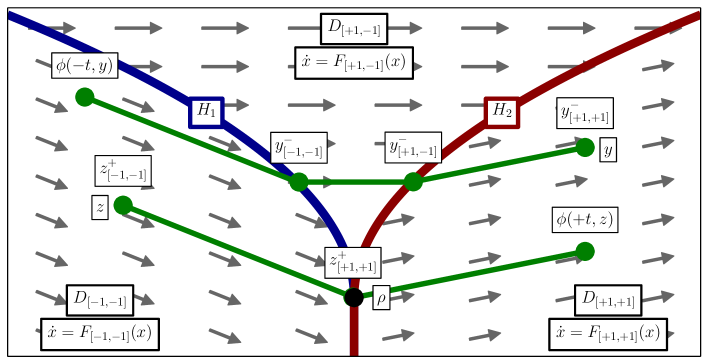
Figure 2: Illustration of a vector field $F:D\rightarrow TD$ that is event–selected $C^{r}$ near $\rho\in D=\mathbb{R}^{2}$. The vector field is discontinuous across the $C^{r}$ codimension–1 submanifolds $H_{1},H_{2}\subset D$. For each $b\in B_{n}=\left\{[-1,-1],[+1,-1],[-1,+1],[+1,+1]\right\}$, if $\operatorname{Int}D_{b}\neq\emptyset$ then the vector field restricts as $F|_{\operatorname{Int}D_{b}}=F_{b}|_{\operatorname{Int}D_{b}}$ where $F_{b}:U_{b}\rightarrow TU_{b}$ is a smooth vector field over a neighborhood $\rho\in U_{b}\subset D$. An initial condition $z\in D_{[-1,-1]}$ flows in forward time to $\phi(+t,y)\in D_{[+1,+1]}$ through $z_{[+1,+1]}^{+}\in H_{1}\cap H_{2}$. An initial condition $y\in D_{[+1,+1]}$ flows in backward time to $\phi(-t,y)\in D_{[-1,-1]}$ through $y_{[-1,+1]}^{-}\in H_{1}$ and $y_{[-1,-1]}^{-}\in H_{2}$.

Lemma 1 (time derivative of flow).

If the vector field $F:D\rightarrow TD$ is event–selected $C^{r}$ at $\rho\in D$, then for almost all $(t,x)\in\mathscr{F}$ the flow $\phi\in PC^{r}(\mathscr{F},D)$ defined by (12) is differentiable with respect to time and

$$D_{t}\phi(t,x)=F(\phi(t,x)).$$ (13)

Proof.

Choose $x\in D$ such that $(0,x)\in\mathscr{F}$. We will show that $\phi|_{\mathscr{F}^{x}}$ is classically differentiable for almost all times $t\in\mathscr{F}^{x}$. Let $t^{-}=\inf\mathscr{F}^{x}$, $t^{+}=\sup\mathscr{F}^{x}$ so that $0\in\mathscr{F}^{x}=(t^{-},t^{+})$. We construct a partition of $[0,t^{+})$ as follows. For each $b\in B_{n}$, let $(t_{b}^{+},x_{b}^{+})=\left(\prod_{a<b}\varphi_{a}^{+}\right)(t^{+},x)$ where the composition is over all $a\in B_{n}$ that occur before $b$ lexicographically; refer to Figure 2 for an illustration of the sequence $\left\{y_{b}\right\}_{b\in B_{n}}$ generated by an initial condition $y\in D_{-\mathds{1}}$. Note that $\left\{t^{+}-t_{b}^{+}\right\}_{b\in B_{n}}$ is (lexicographically) non–decreasing and $t_{+\mathds{1}}^{+}=\tau_{+\mathds{1}}^{+}(t_{+\mathds{1}}^{+},x_{+\mathds{1}}^{+})$. Defining the interval

$$J_{b}=[t^{+}-t_{b}^{+},t^{+}-t_{b}^{+}+\tau_{b}^{+}(t_{b}^{+},x_{b}^{+})],$$

we have $[0,t^{+})\subset\bigcup_{b\in B_{n}}J_{b}^{+}$ and $\operatorname{Int}J_{a}^{+}\cap\operatorname{Int}J_{b}^{+}=\emptyset$ for all $a\in B_{n}\setminus\left\{b\right\}$. Observe that

$$\forall t\in\operatorname{Int}J_{b}^{+}:\phi(t,x)=\pi_{2}\circ\varphi_{b}^{+}(t-(t^{+}-t_{b}^{+}),x_{b}^{+})\in\operatorname{Int}D_{b},$$

where the condition is vacuously satisfied if $\operatorname{Int}J_{b}^{+}=\emptyset$. Therefore for all $t\in\operatorname{Int}J_{b}^{+}$, the piecewise–differentiable function $\phi$ is classically differentiable with respect to time at $(t,x)$ and we have

$$D_{t}\phi(t,x) =D\pi_{2}\,D_{t}\varphi_{b}^{+}(t-(t^{+}-t_{b}^{+}),x_{b}^{+})$$

$$=F_{b}(\pi_{2}\circ\varphi_{b}^{+}(t-(t^{+}-t_{b}^{+}),x_{b}^{+}))$$

$$=F(\pi_{2}\circ\varphi_{b}^{+}(t-(t^{+}-t_{b}^{+}),x_{b}^{+}))$$

$$=F(\phi(t,x)).$$

Applying an analogous argument in backward time, we conclude that $D_{t}\phi(t,x)=F(\phi(t,x))$ for almost all $t\in(t^{-},t^{+})=\mathscr{F}^{x}$. Since $(0,x)\in\mathscr{F}$ was arbitrary, the Lemma follows. ∎

3.3 Piecewise–Differentiable Flow

We now show that the piecewise–differ-entiable function $\phi\in PC^{r}(\mathscr{F},D)$ defined in (12) is in fact a flow for the discontinuous vector field $F$. See Figure 2 for an illustration of this flow.

Theorem 1 (local flow).

Suppose the vector field $F:D\rightarrow TD$ is event–selected $C^{r}$ at $\rho\in D$. Then there exists a flow $\phi:\mathscr{F}\rightarrow D$ for $F$ over a flow domain $\mathscr{F}\subset\mathbb{R}\times D$ containing $(0,\rho)$ such that $\phi\in PC^{r}(\mathscr{F},D)$ and

$$\forall(t,x)\in\mathscr{F}:\phi(t,x)=x+\int_{0}^{t}F(\phi(s,x))\,ds.$$ (14)

Proof.

We claim that $\phi\in PC^{r}(\mathscr{F},D)$ from (12) satisfies (14). Applying the fundamental theorem of calculus [Sch12, Proposition 3.1.1] in conjunction with Lemma 1 and positive–homogeneity of the derivative (13), we find

$$\phi(t,x) =\phi(0,x)+\int_{0}^{1}D\phi(tu,x;t,0)du$$

$$=x+\int_{0}^{t}D\phi(s,x;t,0)\frac{1}{t}ds$$

$$=x+\int_{0}^{t}D_{t}\phi(s,x)ds$$

$$=x+\int_{0}^{t}F(\phi(s,x))ds.$$

∎

If the vector field $F:D\rightarrow TD$ is event–selected $C^{r}$ at every point in the domain $D$, we may stitch together the local flows obtained from Theorem 1 (local flow) to obtain a global flow.

Corollary 1 (global flow).

If $F\in EC^{r}(D)$, then there exists a unique maximal flow $\phi\in PC^{r}(\mathscr{F},D)$ for $F$. This flow has the following properties:

1. For each $x\in D$, the curve $\phi^{x}:\mathscr{F}^{x}\rightarrow D$ is the unique maximal integral curve of $F$ starting at $x$.

2. If $s\in\mathscr{F}^{x}$, then $\mathscr{F}^{\phi(s,x)}=\mathscr{F}^{x}-s=\left\{t-s:t\in\mathscr{F}^{x}\right\}$.

3. For each $t\in\mathbb{R}$, the set $D_{t}=\left\{x\in D:(t,x)\in\mathscr{F}\right\}$ is open in $D$ and $\phi_{t}:D_{t}\rightarrow D_{-t}$ is a piecewise–$C^{r}$ homeomorphism with inverse $\phi_{-t}$.

Proof.

This follows from a straightforward modification of the analogous Theorem 9.12 in [Lee12] (simply replace all occurrences of the word “smooth” with “$PC^{r}$”). We recapitulate the argument in Appendix C. ∎

If a vector field is event–selected $C^{r}$ at every point along an integral curve, the following Lemma shows that it is actually $C^{r}$ at all but a finite number of points along the curve.

Lemma 2 ($EC^{r}$ implies $C^{r}$ almost everywhere).

Suppose the vector field $F:D\rightarrow TD$ is event–selected $C^{r}$ at every point along an integral curve $\xi:I\rightarrow D$ for $F$ over a compact interval $I\subset\mathbb{R}$. Then there exists a finite subset $\delta\subset\xi(I)$ such that $F$ is $C^{r}$ on $\xi(I)\setminus\delta$.

Proof.

Let $\delta\subset\xi(I)$ be the set of points where $F$ fails to be $C^{r}$. If $\left|\delta\right|=\infty$, then since $\xi(I)$ is compact there exists an accumulation point $\alpha\in\xi(I)$. Since $F$ is event–selected $C^{r}$ at $\alpha$, there exists $\varepsilon>0$ such that $F$ is $C^{r}$ at every point in the set $(B_{\varepsilon}(\alpha)\cap\xi(I))\setminus\left\{\alpha\right\}$, but this violates the existence of an accumulation point $\alpha\in\delta$. Therefore $\left|\delta\right|<\infty$. ∎

Remark 1.

One of the major values of Theorem 1 (local flow) lies in the fact that piecewise–differentiable functions possess a first–order approximation called the Bouligand derivative as described in Section 2.2. This Bouligand derivative (or B–derivative) is weaker than the classical (Fréchet) derivative, but significantly stronger than the directional derivative. The B–derivative of the composition (12) can be computed by applying the chain rule [Sch12, Theorem 3.1.1].

4 Time–to–Impact, (Poincaré) Impact Map, and Flowbox

We now leverage the fact that event–selected $C^{r}$ vector fields yield piecewise–differentiable flows to obtain useful constructions familiar from classical (smooth) dynamical systems theory. Using an inverse function theorem [RS97, Corollary 20], we construct time–to–impact maps for local sections in Section 4.1. We then apply this construction to infer the existence of piecewise–differentiable (Poincaré) impact maps associated with periodic orbits in Section 4.2 and piecewise–differentiable flowboxes in Section 4.3.

4.1 Piecewise–Differentiable Time–to–Impact

We begin in this section by constructing piecewise–differentiable time–to–impact maps.

Theorem 2 (time–to–impact).

Suppose the vector field $F:D\rightarrow TD$ is event–selected $C^{r}$ at $\rho\in D$. If $\sigma\in C^{r}(U,\mathbb{R})$ is an event function for $F$ on an open neighborhood $U\subset D$ of $\rho$, then there exists an open neighborhood $V\subset D$ of $\rho$ and piecewise–differentiable function $\mu\in PC^{r}(V,\mathbb{R})$ such that

$$\forall x\in V:\sigma\circ\phi(\mu(x),x)=\sigma(\rho)$$ (15)

where $\phi\in PC^{r}(\mathscr{F},D)$ is a flow for $F$ and $(0,\rho)\in\mathscr{F}$.

Proof.

Theorem 1 (local flow) ensures the existence of a flow $\phi\in PC^{r}(\mathscr{F},D)$ such that $\mathscr{F}\subset\mathbb{R}\times D$ contains $(0,\rho)$. Let $\alpha=\sigma\circ\phi$, and note that there exist open neighborhoods $T\subset\mathbb{R}$ of $0$ and $W\subset D$ of $\rho$ such that $\alpha\in PC^{r}(T\times W,\mathbb{R})$.

We aim to apply an implicit function theorem to show that $\alpha(s,x)=\sigma(\rho)$ has a unique piecewise–differentiable solution $s=\mu(x)$ near $(0,\rho)$. To do so, we need to establish the function $\alpha$ is completely coherently oriented with respect to its first argument.

Specializing Definition 16 in [RS97], a sufficient condition for $\alpha$ to be completely coherently oriented with respect to its first argument at $(0,\rho)$ is that the (scalar) derivatives $D\alpha_{j}(0,\rho;1,0)$ of all essentially active selection functions $\left\{\alpha_{j}:j\in I^{e}(\alpha,(0,\rho))\right\}$ have the same sign. Lemma 1 implies the time derivatives of all essentially active selection functions for $\phi$ at $(0,\rho)$ are contained in the collection $\left\{F_{b}(\rho):b\in B_{n},D_{b}\neq\emptyset\right\}$ where $\left\{F_{b}:b\in B_{n}\right\}$ are the $C^{r}$ vector fields that define $F$ near $\rho$. Since $\sigma$ is an event function for $F$, there exists $f>0$ such that

$$\forall b\in B_{n}:D\sigma(\rho)F_{b}(\rho)\geq f>0.$$

This implies $\alpha$ is completely coherently oriented with respect to time at $(0,\rho)$. Therefore we may apply Corollary 20 in [RS97] to obtain an open neighborhood $0\in V\subset\mathbb{R}$ and a piecewise–differentiable function $\mu\in PC^{r}(V,\mathbb{R})$ such that (15) holds. ∎

Corollary 2 (time–to–impact).

Suppose the vector field $F:D\rightarrow TD$ is event–selected $C^{r}$ at every point along an integral curve $\xi:[0,t]\rightarrow D$ for $F$. If $\sigma\in C^{r}(U,\mathbb{R})$ is an event function for $F$ on an open set $U\subset D$ containing $\xi(t)$, then there exists an open neighborhood $V\subset D$ of $\xi(0)$ and piecewise–differentiable function $\mu\in PC^{r}(V,\mathbb{R})$ that satisfies (15).

Proof.

Corollary 1 ensures the existence of a flow $\phi\in PC^{r}(\mathscr{F},D)$ such that $\mathscr{F}\subset\mathbb{R}\times D$ contains $[0,t]\times\left\{\xi(0)\right\}$. Let $\widetilde{\mu}\in PC^{r}(\widetilde{V},\mathbb{R})$ be the time–to–impact for $\sigma$ obtained by applying Corollary 2 at $\xi(t)=\phi(t,\xi(0))$. Then with $V=\left\{x\in D:\phi(t,x)\in\widetilde{V}\right\}$, noting that $V$ is nonempty since $\xi(0)\in V$ and open since $\phi$ is continuous, the function $\mu:V\rightarrow\mathbb{R}$ defined by $\mu(x)=t+\widetilde{\mu}\circ\phi(t,x)$ is piecewise–$C^{r}$ and satisfies (15). ∎

4.2 Piecewise–Differentiable (Poincaré) Impact Map

We now apply Theorem 2 (time–to–impact) in the important case where the integral curve is a periodic orbit to construct a piecewise–differentiable (Poincaré) impact map.

Definition 3.

An integral curve $\gamma:\mathbb{R}\rightarrow D$ is a periodic orbit for the vector field $F:D\rightarrow TD$ if there exists $t>0$ such that $\gamma(t)=\gamma(0)$ and $D_{t}\gamma(s)\neq 0$ for all $s\in[0,t]$. The minimal $t>0$ for which $\gamma(t)=\gamma(0)$ is referred to as the period of $\gamma$, and we say that $\gamma$ is a $t$–periodic orbit for $F$. We let $\Gamma=\gamma(\mathbb{R})$ denote the image of $\gamma$.

Suppose the vector field $F:D\rightarrow TD$ is event–selected $C^{r}$ at every point along a $t$–periodic orbit $\gamma$ for $F$. Then given a local section $\Sigma\subset D$ for $F$ that intersects $\Gamma=\gamma(\mathbb{R})$ at $\left\{\rho\right\}=\Gamma\cap\Sigma$, Corollary 2 implies there exists a piecewise–differentiable time–to–impact $\mu\in PC^{r}(V,\mathbb{R})$ defined over an open neighborhood $V\subset D$ of $\rho$ such that $\mu(\rho)=t$. With $V\cap\Sigma$, we let $\psi:V\rightarrow\Sigma$ be the piecewise–differentiable impact map defined by

$$\forall x\in V:\psi(x)=\phi(\mu(x),x).$$ (16)

Theorem 3 (Poincaré map).

Suppose the vector field $F:D\rightarrow TD$ is event–selected $C^{r}$ at every point along a periodic orbit $\gamma$ for $F$. Then given a local section $\Sigma\subset D$ for $F$ that intersects $\Gamma=\gamma(\mathbb{R})$ at $\left\{\rho\right\}=\Gamma\cap\Sigma$, there exists an open neighborhood $V\subset D$ of $\rho$ such that the impact map (16) restricts to a piecewise–differentiable (Poincaré) map $P\in PC^{r}(S,\Sigma)$ on $S=V\cap\Sigma$.

Proof.

Without loss of generality assume $\gamma(0)\in\Sigma$. Let $T$ be the period of $\gamma$, apply Theorem 2 (time–to–impact) to $\gamma|_{[0,T]}$ to obtain an open set $V\subset D$ containing $\gamma(0)$ and a piecewise–$C^{r}$ impact time map $\mu\in PC^{r}(V,\mathbb{R})$, and define $\psi:V\rightarrow\Sigma$ as in (16). Then with $S=V\cap\Sigma$, the restriction $P=\psi|_{S}$ is a piecewise–$C^{r}$ Poincaré map for $\gamma$. ∎

Since the Poincaré map $P:S\rightarrow\Sigma$ yielded by Theorem 3 (Poincaré map) is piecewise–differentiable, it admits a first–order approximation (its Bouligand derivative) $DP:TS\rightarrow T\Sigma$ that can be used to assess local exponential stability of the fixed point $P(\rho)=\rho$. This topic will be investigated in more detail in Section 6.2.

4.3 Piecewise–Differentiable Flowbox

Theorem 2 (time–to–impact) enables us to easily derive a canonical form for the flow near an event–selected vector field discontinuity.

Theorem 4 (flowbox).

Suppose the vector field $F:D\rightarrow TD$ is event–selected $C^{r}$ at $\rho\in D$, and let $\phi:\mathscr{F}\rightarrow D$ be the flow obtained from Theorem 1 (local flow). Then there exists a piecewise–differentiable homeomorphism $\chi\in PC^{r}(V,W)$ between neighborhoods $V\subset D$ of $\rho$ and $W\subset\mathbb{R}^{d}$ of $0$ such that

$$\forall x\in V,t\in\mathscr{F}^{x}:\chi\circ\phi(t,x)=\chi(x)+te_{1}$$

where $e_{1}\in\mathbb{R}^{d}$ is the first standard Euclidean basis vector.

Proof.

Let $\sigma\in C^{r}(U,\mathbb{R})$ be an event function for $F$ on a neighborhood $\rho\in U\subset D$ that is linear. Theorem 2 (time–to–impact) implies there exists a piecewise–differentiable time–to–impact map $\mu\in PC^{r}(V,\mathbb{R})$ on a neighborhood $V\subset D$ of $\rho$ such that

$$\forall x\in V:\sigma\circ\phi(\mu(x),x)=\sigma(\rho),$$

i.e. $\phi(\mu(x),x)$ lies in the codimension–1 subspace $\Sigma=\sigma^{-1}(\sigma(\rho))$. Define $\chi:V\rightarrow\mathbb{R}\times\Sigma$ by

$$\forall x\in V:\chi(x)=(-\mu(x),\phi(\mu(x),x)).$$ (17)

Clearly $\chi\in PC^{r}(V,\mathbb{R}\times\Sigma)$ and hence $\chi$ is continuous. Furthermore, it is clear that $\chi$ is injective since (i) $\pi_{\Sigma}\chi(x)=\pi_{\Sigma}\chi(y)$ implies $x$ and $y$ lie along the same integral curve, and (ii) distinct points along an integral curve pass through $\Sigma$ at distinct times. It follows from Brouwer’s Open Mapping Theorem [Bro11, Hat02] that the image $W=\chi(V)$ is an open subset of $\mathbb{R}^{d}$. This implies $\chi$ is a homeomorphism between $V$ and $W$. With $\iota:\mathbb{R}\times\Sigma\rightarrow\mathbb{R}\times D$ denoting the canonical inclusion, the inverse of $\chi\in PC^{r}(V,W)$ is $\phi\circ\iota|_{W}\in PC^{r}(W,V)$, thus $\chi$ is a $PC^{r}$ homeomorphism. Finally, using the semi–group property of the flow $\phi$ and the fact that $\mu\circ\phi(t,x)=\mu(x)-t$ for all $x\in V,t\in\mathscr{F}^{x}$,

$$\forall x\in V,\ t\in\mathscr{F}^{x}:\chi\circ\phi(t,x) =\left(-\mu\circ\phi(t,x),\phi(\mu\circ\phi(t,x),\phi(t,x))\right)$$

$$=\left(t-\mu(x),\phi(\mu(x)-t,\phi(t,x))\right)$$

$$=\left(t-\mu(x),\phi(\mu(x),x)\right)$$

$$=\chi(x)+te_{1}.$$

∎

Thus the flow is conjugate via a piecewise–differentiable homeomorphism to a flowbox [HS74, §11.2], [Lee12, Theorem 9.22].

5 Perturbed Flow

In this section we study how the flow associated with an event–selected $C^{r}$ vector field varies under perturbations to both the smooth vector field components (in Section 5.1) and the event functions (in Section 5.2).

5.1 Perturbation of Vector Fields

Suppose $F:D\rightarrow TD$ is event–selected $C^{r}$ at $\rho\in D$ with respect to the components of $h\in C^{r}(D,\mathbb{R}^{n})$. Then by Definition 2 there exists $U\subset D$ containing $\rho$ such that for each $b\in B_{n}$ either $\operatorname{Int}D_{b}=\emptyset$ or $D_{b}\subset U$ and $F|_{\operatorname{Int}D_{b}}$ admits a $C^{r}$ extension $F_{b}:U\rightarrow TU$. We note that $F$ is determined on $U$ up to a set of measure zero from $h$ and the function $\widehat{F}\in C^{r}\left(\coprod_{b\in B_{n}}U,\coprod_{b\in B_{n}}TU\right)$ defined by $\widehat{F}|_{\left\{b\right\}\times U}=F_{b}|_{U}$. Note that we regard $C^{r}\left(\coprod_{b\in B_{n}}U,\coprod_{b\in B_{n}}TU\right)$ as a vector space under pointwise addition of tangent vectors and the norm

$$\left\|\widehat{F}\right\|_{C^{r}}=\sum_{b\in B_{n}}\left\|\widehat{F}|_{\left\{b\right\}\times U}\right\|_{C^{r}}.$$ (18)

Thus in the sequel we consider perturbations to event–selected $C^{r}$ vector fields in the space $C^{r}\left(\coprod_{b\in B_{n}}U,\coprod_{b\in B_{n}}TU\right)$.

Theorem 5 (vector field perturbation).

Let $F\in C^{r}\left(\coprod_{b\in B_{n}}D,\coprod_{b\in B_{n}}TD\right)$, $h\in C^{r}(D,\mathbb{R}^{n})$ determine an event–selected $C^{r}$ vector field at $\rho\in D$, $r\geq 1$. Then for all $\varepsilon>0$ there exists $\delta>0$ such that for all $\widetilde{F}\in B^{C^{r}}_{\delta}(F)$:

1. pairing $h$ with the perturbed vector field $\widetilde{F}$ determines an event–selected $C^{r}$ vector field at $\rho$;

2. the perturbed flow $\widetilde{\phi}:\widetilde{\mathscr{F}}\rightarrow D$ obtained by applying Theorem 1 (local flow) to this perturbed vector field satisfies $\widetilde{\phi}\in B^{C^{0}}_{\varepsilon}(\phi)$ on $\widetilde{\mathscr{F}}\cap\mathscr{F}$ and $(0,\rho)\in\widetilde{\mathscr{F}}\cap\mathscr{F}$;

3. there exists a piecewise–differentiable homeomorphism $\eta\in PC^{r}(U,\widetilde{U})$ defined between neighborhoods $U,\widetilde{U}\subset D$ of $\rho$ such that $\eta|_{B_{\delta}(\rho)}\in B^{C^{0}}_{\varepsilon}(\operatorname{id}_{B_{\delta}(\rho)})$ and we have

   $$\eta\circ\phi(t,x)=\widetilde{\phi}(t,\eta(x))$$ (19)

   for all $(t,x)\in\mathbb{R}\times\mathbb{R}^{d}$ such that $x\in U$, $t\in\mathscr{F}^{x}\cap\widetilde{\mathscr{F}}^{\eta(x)}$, and $\phi(t,x)\in U$.

Proof.

Since $F$ is event–selected $C^{r}$ with respect to $h$ at $\rho$, there exists $f>0$ such that for all $x$ sufficiently close to $\rho$ every component of $Dh(x)F(x)$ is bounded below by $f$. Then so long as $0<\delta<f$, every component of $Dh(x)\widetilde{F}(x)$ is bounded below by $f-\delta>0$, establishing claim (a).

We claim that (b) follows from [Fil88, Theorem 1 in §8 of Chapter 2], which we reproduce as Theorem 8 (differential inclusion perturbation) in Appendix D. Indeed, given any $G\in C^{r}(\coprod_{b\in B_{n}}D,\coprod_{b\in B_{n}}TD)$ for which $(G,h)$ determines an event–selected $C^{r}$ vector field, define a set–valued map $\overline{G}:D\rightarrow 2^{TD}$ as follows:

$$\forall x\in D:\overline{G}(x)=\operatorname{conv}\left\{G|_{\left\{b\right\}\times D}(x):b\in B_{n},\ x\in D_{b}\right\}.$$ (20)

At any $x\in D$, it is clear that $\overline{G}(x)$ is nonempty, bounded, closed, and convex. Furthermore, it is clear that $\overline{G}$ is upper semicontinuous at $x$ in the sense defined in Section 2.2. Therefore the map $\overline{G}$ satisfies Assumption 1 (differential inclusion basic conditions) over the domain of the flow for $G$. It is straightforward to verify that solutions to the differential inclusion $\dot{x}\in\overline{G}(x)$ coincide with those of the differential equation $\dot{x}=G(x)$ since the derivatives of the (absolutely continuous) solution functions agree almost everywhere. Claim (b) then follows by applying Theorem 8 (differential inclusion perturbation) to $\overline{F}$ determined from $F$ by (20) and $\overline{\widetilde{F}}$ determined from $\widetilde{F}\in B^{C^{r}}_{\delta}(F)$ by (20).

For claim (c), apply Corollary 4 (flowbox) to $\phi$ and $\widetilde{\phi}$ to obtain $\chi\in PC^{r}(V,W)$ and $\widetilde{\chi}\in PC^{r}(\widetilde{V},\widetilde{W})$ such that

$$\forall x\in V\cap\widetilde{V},t\in\mathscr{F}^{x}\cap\widetilde{\mathscr{F}}^{x}:\chi\circ\phi(t,x)=\chi(x)+t\,e_{1},\ \widetilde{\chi}\circ\widetilde{\phi}(t,x)=\widetilde{\chi}(x)+t\,e_{1}.$$ (21)

Then with $U=\chi^{-1}(\widetilde{W})$, $\widetilde{U}=\widetilde{\chi}^{-1}\circ\chi(U)$ (both sets are nonempty since $\rho\in U\cap\widetilde{U}$ and open since $\chi$ and $\widetilde{\chi}$ are homeomorphisms), the piecewise–differentiable homeomorphism $\eta=\widetilde{\chi}^{-1}\circ\chi|_{U}\in PC^{r}(U,\widetilde{U})$ provides conjugacy between $\phi$ and $\widetilde{\phi}$ for all $(t,x)\in\mathbb{R}\times\mathbb{R}^{d}$ such that $x\in U$, $t\in\mathscr{F}^{x}\cap\widetilde{\mathscr{F}}^{\eta(x)}$, and $\phi(t,x)\in U$:

$$\eta\circ\phi(t,x) =\widetilde{\chi}^{-1}\circ\chi\circ\phi(t,x)$$ (22)

$$=\widetilde{\chi}^{-1}\left(\chi(x)+t\,e_{1}\right)$$

$$=\widetilde{\chi}^{-1}\left(\widetilde{\chi}\circ\widetilde{\chi}^{-1}\circ\chi(x)+t\,e_{1}\right)$$

$$=\widetilde{\chi}^{-1}\left(\widetilde{\chi}\circ\eta(x)+t\,e_{1}\right)$$

$$=\widetilde{\phi}(t,\eta(x)).$$

We now wish to choose $\delta>0$ sufficiently small to ensure $\eta|_{B_{\delta}(\rho)}\in B^{C^{0}}_{\varepsilon}(\operatorname{id}_{B_{\delta}(\rho)})$. Recalling from (17),

$$\forall x\in V:\chi(x)=(-\mu(x),\phi(\mu(x),x)),$$ (23)

where $\mu\in PC^{r}(V,\mathbb{R})$ is the time–to–impact map for the event surface used to define $\chi$, we have

$$\left\|\chi(x)-\widetilde{\chi}(x)\right\| \leq\left|\mu(x)-\widetilde{\mu}(x)\right|+\left\|\phi(\mu(x),x)-\widetilde{\phi}(\widetilde{\mu}(x),x)\right\|$$ (24)

$$\leq\left|\mu(x)-\widetilde{\mu}(x)\right|+\left\|\phi(\mu(x),x)-\phi(\widetilde{\mu}(x),x)\right\|$$

$$\quad+\left\|\phi(\widetilde{\mu}(x),x)-\widetilde{\phi}(\widetilde{\mu}(x),x)\right\|$$

$$\leq(1+L_{\phi})\left|\mu(x)-\widetilde{\mu}(x)\right|+\varepsilon_{\phi}$$

where $L_{\phi}>0$ is a Lipschitz constant for $\phi$ on $\overline{B_{\delta}(0,\rho)}$, claim (b) ensures $\widetilde{\phi}\in B^{C^{0}}_{\varepsilon_{\phi}}(\phi)$ for any desired $\varepsilon_{\phi}>0$, and we have restricted to $x\in V\cap\widetilde{V}\cap B_{\delta}(\rho)$ for which $(\widetilde{\mu}(x),x)\in\mathscr{F}$ and $(\mu(x),x)\in\widetilde{\mathscr{F}}$. Applying [RS97, Lemma 9, Theorem 11] to $\mu$, we conclude that $\delta>0$ can be chosen sufficiently small to ensure $\widetilde{\mu}\in B^{C^{0}}_{\varepsilon_{\mu}}(\mu)$ for any desired $\varepsilon_{\mu}>0$. Therefore $(1+L_{\phi})\varepsilon_{\mu}+\varepsilon_{\phi}$ can be made arbitrarily small in (24), hence we may apply [RS97, Theorem 11] to choose $\delta>0$ sufficiently small to ensure $\widetilde{\chi}^{-1}\in B^{C^{0}}_{\varepsilon}(\chi^{-1})$ for any desired $\varepsilon>0$. Thus $\delta>0$ may be chosen sufficiently small to ensure $B_{\delta}(\rho)\subset U$ and

$$\left\|\eta(x)-x\right\| =\left\|\widetilde{\chi}^{-1}\circ\chi(x)-\chi^{-1}\circ\chi(x)\right\|\leq\varepsilon,$$ (25)

whence $\eta|_{B_{\delta}(\rho)}\in B^{C^{0}}_{\varepsilon}(\operatorname{id}_{B_{\delta}(\rho)})$. This completes the proof of claim (c). ∎

5.2 Perturbation of Event Functions

It is a well–known fact that the solution of $n$ equations in $n$ unknowns generically varies continuously with variations in the equations. This observation provides a basis for studying structural stability of the flow associated with event–selected $C^{r}$ vector fields when there are exactly $n=d=\dim D$ event functions, since for a collection of event functions $\left\{h_{j}\right\}_{j=1}^{d}\subset C^{r}(D,\mathbb{R})$ whose composite $h\in C^{r}(D,\mathbb{R}^{d})$ satisfies $\det Dh(\rho)\neq 0$, the existence of a unique intersection point $\widetilde{\rho}$ and the set of possible transition sequences undertaken by nearby trajectories are unaffected by a sufficiently small perturbation $\widetilde{h}$ of $h$. We now combine this observation with the previous Theorem. Subsequently, we will present an embedding technique that enables immediate generalization to cases where $Dh(\rho)$ is not invertible (whether because $n<d$, $n>d$, or $n=d$ and $\det Dh(\rho)=0$).

Theorem 6 (event function perturbation).

Let $F\in C^{r}\left(\coprod_{b\in B_{n}}D,\coprod_{b\in B_{n}}TD\right)$, $h\in C^{r}(D,\mathbb{R}^{d})$ determine an event–selected $C^{r}$ vector field at $\rho\in D$ and suppose $Dh(\rho)$ is invertible, $r\geq 1$. Then for all $\varepsilon>0$ sufficiently small there exists $\delta>0$ such that for all $\widetilde{F}\in B^{C^{r}}_{\delta}(F)$, $\widetilde{h}\in B^{C^{r}}_{\delta}(h)$:

1. there exists a unique $\widetilde{\rho}\in B_{\delta}(\rho)$ such that $\widetilde{h}(\widetilde{\rho})=0$ and $\widetilde{h}(x)\neq 0$ for all $x\in B_{\delta}(\rho)\setminus\left\{\widetilde{\rho}\right\}$;

2. pairing $\widetilde{h}$ with the perturbed vector field $\widetilde{F}$ determines an event–selected $C^{r}$ vector field at $\widetilde{\rho}$;

3. the perturbed flow yielded by Theorem 1 (local flow), $\widetilde{\phi}:\widetilde{\mathscr{F}}\rightarrow D$, satisfies $\widetilde{\phi}\in B^{C^{0}}_{\varepsilon}(\phi)$ on $\widetilde{\mathscr{F}}\cap\mathscr{F}\neq\emptyset$;

4. there exists a piecewise–differentiable homeomorphism $\eta\in PC^{r}(U,\widetilde{U})$ defined between neighborhoods $U,\widetilde{U}\subset D$ containing $\left\{\rho,\widetilde{\rho}\right\}$ such that $\eta|_{B_{\delta}(\rho)}\in B^{C^{0}}_{\varepsilon}(\operatorname{id}_{B_{\delta}(\rho)})$ and we have

   $$\eta\circ\phi(t,x)=\widetilde{\phi}(t,\eta(x))$$ (26)

   for all $(t,x)\in\mathbb{R}\times\mathbb{R}^{d}$ such that $x\in U$, $t\in\mathscr{F}^{x}\cap\widetilde{\mathscr{F}}^{\eta(x)}$, and $\phi(t,x)\in U$.

Proof of Theorem 6 (event function perturbation).

Smooth dependence of the intersection point follows from the Implicit Function Theorem [Abr+88, Theorem 2.5.7] since $C^{r}$ functions over compact domains comprise a Banach space [Hir76, Chapter 2.1]. Specifically, if $h\in C^{r}(D,\mathbb{R}^{n})$ satisfies $h(\rho)=0$ for some $\rho\in D$ and $Dh(\rho)$ is invertible, then there exists $\alpha,\beta>0$ and $\widetilde{\rho}\in C^{r}(B_{\alpha}(h),B_{\beta}(\rho))$ such that for all $\widetilde{h}\in B_{\alpha}(h)$ the point $\widetilde{\rho}(\widetilde{h})$ is the unique zero of $\widetilde{h}$ on $B_{\beta}(\rho)$, i.e. $\widetilde{h}(\widetilde{\rho}(\widetilde{h}))=0$ and for all $x\in B_{\beta}(\rho)\setminus\left\{\widetilde{\rho}(\widetilde{h})\right\}$ we have $\widetilde{h}(x)\neq 0$. This establishes (a); (b) follows from continuity.

For any $\delta^{\prime}>0$, we can choose $\delta>0$ sufficiently small to ensure that $\widetilde{F}\in B^{C^{r}}_{\delta}(F)$, $\widetilde{h}\in B^{C^{r}}_{\delta}(h)$ implies $D\widetilde{h}^{-1}\circ\widetilde{F}\in B^{C^{r}}_{\delta^{\prime}}\left(Dh^{-1}\circ F\right)$; let $\widetilde{F}^{\prime}=D\widetilde{h}^{-1}\circ\widetilde{F}$, $F^{\prime}=Dh^{-1}\circ F$. With $\widetilde{\phi}^{\prime}:\widetilde{\mathscr{F}}^{\prime}\rightarrow\mathbb{R}^{d}$, ${\phi}^{\prime}:{\mathscr{F}}^{\prime}\rightarrow\mathbb{R}^{d}$ denoting the flows for $\widetilde{F}^{\prime}$, $F^{\prime}$, Theorem 5 (vector field perturbation) implies that $\delta^{\prime}>0$ can be chosen sufficiently small to ensure $\widetilde{\phi}^{\prime}\in B^{C^{0}}_{\varepsilon^{\prime}}(\phi^{\prime})$ for any $\varepsilon^{\prime}>0$. Since $\widetilde{h}$ provides conjugacy between $\widetilde{\phi}$ and $\widetilde{\phi}^{\prime}$, and similarly $h$ provides conjugacy between $\phi$ and $\phi^{\prime}$, we conclude that $\delta>0$ can be chosen sufficiently small to ensure $\widetilde{\phi}\in B^{C^{0}}_{\varepsilon}(\phi)$ on $\widetilde{\mathscr{F}}\cap\mathscr{F}$. This establishes (c).

Let $\eta^{\prime}\in PC^{r}(U^{\prime},\widetilde{U}^{\prime})$ be the conjugacy from Theorem 5 (vector field perturbation) relating $\phi^{\prime}$ to $\widetilde{\phi}^{\prime}$. Then $\eta=\widetilde{h}\circ\eta^{\prime}\circ h^{-1}$ provides conjugacy between $\phi$ and $\widetilde{\phi}$ since

$$\eta\circ\phi(t,x) =\widetilde{h}\circ\eta^{\prime}\circ h^{-1}\circ\phi(t,x)$$ (27)

$$=\widetilde{h}\circ\eta^{\prime}\circ\phi^{\prime}(t,h^{-1}(x))$$

$$=\widetilde{h}\circ\widetilde{\phi}^{\prime}(t,\eta^{\prime}\circ h^{-1}(x))$$

$$=\widetilde{\phi}(t,\widetilde{h}\circ\eta^{\prime}\circ h^{-1}(x))$$

$$=\widetilde{\phi}(t,\eta(x))$$

for all $(t,x)\in\mathbb{R}\times\mathbb{R}^{d}$ such that $x\in h(U)$, $t\in\mathscr{F}^{x}\cap\widetilde{\mathscr{F}}^{\eta(x)}$, and $\phi(t,x)\in U$. Furthermore, given $\varepsilon>0$ we may choose $\delta>0$ sufficiently small to ensure $\widetilde{h}^{-1}\in B^{C^{0}}_{\delta}(h^{-1})$ and $\eta^{\prime}\in B^{C^{0}}_{\delta}(\operatorname{id})$, whence

$$\left\|\eta(x)-x\right\| =\left\|\widetilde{h}\circ\eta^{\prime}\circ h^{-1}(x)-x\right\|$$ (28)

$$\leq\left\|\widetilde{h}\circ\eta^{\prime}\circ h^{-1}(x)-\widetilde{h}\circ h^{-1}(x)\right\|+\left\|\widetilde{h}\circ h^{-1}(x)-x\right\|$$

$$\leq L_{\widetilde{h}}\left\|\eta^{\prime}(y)-y\right\|+\delta$$

$$\leq(1+L_{\widetilde{h}})\delta$$

for all $x\in B_{\delta}(0)$. Thus $\delta<\varepsilon/(1+L_{\widetilde{h}})$ ensures $\eta|_{B_{\delta}(\rho)}\in B^{C^{0}}_{\varepsilon}(\operatorname{id}_{B_{\delta}(\rho)})$. This completes the proof of claim (d). ∎

Remark 2.

Now consider the case where $F:D\rightarrow TD$ is event–selected $C^{r}$ at $\rho\in D$ with respect to the composite event function $h\in C^{r}(D,\mathbb{R}^{n})$ but $Dh(\rho)\in\mathbb{R}^{n\times d}$ is not invertible (because either $n<d$, $n>d$, or $n=d$ and $\det Dh(\rho)=0$). We will embed this $d$–dimensional system into a $(d+n)$–dimensional system to obtain an event–selected $C^{r}$ vector field with respect to an invertible composite event function; this will enable application of the preceding Theorem to the degenerate system determined by $F$ and $h$. For each $b\in B_{n}$, let $S_{b}=\left\{x^{\top}\in\mathbb{R}^{1\times d}:x^{\top}F_{b}(\rho)>0\right\}$ be the open half–space of row vectors that have a positive inner product with $F_{b}(\rho)$. The set $S=\cap_{b\in B_{n}}S_{b}$ is open (since each $S_{b}$ is open) and nonempty (since in particular $Dh_{1}(\rho)\in S$). Let $A\in\mathbb{R}^{d\times d}$ be an invertible matrix whose rows are selected from $S$; such a matrix always exists since $S$ is open and nonempty. Now let $\overline{D}=D\times\mathbb{R}^{n}$ and define $\overline{F}:\overline{D}\rightarrow T\overline{D}$ and $\overline{h}\in C^{r}(\overline{D},\mathbb{R}^{d+n})$ as follows:

$$\forall(x,y)\in D\times\mathbb{R}^{n}:\overline{F}(x,y)=\left[\begin{array}[]{c}F(x)\\ 0\end{array}\right],\ \overline{h}(x,y)=\left[\begin{array}[]{c}Ax\\ h(x)+y\end{array}\right].$$ (29)

Clearly $\overline{F}$ is event–selected $C^{r}$ at $\overline{\rho}=(\rho,0)$, and $D\overline{h}(\overline{\rho})$ is invertible since

$$D\overline{h}(\overline{\rho})=\left[\begin{array}[]{cc}A&0\\ Dh(x)&I_{n}\end{array}\right]\in\mathbb{R}^{(d+n)\times(d+n)}$$ (30)

has linearly independent columns. Therefore Theorem 6 (event function perturbation) may be applied to study the effect of perturbations on the flow $\overline{\phi}:\overline{\mathscr{F}}\rightarrow\overline{D}$ for $\overline{F}$; the conclusions of the Theorem can be specialized to the original flow $\phi:\mathscr{F}\rightarrow D$ for $F$ as follows. With $\mathscr{V}=\left\{(t,x)\in\mathscr{F}:(t,x,0)\in\overline{\mathscr{F}}\right\}$ let $\iota:\mathscr{V}\rightarrow\widetilde{\mathscr{F}}$ denote the embedding defined by $\iota(t,x)=(t,x,0)$ for all $(t,x)\in\mathscr{V}$ and let $\pi:\overline{D}\rightarrow D$ denote the projection defined by $\pi(x,y)=x$ for all $(x,y)\in\overline{D}$. With these definitions we have

$$\phi|_{\mathscr{V}}=\left(\pi\circ\overline{\phi}\circ\iota\right)|_{\mathscr{V}}.$$ (31)

6 Computation

In this section, we apply the theoretical results from Sections 3, 4, and 5 to derive procedures to compute the B–derivative of the flow and assess stability of a periodic orbit for an event–selected $C^{r}$ vector field $F$. We begin in Section 6.1 by developing a concrete procedure to compute the B–derivative of the piecewise–differentiable flow yielded by $F$. Subsequently, in Section 6.2 we provide sufficient conditions ensuring exponential stability of a periodic orbit that passes through the intersection of multiple surfaces of discontinuity for $F$.

6.1 Variational Equations and Saltation Matrices

In this section we compute the B–derivative of the piecewise–differentiable flow by solving a jump–linear time–varying ordinary differential equation (ODE) along a trajectory. At trajectory points where the vector field is $C^{r}$, we recall in Section 6.1.1 that the derivative is obtained by solving a time–varying ODE (the so–called variational equation) with no “jumps”. At points where the vector field is discontinuous along one (or two transverse) event surface(s), in Section 6.1.2 we note (as others have before us) that the ODE must be updated discontinuously (via a so–called saltation matrix). In the remainder of the section, we exploit properties of the piecewise–differentiable flow to derive a generalization of this procedure applicable in the presence of an arbitrary number of surfaces of discontinuity that are not required to be transverse.

6.1.1 $C^{r}$ vector field

Let $D\subset\mathbb{R}^{d}$ be an open domain and $F\in C^{r}(D,TD)$ a smooth vector field on $D$. It is a classical result [HS74, Theorem 1 in §15.2] that the derivative of the flow $\phi:\mathscr{F}\rightarrow D$ associated with $F$ with respect to state can be obtained by solving a linear time–varying differential equation—the so–called variational equation—along a trajectory, i.e. if $(t,x)\in\mathscr{F}$ and $X:[0,t]\rightarrow\mathbb{R}^{d\times d}$ satisfies

$$\forall u\in[0,t]:\dot{X}(u)=D_{x}F(\phi(u,x))X(u),\ X(0)=I,$$ (32)

then the derivative of the flow with respect to time and state is given by

$$D_{t}\phi(t,x)=F(\phi(t,x)),\ D_{x}\phi(t,x)=X(t).$$ (33)

Here and in the sequel we assume without loss of generality that $t>0$; the $t<0$ case can be addressed by applying the same reasoning to the vector field $-F$.

6.1.2 Event–selected $C^{r}$ vector field

If the vector field is instead event–selected $C^{r}$, $F\in EC^{r}(D)$, adjustments must be made to (32) wherever a trajectory crosses a surface of discontinuity. Let $\phi:\mathscr{F}\rightarrow D$ denote the global flow of $F$ yielded by Corollary 1 (global flow) and let $(t,x)\in\mathscr{F}$. As shown in [AG58, Equation 1.4] (and subsequently [HP00, Equations 57–60]), if for some $s\in(0,t)$ the vector field $F$ is event–selected $C^{r}$ at $\rho=\phi(s,x)$ with respect to a single surface of discontinuity, $H$, then the variational equation (32) must be updated discontinuously via multiplication by a so–called saltation matrix,

$$X(s^{+})=\left[I+\frac{\left(F_{+\mathds{1}}(\rho)-F_{-\mathds{1}}(\rho)\right)Dh(\rho)}{Dh(\rho)F_{-\mathds{1}}(\rho)}\right]X(s^{-}),$$ (34)

where $X(s^{+})=\lim_{u\rightarrow s^{+}}X(u)$, $X(s^{-})=\lim_{u\rightarrow s^{-}}X(u)$, and $H\subset h^{-1}(0)$ near $\rho$.

As claimed in [Iva98, Equation 2.4] (and subsequently [DB+08, Theorem 7.5],  [DL11, Equation 46], and [Biz+13, Equation 27]), if for some $s\in(0,t)$ the vector field $F$ is event–selected $C^{r}$ at $\rho=\phi(s,x)$ with respect to multiple surfaces of discontinuity, then the variational equation (32) must be updated discontinuously via multiplication by one saltation matrix for each surface. Unlike the preceding cases, the flow will generally not possess a classical derivative with respect to state after time $s$. Previous authors compute the first–order effect of the flow using crossing times of perturbed trajectories. Due to the combinatorial complexity of this approach, these authors only derive the first–order approximation for two intersecting surfaces; though they claim that the approach readily extends to arbitrary numbers of intersecting surfaces, they leave the details to the reader.

The development in Section 3 enables us to directly compute the derivative of the flow along trajectories passing through an arbitrary collection $\left\{H_{j}\right\}_{j=1}^{n}$ of surfaces across which $F$ is discontinuous. Without loss of generality we assume $F$ is $C^{r}$ at every point in $\phi([0,t]\setminus\left\{s\right\},x)$, and we let $\rho=\phi(s,x)$ as before.

6.1.3 Sampled vector field associated with event–selected $C^{r}$ vector field

We begin by noting that the B–derivative calculation in (11) depends only on first–order approximations of the flow and event functions $\left\{h_{j}\right\}_{j=1}^{n}$. For all $b\in B_{n}$ let

$$\widetilde{D}_{b}=\left\{x\in D:b_{j}\,Dh_{j}(\rho)(x-\rho)\geq 0\right\}$$ (35)

and consider the flow $\widetilde{\phi}:\widetilde{\mathscr{F}}\rightarrow D$ of the piecewise–constant vector field $\widetilde{F}:D\rightarrow TD$ defined by

$$\forall b\in B_{n},\ x\in\widetilde{D}_{b}:\widetilde{F}(x)=F_{b}(\rho).$$ (36)

Applying (11) together with the chain rule [Sch12, Theorem 3.1.1] we conclude that

$$\forall(v,w)\in T_{(0,\rho)}\mathscr{F}:D\phi(0,\rho;v,w)=D\widetilde{\phi}(0,\rho;v,w).$$ (37)

In other words, by sampling the event–selected $C^{r}$ vector field $F$ across its tangent planes we obtain a piecewise–constant event–selected $C^{\infty}$ vector field $\widetilde{F}$ whose flow $\widetilde{\phi}$ agrees with the flow $\phi$ for $F$ to first order. In this sense, we regard the piecewise–constant “sampled” vector field $\widetilde{F}$ as the analogue of the linearization of a smooth vector field in our nonsmooth setting. Note that, since the flow of the sampled system is obtained in (12) by composing a sequence of piecewise–affine functions, it is piecewise–affine:

$$\forall(v,w)\in T_{(0,\rho)}\mathscr{F}:\widetilde{\phi}(v,\rho+w)=\widetilde{\phi}(0,\rho)+D\widetilde{\phi}(0,\rho;v,w).$$ (38)

These observations enable us in the remainder of this section to derive several properties of the B–derivative that will prove useful in the applications presented in Section 7.

6.1.4 Saltation matrix for multiple transition surfaces

Suppose $(v,w)\in T_{(t,x)}\mathscr{F}=\mathbb{R}\times\mathbb{R}^{d}$ is such that for all $c>0$ sufficiently small the trajectory initialized at $x+cw$: (i) passes through a unique sequence of $m$ region interiors on its way to $\phi(t+cv,x+cw)\in D_{+\mathds{1}}$; and (ii) does not pass through the intersection of non–tangent surfaces. Let $\omega:\left\{1,\dots,m\right\}\rightarrow B_{n}$ specify the sequence of region interiors, excluding $D_{+\mathds{1}}$, and let $\eta:\left\{1,\dots,m\right\}\rightarrow\left\{1,\dots,n\right\}$ specify the corresponding sequence of surfaces crossed. The B–derivative of the flow evaluated in the $(v,w)$ direction is

$$D\phi(t,x;v,w)=D\phi(t-s,\rho)\left[\prod_{j=1}^{m}D\varphi_{\omega(j)}^{+}(0,\rho)\right]\left[\begin{array}[]{c}0\\ D\phi(s,x)\end{array}\right]\left[\begin{array}[]{c}v\\ w\end{array}\right],$$ (39)

where $D\phi(t-s,\rho)$, $D\phi(s,x)$ are obtained as in (33) by solving the classical variational equation since $F$ is smoothly extendable to a neighborhood of those segments of the trajectory and for each $j\in\left\{1,\dots,m\right\}$ the derivative $D\varphi_{\omega(j)}^{+}(0,\rho)$ is given by the matrix in the third case in (11) with the simplifications $\tau_{\omega(j)}^{+}(0,\rho)=0$, $\phi_{\omega(j)}(0,\rho)=\rho$. Substituting $f=F_{\omega(j)}(\rho)$, $g^{\top}=Dh_{\eta(j)}(\rho)$ for clarity yields

$$D\varphi_{\omega(j)}^{+}(0,\rho)=\left[\begin{array}[]{cc}1&\frac{1}{g^{\top}f}g^{\top}\\ 0&I-\frac{1}{g^{\top}f}f\,g^{\top}\end{array}\right]=I+\frac{1}{g^{\top}f}\left[\begin{array}[]{c}1\\ -f\end{array}\right]\left[\begin{array}[]{cc}0&g^{\top}\end{array}\right]$$ (40)

since (3) simplifies to $D\tau_{\omega(j)}^{H_{\eta(j)}}(\rho)=-\frac{1}{g^{\top}f}g^{\top}$. Thus, the $B$–derivative in (39) is obtained by composing rank–1 updates of the identity with solutions to classical variational equations. In the sequel we will make use of the saltation matrix $\Xi_{\omega}\in\mathbb{R}^{(d+1)\times(d+1)}$ given by

$$\Xi_{\omega}=\prod_{j=1}^{m}D\varphi_{\omega(j)}^{+}(0,\rho).$$ (41)

6.1.5 Flow between tangent transition surfaces

If the surfaces are tangent at the point $\rho=\phi(s,x)\in\bigcap_{j=1}^{n}H_{j}\neq\emptyset$ of intersection with the trajectory, a perturbed trajectory is not affected to first order by flow through the interior of a region between surfaces that are tangent; this follows from the equality in (37) relating the B–derivative of the original system to that of its “sampled” version. Indeed, consider the vector field illustrated in Figure 2 where the surfaces $H_{1}$ and $H_{2}$ are tangent at $\rho$. Evaluating the derivative $D\phi(t,z;0,(0,\delta))$ for any $\delta>0$ requires composition of $D\varphi_{-\mathds{1}}$, $D\varphi_{[+1,-1]}$, and $D\varphi_{+\mathds{1}}$,

$$D\phi(t,z;0,(0,\delta))=D\phi(t-s,\rho)D\varphi_{[+1,-1]}^{+}(0,\rho)D\varphi_{+\mathds{1}}^{+}(0,\rho)D\phi(s,z)\left[\begin{array}[]{c}0\\ \left[\begin{array}[]{c}0\\ \delta\end{array}\right]\end{array}\right],$$

since the perturbed trajectory $\phi(t,z+(0,\delta))$ passes through the interior of $D_{[+1,-1]}$. Combining (3), (39), and (40), after some algebra we obtain

$$D\varphi_{[+1,-1]}^{+}(0,\rho)D\varphi_{-\mathds{1}}^{+}(0,\rho)=D\varphi_{-\mathds{1}}^{+}(0,\rho).$$

In other words, $D\phi(t,z;0,(0,\delta))$ is unaffected by flow through $D_{[+1,-1]}$. Intuitively, the time spent flowing through any region between surfaces that meet at a tangency at $\rho\in D$ depends quadratically on the distance from $\rho$, therefore it does not affect the first–order approximation of the flow through $\rho$. If $r>1$ B–derivatives of the flow are desired, then it would be necessary to take these higher–order effects into account when evaluating the desired higher–order derivative.

6.1.6 Variational equation for event–selected $C^{r}$ vector field

By synthesizing the preceding observations, we now provide a generalization of the variational equation in (32) applicable to the piecewise–differentiable flow yielded by an event–selected $C^{r}$ vector field. We wish to evaluate $D\phi(t,x;v,w)$ where $F$ is event–selected $C^{r}$ at $\rho=\phi(s,x)$ for some $s\in(0,t)$ and $F$ is $C^{r}$ at every point in $\phi([0,t]\setminus\left\{s\right\},x)$, and where $(v,w)\in T_{(t,x)}\mathscr{F}$. By (39), the desired derivative can be obtained by solving a jump–linear time–varying differential equation. With $\omega:\left\{1,\dots,m\right\}\rightarrow B_{n}$ denoting the word associated with the tangent vector $(v,w)$ from (39) and letting $\Xi_{\omega}\in\mathbb{R}^{(d+1)\times(d+1)}$ be the saltation matrix from (41), if $(\lambda,\xi):[0,t]\rightarrow\mathbb{R}\times\mathbb{R}^{d}$ satisfies

$$\forall u\in[0,t]\setminus\left\{s\right\}:\left[\begin{array}[]{c}\dot{\lambda}(u)\\ \dot{\xi}(u)\end{array}\right] =\left[\begin{array}[]{c}0\\ D_{x}F(\phi(u,x))\xi(u)\end{array}\right],$$ (42)

$$\left[\begin{array}[]{c}\lambda(0)\\ \xi(0)\end{array}\right]=\left[\begin{array}[]{c}v\\ w\end{array}\right] ,\ \left[\begin{array}[]{c}\lambda(s)\\ \xi(s)\end{array}\right]=\Xi_{\omega}\left[\begin{array}[]{c}\lambda(s^{-})\\ \xi(s^{-})\end{array}\right],$$

the B–derivative of the flow is given by

$$D\phi(t,x;v,w)=F(\phi(t,x))\lambda(t)+\xi(t).$$ (43)

More generally, (39) indicates the selection functions for the piecewise–differentiable flow $\phi$ are indexed by the set of words, i.e. functions from $\left\{1,\dots,m\right\}$ into $B_{n}$ that specify the sequence of regions a perturbed trajectory could pass through when flowing from $D_{-\mathds{1}}$ to $D_{+\mathds{1}}$:

$$\Omega=\left\{\omega:\left\{1,\dots,m\right\}\rightarrow B_{n}\mid m\leq n,\ \omega\ \text{is injective and increases from $-\mathds{1}$ to $+\mathds{1}$}\right\};$$ (44)

here the phrase $\omega$ increases from $-\mathds{1}$ to $+\mathds{1}$ means that $\omega(1)=-\mathds{1}$, $\omega(m)=+\mathds{1}$, and for each $j\in\left\{1,\dots,m-1\right\}$ there exists $I_{j}\subset\left\{1,\dots,n\right\}$ such that $\omega(j+1)-\omega(j)=2\sum_{i\in I_{j}}e_{i}$. To evaluate the (Fréchet) derivative for the selection function $\phi_{\omega}$ indexed by $\omega\in\Omega$, we solve a matrix–valued jump–linear time–varying differential equation to obtain $(\Lambda^{\top}_{\omega},X_{\omega}):[0,t]\rightarrow\mathbb{R}^{(d+1)\times d}$ via

$$\forall u\in[0,t]\setminus\left\{s\right\}:\left[\begin{array}[]{c}\dot{\Lambda}^{\top}_{\omega}(u)\\ \dot{X}_{\omega}(u)\end{array}\right] =\left[\begin{array}[]{c}0\\ D_{x}F(\phi(u,x))X_{\omega}(u)\end{array}\right],$$ (45)

$$\left[\begin{array}[]{c}\Lambda^{\top}_{\omega}(0)\\ X_{\omega}(0)\end{array}\right]=\left[\begin{array}[]{c}0\\ I_{d}\end{array}\right] ,\ \left[\begin{array}[]{c}\Lambda^{\top}_{\omega}(s)\\ X_{\omega}(s)\end{array}\right]=\Xi_{\omega}\left[\begin{array}[]{c}\Lambda^{\top}_{\omega}(s^{-})\\ X_{\omega}(s^{-})\end{array}\right].$$

Then the B–derivative of the selection function $\phi_{\omega}$ with respect to state is given by

$$D_{x}\phi_{\omega}(t,x)=F(\phi(t,x))\Lambda^{\top}_{\omega}(t)+X_{\omega}(t)$$ (46)

As we demonstrate in the following section, evaluating (46) for all words $\omega\in\Omega$ provides a straightforward computational procedure to check contractivity of a Poincaré map associated with a periodic orbit.

6.2 Stability of a Periodic Orbit

We assume given an event–selected $C^{r}$ vector field $F\in EC^{r}(D)$ over an open domain $D\subset\mathbb{R}^{d}$ containing a periodic orbit $\gamma:\mathbb{R}\rightarrow D$. Theorem 1 (local flow) and Corollary 1 (global flow) together yield a maximal flow $\phi\in PC^{r}(\mathscr{F},D)$ for $F$. Theorem 3 (Poincaré map) yields a Poincaré map $P\in PC^{r}(S,\Sigma)$ over any local section $\Sigma\subset D$ that intersects $\Gamma=\gamma(\mathbb{R})$ at $\left\{\rho\right\}=\Gamma\cap\Sigma$. The Bouligand derivative $DP:TS\rightarrow T\Sigma$ of this piecewise–differentiable Poincaré map can be used to assess local exponential stability of the fixed point $P(\rho)=\rho$, as the following Corollary shows; this generalizes Proposition 3 in [Iva98] to stability of fixed points for arbitrary $PC^{r}$ functions.

Proposition 1 (contractivity test for stability of a periodic orbit).

Suppose $P\in PC^{r}(S,\Sigma)$ where $S\subset\Sigma$ has a fixed point $P(\rho)=\rho$ and $DP$ is a contraction over tangent vectors near $\rho$, i.e. there exists $c\in(0,1)$, $\delta>0$, and $\left\|\cdot\right\|:\mathbb{R}^{d-1}\times\mathbb{R}^{d-1}\rightarrow\mathbb{R}$ such that

$$\forall x\in B_{\delta}(\rho)\subset S\cap\Sigma,\ v\in T_{x}\Sigma:\left\|DP(x;v)\right\|\leq c\left\|v\right\|.$$ (47)

Then $\gamma$ is an exponentially stable periodic orbit.

Proof.

By the fundamental theorem of calculus [Sch12, Proposition 3.1.1],

$$\forall x,y\in\overline{B_{\delta}(\rho)}:\left\|P(x)-P(y)\right\| \leq\int_{0}^{1}\left\|DP(y+s(x-y);x-y)\right\|ds$$

$$\leq c\left\|x-y\right\|.$$

We conclude that $P$ is a contraction over the compact ball $\overline{B_{\delta}(\rho)}$, whence by the Banach contraction mapping principle [Ban22] [Lee12, Lemma C.35] its unique fixed point $P(\rho)=\rho$ is exponentially stable. ∎

In the remainder of this section we consider the case where $P$ is a Poincaré map associated with a periodic orbit in an event–selected $C^{r}$ vector field, and demonstrate how the B–derivative of $P$ can be obtained from the B–derivative of the flow $\phi$. This provides a straightforward computational procedure to determine whether the contraction hypothesis in the above Proposition is satisfied using the variational equation developed in Section 6.1.

Let $\mu\in C^{r}(V,\mathbb{R})$ be the time–to–impact map for $\Sigma$ on a neighborhood $V\subset D$ containing $\rho$; note that $V$ can be chosen sufficiently small to ensure $\mu$ is continuously (as opposed to piecewise) differentiable since $F$ is $C^{r}$ at $\rho$. Let $\psi\in C^{r}(V,\Sigma)$ be the impact map given by $\psi(x)=\phi(\mu(x),x)$ for all $x\in V$; again note that $\psi$ is continuously differentiable. By continuity of the flow there exists a neighborhood $U\subset S\subset\Sigma$ of $\rho$ sufficiently small to ensure $\left\{\phi(t,x):x\in U\right\}\subset V$, whence we have the equality

$$\forall x\in U:P(x)=\psi\circ\phi(t,x).$$ (48)

Applying the chain rule [Sch12, Theorem 3.1.1] we find that

$$\forall w\in T_{\rho}\Sigma:DP(\rho;w)=D\psi(\rho)D\phi(t,\rho;0,w)$$ (49)

where $D\psi(\rho)\in\mathbb{R}^{(d-1)\times d}$ is the (Fréchet) derivative of $\psi$. Following the conventions from Section 6.1, let $\left\{\phi_{\omega}\right\}_{\omega\in\Omega}$ denote the set of selection functions for the flow $\phi$. Now satisfying the contractivity condition (47) from Proposition 1 (contractivity test for periodic orbit stability), namely that $DP$ is a contraction over tangent vectors near $\rho$, is clearly equivalent to finding $c\in(0,1)$ and $\left\|\cdot\right\|:\mathbb{R}^{d-1}\times\mathbb{R}^{d-1}\rightarrow\mathbb{R}$ such that

$$\forall\omega\in\Omega,\ w\in T_{\rho}\Sigma:\left\|D\psi(\rho)D_{x}\phi_{\omega}(t,\rho)(0,w)\right\|\leq c\left\|w\right\|.$$ (50)

We emphasize that a single norm must be found relative to which the inequality in (50) is satisfied for all $\omega\in\Omega$; it would not suffice, for instance, to merely ensure that all the eigenvalues of $D\psi(\rho)D_{x}\phi_{\omega}(t,\rho)$ reside in the open unit ball.

The condition in (50) is equivalent to requiring that the induced norm of the linear operator $D\psi(\rho)D_{x}\phi_{\omega}(t,\rho)$ satisfy the bound

$$\forall\omega\in\Omega:\left\|D\psi(\rho)D_{x}\phi_{\omega}(t,\rho)\right\|_{i}\leq c.$$ (51)

These observations are summarized formally in the following Proposition.

Proposition 2 (induced norm test for periodic orbit stability).

Let $D$ be an open domain, suppose $\gamma:\mathbb{R}\rightarrow D$ is a $t$–periodic orbit for $F\in EC^{r}(D)$, let $\phi\in PC^{r}(\mathscr{F},D)$ denote the maximal flow for $F$, and let $\left\{\phi_{\omega}\right\}_{\omega\in\Omega}$ denote a set of selection functions for $\phi$. Let $\Sigma\subset D$ be a local section for $F$ such that $F$ is $C^{r}$ at $\left\{\rho\right\}=\Gamma\cap\Sigma$ where $\Gamma=\gamma(\mathbb{R})$ and let $\psi\in C^{r}(V,\mathbb{R})$ be the impact map for $\Sigma$ over a neighborhood $V\subset D$ containing $\rho$ such that $F|_{V}$ is $C^{r}$. If there exists $c\in(0,1)$ and $\left\|\cdot\right\|:\mathbb{R}^{d}\rightarrow\mathbb{R}^{d}$ such that (51) holds, then $\gamma$ is an exponentially stable periodic orbit.

Remark 3.

As noted above, (51) is equivalent to stipulating that $DP$ is a contraction over tangent vectors near $\rho$, which is the contractivity condition from Proposition 1 (contractivity test for periodic orbit stability). In [Iva98], Ivanov considered the stability of a fixed point of a piecewise–defined map. It is clear from his exposition that [Iva98, Proposition 3] is intended to apply to the Poincaré map $P$ associated with a periodic orbit that passes through multiple surfaces of discontinuity. We demonstrate that $P$ has the piecewise–defined form assumed in [Iva98, (3.1)] and formally derive a stability condition in Proposition 2 (induced norm test for periodic orbit stability) that is equivalent to that in [Iva98, Proposition 3].

Remark 4.

In Proposition 2 (induced norm test for periodic orbit stability), the problem of finding the norm that ensures (51) holds is equivalent to that of finding a common quadratic Lyapunov function for a switched linear system, which remains an open problem in the theory of switched systems. We refer the interested reader to [LA09, Section II–A] for a survey of state–of–the–art approaches to this problem.

7 Applications

We now illustrate the applicability of these results by appeal to a very simple family of event–selected $C^{r}$ fields that abstractly captures the essential nature of the discontinuities arising in the physical settings mentioned in Section 1. For instance, integrate–and–fire neuron models consist of a population of $n$ subsystems that undergo a discontinuous change in membrane voltage and synaptic capacitance triggered by crossing a voltage threshold [Kee+81, HH95, Biz+13]. Since the discontinuities in state are confined to independent “reset” translations in membrane voltages [Kee+81, Equation (2)], these transitions can be modeled locally as a first–order discontinuity in an event–selected $C^{r}$ vector field. As another example, legged animals and robots with four, six, and more limbs exhibit gaits with near–simultaneous touchdown of two or more legs [Ale84, Gol+99, Hol+06]. Since each touchdown introduces a discontinuity in the forces acting on the body, these transitions give rise to second–order discontinuities in an event–selected $C^{r}$ vector field. In the context of electrical power networks, when constituent elements—lines, cables, and transformers—encounter excessive voltages or currents they trip fail–safe mechanisms that discontinuously change connectivity between elements [His95, Section II-A.2].

Motivated by these applications in neuroscience, biological and robotic locomotion, and electrical engineering, we now apply the results derived in the previous sections to analyze the effect of flowing near the intersection of multiple surfaces of discontinuity generated by a very simple but illustrative family of step functions. As noted in Section 6.1, to describe this effect in general one must solve a collection of variational equations that grows factorially with the number of surfaces of discontinuity. Thus for clarity in Section 7.1 and Section 7.2 we focus on a simple family of examples arising from the presence of a generalized signum function. We demonstrate that populations of phase oscillators in both first- and second-order versions of this setting can be synchronized via piecewise-constant feedback.

7.1 Synchronization of First–Order Phase Oscillators

In this section we study synchronization in a system consisting of $d$ first–order phase oscillators, i.e. a control system of the form

$$\dot{q}=\nu\mathds{1}+u(q),$$ (52)

where $q\in Q=(S^{1})^{d}$, $\nu\in\mathbb{R}$ is a constant, and $u:Q\rightarrow TQ$ is a state–dependent feedback law. The state space is the $d$–dimensional torus $Q=(S^{1})^{d}=\mathbb{R}^{d}/\mathbb{Z}^{d}$; we let $\pi:\mathbb{R}^{d}\rightarrow Q$ denote the canonical quotient projection, considered as a covering map [Lee12, Appendix A]. In this section, we propose a piecewise–constant form for $u$ and prove that it renders the synchronized orbit

$$\Gamma=\left\{q\in Q\mid\forall i,j\in\left\{1,\dots,d\right\}:q_{i}=q_{j}\right\}$$ (53)

locally exponentially stable for (52).

7.1.1 B–derivative of flow in Euclidean covering space via saltation matrices

First, we work in the Euclidean covering space, considering the vector field $F:\mathbb{R}^{d}\rightarrow T\mathbb{R}^{d}$ defined by

$$\forall x\in\mathbb{R}^{d}:F(x)=\nu\mathds{1}-\delta\operatorname{sign}(x)$$ (54)

where $0<\delta<\nu$ is a given constant and $\operatorname{sign}:\mathbb{R}^{d}\rightarrow B_{d}$ is the vectorized signum function defined as in (1). Clearly $F$ is event–selected $C^{\infty}$ on $\mathbb{R}^{d}$ since the event surfaces coincide with the $d$ standard coordinate planes; for clarity we let $0_{d}\in\mathbb{R}^{d}$ denote the intersection point (i.e. the origin). Let $\phi:\mathscr{F}\rightarrow\mathbb{R}^{d}$ be the global flow for $F$ yielded by Corollary 1.

We aim to compute the B–derivative of the flow with respect to state along the trajectory passing through $0_{d}$. For clarity we outline the computation here and relegate a detailed derivation to Appendix B.1. For any word $\omega\in\Omega$ we can obtain the derivative of the selection function $\phi_{\omega}$ with respect to state from (46),

$$D_{x}\phi_{\omega}(0,0_{d})=F(\phi(0,x))\Lambda^{\top}_{\omega}(0)+X_{\omega}(0)=\Xi_{\omega}\left[\begin{array}[]{c}0_{d}^{\top}\\ I_{d}\end{array}\right],$$ (55)

since $\Lambda^{\top}_{\omega}(0)=0_{d}^{\top}$ and $X_{\omega}(0)=I_{d}$. The saltation matrix $\Xi_{\omega}$, given in general by (41), simplifies in this example to (96), whence we conclude as in (100) that

$$\forall\omega\in\Omega:D_{x}\phi_{\omega}(0,0_{d})=\frac{\nu-\delta}{\nu+\delta}I_{d}.$$ (56)

This shows that $\phi$ is in fact $C^{1}$ with respect to state at $(0,0_{d})\in\mathscr{F}$, and hence

$$\forall w\in T_{0_{d}}\mathbb{R}^{d}:D\phi(0,0_{d};0,w)=\frac{\nu-\delta}{\nu+\delta}w,$$ (57)

i.e. the first–order effect of the nonsmooth flow associated with this piecewise–constant vector field is linear contraction at rate $\frac{\nu-\delta}{\nu+\delta}$ independent of the direction $w\in T_{0_{d}}\mathbb{R}^{d}$.

7.1.2 B–derivative of flow in Euclidean covering space via flowbox

Before continuing with the task at hand—namely, applying feedback of the form in (54) to demonstrate synchronization of the first–order phase oscillators in (52)—we digress momentarily to provide an alternate derivation of the result in (57) that yields additional intuition. Let $\chi_{0},\chi_{0}^{-1}:\mathbb{R}\rightarrow\mathbb{R}$ be the piecewise–linear homeomorphisms defined by

$$\forall s\in\mathbb{R}:\chi_{0}(s)=\left\{\begin{array}[]{ll}s,&s<0;\\ \frac{\nu+\delta}{\nu-\delta}s,&s\geq 0;\end{array}\right.\ \forall\widetilde{s}\in\mathbb{R}:\chi_{0}^{-1}(\widetilde{s})=\left\{\begin{array}[]{ll}\widetilde{s},&\widetilde{s}<0;\\ \frac{\nu-\delta}{\nu+\delta}\widetilde{s},&\widetilde{s}\geq 0;\end{array}\right.$$ (58)

and let $\chi,\chi^{-1}:\mathbb{R}^{d}\rightarrow\mathbb{R}^{d}$ be the piecewise–linear homeomorphisms defined by

$$\forall x\in\mathbb{R}^{d}:\chi(x)=\left(\chi_{0}(x_{1}),\dots,\chi_{0}(x_{d})\right),\ \forall\widetilde{x}\in\mathbb{R}^{d}:\chi^{-1}(\widetilde{x})=\left(\chi_{0}^{-1}(\widetilde{x}_{1}),\dots,\chi_{0}^{-1}(\widetilde{x}_{d})\right).$$ (59)

Note that $\chi_{0}\circ\chi_{0}^{-1}=\operatorname{id}_{\mathbb{R}}$ and hence $\chi\circ\chi^{-1}=\operatorname{id}_{\mathbb{R}^{d}}$. Since furthermore $\chi\in PC^{r}(\mathbb{R}^{d},\mathbb{R}^{d})$, there is no ambiguity in the definition of the “pushforward” $\widetilde{F}:=D\chi\circ F\circ\chi^{-1}:\mathbb{R}^{d}\rightarrow T\mathbb{R}^{d}$. In fact, the vector field $\widetilde{F}$ is constant,

$$\forall\widetilde{x}\in\mathbb{R}^{d}:\widetilde{F}(\widetilde{x})=(\nu+\delta)\mathds{1},$$ (60)

and hence its flow $\widetilde{\phi}:\mathbb{R}\times\mathbb{R}^{d}\rightarrow\mathbb{R}^{d}$ has the simple form

$$\forall(t,\widetilde{x})\in\mathbb{R}\times\mathbb{R}^{d}:\widetilde{\phi}(t,\widetilde{x})=\widetilde{x}+t(\nu+\delta)\mathds{1}.$$ (61)

Since the homeomorphism $\chi$ provides conjugacy between the flows, we have

$$\forall(t,x)\in\mathscr{F}:\chi\circ\phi(t,x)=\widetilde{\phi}(t,\chi(x))=\chi(x)+t(\nu+\delta)\mathds{1};$$ (62)

this relationship is illustrated in Figure 3. If $t\in\mathbb{R}$ and $x,w\in\mathbb{R}^{d}$ are such that $x,x+w,x-w\in D_{-\mathds{1}}$ and $\phi(t,x),\phi(t,x+w),\phi(t,x-w)\in D_{+\mathds{1}}$ as in Figure 3, the conjugacy in (62) can be used to evaluate the B–derivative of the flow $D\phi$, since

$$\phi(t,x+sw) =\chi^{-1}\left(\chi(x+sw)+t(\nu+\delta)\mathds{1}\right)$$ (63)

$$=\frac{\nu-\delta}{\nu+\delta}\left((x+sw)+t(\nu+\delta)\mathds{1}\right)$$

$$=\frac{\nu-\delta}{\nu+\delta}(x+sw)+t(\nu-\delta)\mathds{1}$$

and hence

$$\lim_{s\rightarrow 0^{+}}\frac{1}{s}\left(\phi(t,x+sw)-\phi(t,x)\right)=\frac{\nu-\delta}{\nu+\delta}w,$$ (64)

whence (57) follows directly. We emphasize that this outcome—the piecewise–differ-entiable flow is $C^{1}$ with respect to state—will not arise in general, but note that other examples in this vein can be obtained by applying other piecewise–linear homeomorphisms to a constant vector field (i.e. a flowbox) so long as the constant vector field is transverse to surfaces of non–smoothness for the homeomorphism (needed to ensure the vector field is event–selected $C^{r}$).

We conclude by noting that this approach to computing $D\phi$ required a closed–form expression for the “flowbox” homeomorphism $\chi$ and its inverse $\chi^{-1}$, which is equivalent to possessing a closed–form expression for the flow $\phi$. Since such expressions are rarely available in applications of interest, in general we expect to rely on the technique developed in Section 6.1 to compute the B–derivative of the flow.

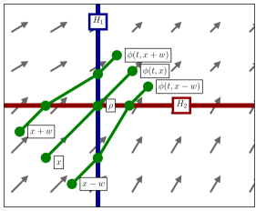
(a) $\dot{x}=F(x)$

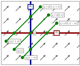
(b) $\dot{\widetilde{x}}=D\chi\circ F\circ\chi^{-1}(\widetilde{x})$

Figure 3: (a) Illustration of the vector field $F:\mathbb{R}^{2}\rightarrow T\mathbb{R}^{2}$ from (54) in the planar case $d=2$. (b) Pushforward of $F$ via the piecewise–linear (“flowbox”) homeomorphism $\chi:D\rightarrow D$ from (59).

7.1.3 Synchronization via piecewise–constant feedback

Now, returning to the state space of interest, let $U_{\Delta}\subset Q$ be the following open set parameterized by $\Delta>0$:

$$U_{\Delta}=\left\{q\in TQ\mid\exists x\in\pi^{-1}(q):\left\|x\right\|_{1}\leq\frac{\Delta}{d}\right\};$$ (65)

for $\Delta>0$ sufficiently small, $U_{\Delta}$ is “evenly covered” in the sense that $\pi|_{\pi^{-1}}(U_{\Delta})$ is a homeomorphism [Lee12, Appendix A]. Consider the effect of applying feedback of the form

$$\forall q\in Q:u(q)=\left\{\begin{array}[]{ll}-\delta\operatorname{sign}\circ\,\pi^{-1}(q),&q\in U;\\ 0,&q\in Q\setminus U;\end{array}\right.$$ (66)

to (52). It is straightforward to show (as we do in Appendix B.1) that the synchronized orbit $\Gamma$ defined in (53) is a periodic orbit for (52) under this feedback; we note that the closed–loop dynamics determine an event–selected $C^{\infty}$ vector field on a neighborhood of $\Gamma$.

Now we choose a local section $\Sigma\subset Q\setminus U_{\Delta}$ for the closed–loop dynamics that is perpendicular to $\Gamma$ and let $P\in PC^{\infty}(S,\Sigma)$ denote a Poincaré map for $\Gamma$ over a neighborhood $S\subset\Sigma$ containing $\left\{\rho\right\}=\Gamma\cap\Sigma$. To compute $DP(\rho)$ we employ (49), which involves solving the jump–linear time–varying differential equation (45) with the saltation matrix update given by (57). Note that away from discontinuities introduced by the feedback (66) the vector field in (52) does not depend on the state. This implies that $D_{x}F\equiv 0$, hence the continuous–time portion of the variational dynamics (45) does not alter the derivative computation.

Focusing our attention to the discrete–time (saltation matrix) portion of the variational dynamics (45), the closed–loop dynamics are discontinuous at three points in $\Gamma$: $\left\{-\Delta\mathds{1},0_{d},+\Delta\mathds{1}\right\}$. At $0_{d}$, the saltation matrix is given by (57). At $\pm\Delta\mathds{1}$, the update is determined by a single event surface that we chose to be perpendicular to $\Gamma$; although these updates affect $D\phi$, they have no effect on $DP$ since they lie in the kernel of $D\psi$ in (49). We conclude that $P$ is $C^{1}$ and

$$DP(\rho)=\frac{\nu-\delta}{\nu+\delta}I_{d-1}.$$ (67)

Therefore the induced norm contraction hypothesis of Proposition 2 (induced norm test for periodic orbit stability) is satisfied with the standard Euclidean norm and $c=\frac{\nu-\delta}{\nu+\delta}$. We conclude that $\Gamma$ is exponentially stable, whence the state feedback in (66) synchronizes the first–order phase oscillators in (52) at an exponential rate.

7.2 Synchronization of Second–Order Phase Oscillators

In this section we study synchronization in a system consisting of $d$ second–order phase oscillators, i.e. a control system of the form

$$\ddot{q}=\alpha\mathds{1}-\beta\dot{q}+u(q,\dot{q}),$$ (68)

where $q\in Q=\mathbb{R}^{d}/\mathbb{Z}^{d}$, $\alpha,\beta\in\mathbb{R}$ are constants, and $u:TQ\rightarrow T^{*}Q$ is a state–dependent feedback law. The state space is the tangent bundle $TQ$ of the $d$–dimension-al torus $Q=\mathbb{R}^{d}/\mathbb{Z}^{d}$; we let $\pi:\mathbb{R}^{2d}\rightarrow TQ$ denote the canonical quotient projection.

If $u\equiv\mu\mathds{1}$ where $\mu\in\mathbb{R}$ is a constant then (68) reduces to $d$ decoupled cascades of a pair of scalar affine time–invariant systems, thus it is clear that $\ddot{q}\rightarrow 0$ and hence $\dot{q}\rightarrow\frac{\alpha+\mu}{\beta}\mathds{1}$ as $t\rightarrow\infty$; this convergence is exponential with rate $\beta$. In this section, we propose a piecewise–constant form for the feedback $u$ and prove that for all $\beta$ sufficiently large there exists an exponentially stable periodic orbit that passes near $(0,\frac{\alpha}{\beta}\mathds{1})\in TQ$.

7.2.1 B–derivative of flow in Euclidean covering space

First, consider the vector field $F:\mathbb{R}^{2d}\rightarrow T\mathbb{R}^{2d}$ defined by

$$\forall(x,\dot{x})\in\mathbb{R}^{2d}:F(x,\dot{x})=\left[\begin{array}[]{c}\dot{x}\\ \alpha\mathds{1}-\beta\dot{x}-\delta\operatorname{sign}(x)\end{array}\right]$$ (69)

where $0<\delta<\alpha$ is a given constant. Clearly $F$ is event–selected $C^{\infty}$ on the open set

$$D=\left\{(x,\dot{x})\in\mathbb{R}^{2d}\mid\forall j\in\left\{1,\dots,d\right\}:\dot{x}_{j}\neq 0\right\}\subset\mathbb{R}^{2d}$$ (70)

since the event surfaces coincide with the first $d$ standard coordinate planes in $\mathbb{R}^{2d}$; since $F$ fails to be event–selected $C^{r}$ at points with zero velocity, we exclude them from our analysis. Let $\phi:\mathscr{F}\rightarrow D$ denote the global flow for $F$ yielded by Corollary 1.

We begin by computing the B–derivative of the flow with respect to state along the trajectory passing through a point $(0,\nu\mathds{1})\in D$ where $\nu>0$. For clarity we outline the computation here and relegate a detailed derivation to Appendix B.2. For any word $\omega\in\Omega$ we can obtain the derivative of the selection function $\phi_{\omega}$ with respect to state from (46),

$$D_{x}\phi_{\omega}(0,(0,\nu\mathds{1}))=F(\phi(0,x))\Lambda^{\top}_{\omega}(0)+X_{\omega}(0)=\Xi_{\omega}\left[\begin{array}[]{c}0_{2d}^{\top}\\ I_{2d}\end{array}\right],$$ (71)

since $\Lambda^{\top}_{\omega}(0)=0_{2d}^{\top}$ and $X_{\omega}(0)=I_{2d}$. The saltation matrix $\Xi_{\omega}$, given in general by (41), simplifies in this example to (109), whence we conclude as in (113) that

$$D_{x}\phi_{\omega}(0,(0,\nu\mathds{1}))=\left[\begin{array}[]{cc}I_{d}&0\\ -\frac{2\delta}{\nu}I_{d}&I_{d}\end{array}\right].$$ (72)

This shows that $\phi$ is in fact $C^{1}$ with respect to state at $(0,(0,\nu\mathds{1}))\in\mathscr{F}$, and hence

$$\forall(p,\dot{p})\in T_{(0,\nu\mathds{1})}D:D\phi(0,(0,\nu\mathds{1});0,(p,\dot{p}))=\left[\begin{array}[]{cc}I_{d}&0\\ -\frac{2\delta}{\nu}I_{d}&I_{d}\end{array}\right]\left[\begin{array}[]{c}p\\ \dot{p}\end{array}\right]=:\Xi\left[\begin{array}[]{c}p\\ \dot{p}\end{array}\right],$$ (73)

i.e. the first–order effect of the nonsmooth flow associated with this piecewise–constant vector field is a change in velocity $\dot{p}\mapsto\dot{p}-\frac{2\delta}{\nu}p$ that is proportional to the error in position $p$. Solving the variational equation as in Section 6.1, a straightforward calculation (given for completeness in Appendix B.2) yields

$$\left[\begin{array}[]{c}p(s)\\ \dot{p}(s)\end{array}\right]=\left[\begin{array}[]{cc}I_{d}&\frac{1}{\beta}\left(1-e^{-\beta s}\right)I_{d}\\ 0&e^{-\beta s}I_{d}\end{array}\right]\left[\begin{array}[]{c}p(0^{+})\\ \dot{p}(0^{+})\end{array}\right]=:X(s)\left[\begin{array}[]{c}p(0^{+})\\ \dot{p}(0^{+})\end{array}\right],$$ (74)

where $(p(0^{+}),\dot{p}(0^{+}))$ is determined from $(p(0),\dot{p}(0))\in T_{(0,\nu\mathds{1})}D$ by applying (73). Combining (73) with (74) we conclude that the B–derivative with respect to state at time $s$ is given by

$$\left[\begin{array}[]{c}p(s)\\ \dot{p}(s)\end{array}\right] =D\phi\left(s,\left[\begin{array}[]{c}x(0)\\ \dot{x}(0)\end{array}\right];0,\left[\begin{array}[]{c}p(0)\\ \dot{p}(0)\end{array}\right]\right)$$ (75)

$$=X(s)\ \Xi\left[\begin{array}[]{c}p(0)\\ \dot{p}(0)\end{array}\right]$$

$$=\left[\begin{array}[]{cc}I_{d}&\frac{1}{\beta}\left(1-e^{-\beta s}\right)I_{d}\\ 0&e^{-\beta s}I_{d}\end{array}\right]\left[\begin{array}[]{cc}I_{d}&0\\ -\frac{2\delta}{\nu}I_{d}&I_{d}\end{array}\right]\left[\begin{array}[]{c}p(0)\\ \dot{p}(0)\end{array}\right]$$

$$=\left[\begin{array}[]{cc}I_{d}-\frac{2\delta}{\beta\nu}\left(1-e^{-\beta s}\right)I_{d}&\frac{1}{\beta}\left(1-e^{-\beta s}\right)\\ -\frac{2\delta}{\nu}e^{-\beta s}I_{d}&e^{-\beta s}I_{d}\end{array}\right]\left[\begin{array}[]{c}p(0)\\ \dot{p}(0)\end{array}\right].$$

Taking the limit as $s\rightarrow\infty$,

$$\left[\begin{array}[]{c}p(\infty)\\ \dot{p}(\infty)\end{array}\right]=\lim_{s\rightarrow\infty}\left[\begin{array}[]{c}p(s)\\ \dot{p}(s)\end{array}\right]=\left[\begin{array}[]{c}\left(1-\frac{2\delta}{\beta\nu}\right)p(0)\\ 0\end{array}\right].$$ (76)

In plain language (76) indicates that, to first order, the nonsmooth flow associated with the vector field (69) asymptotically (i) drives the initial velocity error $\dot{p}(0)$ to zero and (ii) multiplies the initial position error $p(0)$ by a factor of $c=\left(1-\frac{2\delta}{\beta\nu}\right)$. If we ensure $\nu\in\left(\frac{\alpha}{\beta},\frac{\alpha+\delta}{\beta}\right)$, then $c=\left(1-\frac{2\delta}{\beta\nu}\right)\in\left(1-\frac{2\delta}{\alpha},1-\frac{2\delta}{\alpha+\delta}\right)\subset(-1,+1)$, achieving contraction in positions. Finally, we note that the convergence in (76) is exponential with rate $\beta$.

7.2.2 Synchronization via piecewise–constant feedback

We now apply a construction analogous to that of Section 7.1 to define a piecewise–constant feedback law that results in an exponentially stable periodic orbit that passes near $(0,\frac{\alpha}{\beta}\mathds{1})\in TQ$. To that end, consider the following form for the control neighborhood $U_{\Delta}\subset TQ$ parameterized by $\Delta>0$:

$$U_{\Delta}=\left\{\vphantom{\int}(q,\dot{q})\in TQ\mid\right. \left(\exists(x,\dot{x})\in\pi^{-1}(q,\dot{q}):\left\|x\right\|_{1}\leq\frac{\Delta}{d}\right)$$ (77)

$$\left.\vphantom{\int}\wedge\left(\forall j\in\left\{1,\dots,d\right\}:\dot{q}_{j}>0\right)\right\};$$

for $\Delta>0$ sufficiently small, $U_{\Delta}$ is “evenly covered” in the sense that $\pi|_{\pi^{-1}}(U_{\Delta})$ is a homeomorphism [Lee12, Appendix A]. Furthermore, “synchronized” points of the form $(\pm\Delta\mathds{1},\nu\mathds{1})$ where $\nu>0$ are in the boundary $\partial U_{\Delta}$. We study the effect of applying feedback of the form

$$\forall(q,\dot{q})\in TQ:u(q,\dot{q})=\left\{\begin{array}[]{ll}-\delta\operatorname{sign}\circ\,\pi^{-1}(q,\dot{q}),&(q,\dot{q})\in U_{\Delta};\\ 0,&(q,\dot{q})\in TQ\setminus U_{\Delta};\end{array}\right.$$ (78)

to (68). It is straightforward to show (as we do in Appendix B.2) that for all $\beta>0$ sufficiently large there exists $\nu_{\beta}\in\left(\frac{\alpha}{\beta},\frac{\alpha+\delta}{\beta}\right)$ such that the trajectory initialized at $(0,\nu_{\beta}\mathds{1})$ is periodic for the dynamics in (68) subject to the piecewise–constant forcing (78). We let $\Gamma_{\beta}\subset TQ$ denote the image of the periodic orbit, and let $\nu_{\beta}^{-}$ (resp. $\nu_{\beta}^{+}>0$) denote the speed of the orbit when the position is equal to $-\Delta\mathds{1}$ (resp. $+\Delta\mathds{1}$) so that $(-\Delta\mathds{1},\nu_{\beta}^{-}\mathds{1})\in\Gamma_{\beta}$ (resp. $(+\Delta\mathds{1},\nu_{\beta}^{+}\mathds{1})\in\Gamma_{\beta}$). Note that, by increasing $\beta$, $\nu_{\beta}^{-}$ can be made arbitrarily close to $\frac{\alpha}{\beta}$ and $\nu_{\beta}$ can be made arbitrarily close to $\frac{\alpha+\delta}{\beta}$, whence $\nu_{\beta}\in\left(\frac{\alpha}{\beta},\frac{\alpha+\delta}{\beta}\right)$. Further, note that the closed–loop dynamics determine an event–selected $C^{\infty}$ vector field on a neighborhood of $\Gamma_{\beta}$.

Now we choose a local section $\Sigma_{\beta}\subset TQ\setminus U_{\Delta}$ for the closed–loop dynamics whose normal vector is parallel to $(\mathds{1},0)$ at the point $\rho_{\beta}=(-\Delta\mathds{1},\nu_{\beta}^{-}\mathds{1})\in\Gamma_{\beta}\cap\Sigma_{\beta}$. Note that by construction $\Sigma_{\beta}\cap\partial U_{\Delta}$ is an open set containing $\rho_{\beta}$. Let $P_{\beta}\in PC^{\infty}(S_{\beta},\Sigma_{\beta})$ denote a Poincaré map for $\Gamma_{\beta}$ over a neighborhood $S_{\beta}\subset\Sigma_{\beta}$ containing $\left\{\rho_{\beta}\right\}$. To compute $DP_{\beta}(\rho_{\beta})$ we employ (49), which involves solving the jump–linear time–varying differential equation (45) with the saltation matrix update given by (73). Away from discontinuities introduced by the feedback (78) the state dependence of the vector field in (68) is confined to viscous drag on velocities. This implies that the continuous–time portion of the variational dynamics (45) is given by (74), i.e. the first–order effect of the flow contracts velocity error at an exponential rate and amplfies position error by an amount proportional to $1/\beta$.

Focusing our attention now on the discrete–time (saltation matrix) portion of the variational dynamics (45), the closed–loop dynamics are discontinuous at three points in $\Gamma$: $(-\Delta\mathds{1},\nu_{\beta}^{-}\mathds{1})$, $(0,\nu\mathds{1})$, and $(+\Delta\mathds{1},\nu_{\beta}^{+}\mathds{1})$. At $(0,\nu\mathds{1})$, the saltation matrix is given by (73). At $(\pm\Delta\mathds{1},\nu_{\beta}^{\pm})$, the saltation matrix is determined by a single event surface whose normal vector is parallel to $(\mathds{1},0)$. Although these updates affect $D\phi$, they have no effect on $DP_{\beta}$ since they lie in the kernel of $D\psi$ in (49). We conclude that $P_{\beta}$ is $C^{1}$ and

$$DP_{\beta}(\rho_{\beta})=\left[\begin{array}[]{cc}\left(1-\frac{2\delta}{\beta\nu_{\beta}}\right)I_{d-1}&0\\ 0&0\end{array}\right]+E_{\beta}$$ (79)

where the induced norm of the error term $\left\|E_{\beta}\right\|_{i}$ decreases exponentially with increasing $\beta$. Therefore for all $\beta>0$ sufficiently large the induced norm contraction hypothesis of Proposition 2 (induced norm test for periodic orbit stability) is satisfied with the standard Euclidean norm and $c\approx\left(1-\frac{2\delta}{\beta\nu_{\beta}}\right)\in\left(1-\frac{2\delta}{\alpha},1-\frac{2\delta}{\alpha+\delta}\right)\subset(-1,+1)$. We conclude that $\Gamma_{\beta}$ is exponentially stable for all $\beta>0$ sufficiently large, whence the state feedback in (78) synchronizes the second–order phase oscillators in (68) at an exponential rate.

8 Discussion

In this paper, we studied local properties of the flow generated by vector fields with “event–selected” discontinuities, that is, vector fields that are (i) smooth except along a finite collection of smooth submanifolds and (ii) “transverse” to these submanifolds in the sense that integral curves intersect them at isolated points in time. We emphasize that the vector field transversality condition (ii) excludes sliding modes [Utk77, Jef14] from our analysis. Basic properties of discontinuous vector fields have been studied in a more general setting, for instance yielding sufficient conditions ensuring existence of a continuous flow (see [Fil88, Chapter 2] generally and [Fil88, Theorem 3 in §8] specifically). Our chief contribution is the introduction of techniques from non–smooth analysis [Sch12] to show that a vector field with event–selected discontinuities yields a continuous flow that admits a strong first–order approximation, the (so–called [Rob87]) Bouligand derivative. We employed this B–derivative to obtain fundamental constructions familiar from classical (smooth) dynamical systems theory, including impact maps, flowboxes, and variational equations, and to study the effect of perturbations, both infinitesimal and non–infinitesimal. In the classical setting, these constructions are obtained using the classical (alternately called Fréchet [Sch12, Section 3.1] or Jacobian [GH83, Section 1.3]) derivative of the smooth flow; our construction of the non–smooth object proceeded analogously to that of its smooth counterpart after replacing the classical derivative of the flow with our B–derivative. Thus the piecewise–differentiable dynamical systems we study bear a closer resemblance to classically differentiable dynamical systems than to discontinuous dynamical systems considered, for instance, in [PB10, Jim+13].

In future work, we expect to obtain generalizations of other techniques from the classical theories of dynamical and control systems that depend primarily on the existence of first– or higher–order approximations of the flow, for instance: stability analysis via control Lyapunov functions [Art83, Son89] or infinitesimal contractivity [LS98, Son10]; conditions for controllability based on the inverse function theorem [LN93, Theorem 8] [Car+09, Section II.C]; or necessary and sufficient conditions for optimality in nonlinear programs involving dynamical systems [Pol97, Chapter 4]. More broadly, we believe our results support the study of a class of discontinuous vector fields that arise in neuroscience [Kee+81], biological and robotic locomotion [Hol+06], and electrical engineering [His95]. In each of these disparate domains, behaviors of interest occur near the intersection of surfaces of discontinuity, hence the techniques we developed in this paper may be brought to bear. Thus we conclude with brief remarks about the formal applicability and practical relevance of our results in these applications.

Integrate–and–fire neuron models consist of a population of $n$ subsystems that undergo a discontinuous change in membrane voltage triggered by crossing a voltage threshold [Kee+81],

$$\dot{v} =-\gamma v+u,$$ (80)

$$v(t^{+}) =0\ \text{if}\ v(t^{-})=\overline{v},$$

where: $v\in\mathbb{R}$ is the membrane voltage; $\gamma\in\mathbb{R}$ is a dissipation constant; $u\in\mathbb{R}$ is an exogenous input; and $\overline{v}\in\mathbb{R}$ is the firing threshold. When driven by a periodic exogenous input, integrate–and–fire neuron populations can exhibit phase locking [Kee+81] or local synchronization [HH95] behavior, resulting in simultaneous or near–simultaneous firing. Of interest in applications is the computation of so–called “Lyapunov exponents” using variational equations. We showed in Section 6.1 that the variational equation must be supplemented by discontinuous updates via saltation matrices near such simultaneous–firing events. As noted in [Biz+13, Section 4.1], neglecting this non–smooth effect can result in erroneous conclusions.

Legged locomotion of animals and robots involves intermittent interaction of limbs with terrain; their dynamics are given by [Joh+, Section II],

$$M(q)\ddot{q} =f(q,\dot{q})+\lambda(q,\dot{q})Da(q),$$ (81)

$$\dot{q}(t^{+}) =R(q(t))\dot{q}(t^{-})\ \text{if}\ a_{j}(t^{-})=0,$$

where: $q\in Q$ is a vector of generalized coordinates for the body and limbs; $M$ is the inertia tensor; $f:TQ\rightarrow T^{*}Q$ contains internal, applied, and Coriolis forces; $a:Q\rightarrow\mathbb{R}^{n}$ specifies $n$ unilateral constraints of the form

$$\forall j\in\left\{1,\dots,n\right\}:a_{j}(q)\geq 0;$$ (82)

$\lambda:TQ\rightarrow T^{*}Q$ denotes the reaction forces that ensure (82) are satisfied by (81) for all time. The update $\dot{q}(t^{+})=R(q(t))\dot{q}(t^{-})$ is triggered when one of the unilateral constraints $a_{j}$ would be violated by a penetrating velocity; it causes a discontinuity in both the velocity and the forces acting on the system. Legged animals and robots with four, six, and more limbs exhibit gaits with near–simultaneous touchdown of two or more legs [Ale84, Gol+99, Hol+06]. Steady–state gaits are commonly modeled as periodic orbits in the body reference frame [SK88, KB91, KF99]. In practice, gait stability is assessed using the linearization of the first–return or Poincaré map, since if the eigenvalues of the linearization (the so–called Floquet multipliers [GH83, Section 1.5]) lie within the unit disk then the gait is exponentially stable [AG58, Gri+02]. We showed in Section 4.2 that the Poincaré map associated with a periodic orbit passing through the intersection of multiple surfaces of discontinuity is generally non–smooth. This implies that it is not possible to assess stability of such orbits using the F–derivative since the F–derivative of the map does not exist. In Section 6.2, we showed how the B–derivative of the Poincaré map can be employed instead to assess stability of such orbits.

Electrical power systems undergo discontinuous changes in network topology triggered by excessive voltages or currents, leading to differential–algebraic models of the form [His95, (2)–(4)]

$$\dot{x} =f(x,y,z;p),\ 0=g(x,y,z;p),$$ (83)

$$z(t^{+}) =h(x(t),y(t),z(t^{-});p)\ \text{if}\ y_{j}(t^{-})=0,$$

where: $x\in\mathbb{R}^{d}$ contains dynamic states; $y\in\mathbb{R}^{n}$ contains algebraic states; $z\in\mathbb{R}^{m}$ contains discrete states; $p\in\mathbb{R}^{\ell}$ contains parameters; $f:\mathbb{R}^{d+n+m+\ell}\rightarrow\mathbb{R}^{d}$ is a smooth vector field; $g:\mathbb{R}^{d+n+m+\ell}\rightarrow\mathbb{R}^{k}$ is a smooth constraint function; and $h:\mathbb{R}^{d+n+m+\ell}\rightarrow\mathbb{R}^{m}$ is a smooth reset function. The update $z(t^{+})=h(x(t),y(t),z(t^{-});p)$ is applied when one of the algebraic states $y_{j}$ crosses a prespecified threshold (e.g. a bus voltage limit), causing a discontinuity in the vector field governing the time evolution of $x$. In electrical power networks, discrete switches triggered by over–excitation limits can occur at arbitrary times with respect to one another. When the switches occur at distinct time instants, the trajectory sensitivity matrix (i.e. the F–derivative the flow) computed as in [HP00] can provide quantitative insights for design and control. However, as noted in [HP00, Section VIII], these calculations lose accuracy when event times become coincident; this is due to the fact that the flow is not classically differentiable along trajectories that undergo simultaneous discrete transitions. The procedure we developed in Section 6.1 can be employed to compute a collection of trajectory sensitivity matrices (i.e. the B–derivative of the flow) that generalize the approach advocated in [HP00] to be applicable in power networks that undergo an arbitrary (but finite) number of simultaneous discrete transitions.

Support

This research was supported in part by: an NSF Graduate Research Fellowship to S. A. Burden; ARO Young Investigator Award #61770 to S. Revzen; ARL Cooperative Agreements W911NF–08–2–0004 and W911NF–10–2–0016; and NSF Award #1028237. The views and conclusions contained in this document are those of the authors and should not be interpreted as representing the official policies, either expressed or implied, of the Army Research Laboratory or the U.S. Government. The U.S. Government is authorized to reproduce and distribute for Government purposes notwithstanding any copyright notation herein.

Appendix A F–Derivative Formulae for Piecewise–Differentiable Flow

A piecewise–differentiable function is differentiable almost everywhere [Roc03, Theorem 2], and hence its B–derivative at any point is contained in the convex hull of the limit of F–derivatives of its selection functions [Sch12, § 4.3]. For completeness and to aid the reader’s comprehension, we now derive explicit formulae for F–derivatives of the piecewise–differentiable objects used in Section 3.3 to construct the piecewise–differentiable flow. In general the B–derivative can be obtained via the chain rule [Sch12, Theorem 3.1.1].

A.1 Budgeted time–to–boundary

We adopt the notational conventions from Section 3.2.1.

Define $\nu_{b}^{+}:U_{b}\rightarrow\mathbb{R}\cup\left\{+\infty\right\}$ using the convention $\min\emptyset=+\infty$ by

$$\forall x\in U_{b}:\nu_{b}^{+}(x)=\min\left\{\tau_{b}^{H_{j}}(x):b_{j}<0\right\}_{j=1}^{n},$$ (84)

then for all $(t,x)\in\mathbb{R}\times U_{b}$ such that $\nu_{b}^{+}(x)\neq t\neq 0$, the forward–time budgeted time–to–boundary $\tau_{b}^{+}$ is classically differentiable and

$$D\tau_{b}^{+}(t,x)=\left\{\begin{array}[]{ll}(0,\ 0_{d}^{\top}),&t<0;\\ (1,\ 0_{d}^{\top}),&0<t<\nu_{b}^{+}(x);\\ \left(0,D\tau_{b}^{H}(x)\right),&\nu_{b}^{+}(x)<t;\end{array}\right.$$ (85)

where in the third case $H\in\left\{H_{j}\right\}_{j=1}^{n}$ is such that $\tau_{b}^{H}(x)=\nu_{b}^{+}(x)>0$.

Define $\nu_{b}^{-}:U_{b}\rightarrow\mathbb{R}\cup\left\{-\infty\right\}$ using the convention $\max\emptyset=-\infty$ by

$$\forall x\in U_{b}:\nu_{b}^{-}(x)=\min\left\{\tau_{b}^{H_{j}}(x):b_{j}>0\right\}_{j=1}^{n},$$ (86)

then for all $(t,x)\in\mathbb{R}\times U_{b}$ such that $\nu_{b}^{-}(x)\neq t\neq 0$, the backward–time budgeted time–to–boundary $\tau_{b}^{-}$ is classically differentiable and

$$D\tau_{b}^{-}(t,x)=\left\{\begin{array}[]{ll}(0,\ 0_{d}^{\top}),&t>0;\\ (1,\ 0_{d}^{\top}),&\nu_{b}^{-}(x)<t<0;\\ \left(0,D\tau_{b}^{H}(x)\right),&t<\nu_{b}^{-}(x);\end{array}\right.$$ (87)

where in the third case $H\in\left\{H_{j}\right\}_{j=1}^{n}$ is such that $\tau_{b}^{H}(x)=\nu_{b}^{-}(x)<0$.

A.2 Budgeted flow–to–boundary

We adopt the notational conventions from Section 3.2.2.

Define $\nu_{b}^{+}:U_{b}\rightarrow\mathbb{R}$ as in (84) then for all $(t,x)\in\mathbb{R}\times U_{b}$ such that $\nu_{b}^{+}(x)\neq t\neq 0$, the forward–time flow–to–boundary $\zeta_{b}^{+}$ is classically differentiable and

$$D\zeta_{b}^{+}(t,x)=\left\{\begin{array}[]{ll}(0_{d},\ 0_{d\times d}),&t<0;\\ (F_{b}(\phi_{b}(t,x)),\ D_{x}\phi_{b}(t,x)),&0<t<\nu_{b}^{+}(x);\\ (0_{d},\Upsilon(t,x)),&\nu_{b}^{+}(x)<t;\end{array}\right.$$ (88)

where in the third case $\Upsilon(t,x)=F_{b}(\phi_{b}(\tau_{b}^{+}(t,x),x))D\tau_{b}^{H}(x)+D_{x}\phi_{b}(\tau_{b}^{+}(t,x),x)$ and $H\in\left\{H_{j}\right\}_{j=1}^{n}$ is such that $\tau_{b}^{H}(x)=\nu_{b}^{+}(x)$.

Define $\nu_{b}^{-}:U_{b}\rightarrow\mathbb{R}$ as in (86) then for all $(t,x)\in\mathbb{R}\times U_{b}$ such that $\nu_{b}^{-}(x)\neq t\neq 0$, the backward–time flow–to–boundary $\zeta_{b}^{-}$ is classically differentiable and

$$D\zeta_{b}^{-}(t,x)=\left\{\begin{array}[]{ll}(0_{d},\ 0_{d\times d}),&t>0;\\ (F_{b}(\phi_{b}(t,x)),\ D_{x}\phi_{b}(t,x)),&\nu_{b}^{-}(x)<t<0;\\ \left(0_{d},\Upsilon(t,x)\right),&t<\nu_{b}^{-}(x);\end{array}\right.$$ (89)

where in the third case $\Upsilon(t,x)=F_{b}(\phi_{b}(\tau_{b}^{-}(t,x),x))D\tau_{b}^{H}(x)+D_{x}\phi_{b}(\tau_{b}^{-}(t,x),x)$ and $H\in\left\{H_{j}\right\}_{j=1}^{n}$ is such that $\tau_{b}^{H}(x)=\nu_{b}^{+}(x)$.

A.3 Composite of budgeted time–to– and flow–to–boundary

We adopt the notational conventions from Section 3.2.3.

Combine (6) and (8) to obtain the derivative of $\varphi_{b}^{+}$ for all $(t,x)\in\mathbb{R}\times U_{b}$ such that $\nu_{b}^{+}(x)\neq t\neq 0$:

$$D\varphi_{b}^{+}(t,x)=\left\{\begin{array}[]{ll}\left[\begin{array}[]{cc}1&0\\ 0&I\end{array}\right],&t<0;\\ \left[\begin{array}[]{cc}0&0\\ F_{b}(\phi_{b}(t,x))&D_{x}\phi_{b}(t,x)\end{array}\right],&0<t<\nu_{b}^{+}(x);\\ \left[\begin{array}[]{cc}1&-D\tau_{b}^{H}(x)\\ 0&\Upsilon(t,x)\end{array}\right],&\nu_{b}^{+}(x)<t;\end{array}\right.$$ (90)

where in the third case $\Upsilon(t,x)=F_{b}(\phi_{b}(\tau_{b}^{+}(t,x),x))D\tau_{b}^{H}(x)+D_{x}\phi_{b}(\tau_{b}^{+}(t,x),x)$ and $H\in\left\{H_{j}\right\}_{j=1}^{n}$ is such that $\tau_{b}^{H}(x)=\nu_{b}^{+}(x)$.

Combine (87) and (89) to obtain the derivative of $\varphi_{b}^{-}$ for all $(t,x)\in\mathbb{R}\times U_{b}$ such that $\nu_{b}^{-}(x)\neq t\neq 0$:

$$D\varphi_{b}^{-}(t,x)=\left\{\begin{array}[]{ll}\left[\begin{array}[]{cc}1&0\\ 0&I\end{array}\right],&t>0;\\ \left[\begin{array}[]{cc}0&0\\ F_{b}(\phi_{b}(t,x))&D_{x}\phi_{b}(t,x)\end{array}\right],&\nu_{b}^{-}(x)<t<0;\\ \left[\begin{array}[]{cc}1&-D\tau_{b}^{H}(x)\\ 0&\Upsilon(t,x)\end{array}\right],&t<\nu_{b}^{-}(x);\end{array}\right.$$ (91)

where in the third case $\Upsilon(t,x)=F_{b}(\phi_{b}(\tau_{b}^{-}(t,x),x))D\tau_{b}^{H}(x)+D_{x}\phi_{b}(\tau_{b}^{-}(t,x),x)$ and $H\in\left\{H_{j}\right\}_{j=1}^{n}$ is such that $\tau_{b}^{H}(x)=\nu_{b}^{+}(x)$.

Appendix B Periodic Orbits and B–derivative Formulae for Phase Oscillators

In the following subsections we provide detailed derivations that were deemed too laborious to include in the main text.

B.1 Synchronization of First–Order Phase Oscillators

We adopt the notational conventions of Section 7.1, and derive several useful properties of closed–loop dynamics obtained by applying the piecewise–constant feedback in (66) to the system in (52).

First we argue that the synchronized set (53) is a periodic orbit for the closed–loop dynamics. Since (52) consists of $d$ identical subsystems and the feedback in (66) encounters discontinuities synchronously (i.e. all coordinates of the vector field change discontinuously at the same time) at points $\left\{-\Delta\mathds{1},0_{d},+\Delta\mathds{1}\right\}$ and at every other point in time the vector field coordinates are identical, we conclude that the trajectory initialized at $0_{d}$ remains synchronized for all time.

We now explicitly derive the B–derivative in (57). Fixing a word $\omega:\left\{1,\dots,d\right\}\rightarrow B_{d}$ with corresponding sequence of surfaces crossed $\eta:\left\{1,\dots,d\right\}\rightarrow\left\{1,\dots,d\right\}$, we know from Section 6.1 that for all $\varepsilon>0$ the F–derivative of the selection function $\phi_{\omega}$ at $(2\varepsilon,\phi(-\varepsilon,0_{d}))$ is given by (39),

$$D\phi_{\omega}(2\varepsilon,\phi(-\varepsilon,0_{d}))=D\phi(\varepsilon,0_{d})\left[\prod_{j=1}^{d}D\varphi_{\omega(j)}^{+}(0,0_{d})\right]\left[\begin{array}[]{c}0\\ D\phi(\varepsilon,\phi(-\varepsilon,0_{d}))\end{array}\right].$$ (92)

Here, $D\phi(\varepsilon,0_{d})$, $D\phi(\varepsilon,\phi(-\varepsilon,0_{d}))$ are obtained as in (33) by solving the classical variational equation since $F:\mathbb{R}^{d}\rightarrow T\mathbb{R}^{d}$ is smoothly extendable to a neighborhood of those segments of the trajectory; noting that for all $s\in[-\varepsilon,0)$ we have $F(\phi(s,0_{d}))=F_{-\mathds{1}}(0_{d})$, $D_{x}F(\phi(s,0_{d}))=0$ and for all $s\in(0,+\varepsilon]$ we have $F(\phi(s,0_{d}))=F_{+\mathds{1}}(0_{d})$, $D_{x}F(\phi(s,0_{d}))=0$, we conclude that

$$D\phi(s,0_{d})=\left[\begin{array}[]{cc}F_{+\mathds{1}}(0_{d})&I_{d}\end{array}\right],\ D\phi(s,\phi(-s,0_{d}))=\left[\begin{array}[]{cc}F_{-\mathds{1}}(0_{d})&I_{d}\end{array}\right].$$ (93)

For each $j\in\left\{1,\dots,d\right\}$ the derivative $D\varphi_{\omega(j)}^{+}(0,0_{d})$ is given by the matrix in the third case in (11) with the simplifications $\tau_{\omega(j)}^{+}(0,0_{d})=0$, $\phi_{\omega(j)}(0,0_{d})=0_{d}$; setting $f_{j}=F_{\omega(j)}(0_{d})$, $g_{j}^{\top}=Dh_{\eta(j)(0_{d})}$ for each $j\in\left\{1,\dots,d\right\}$, by (40) we have

$$D\varphi_{\omega(j)}^{+}(0,0_{d})=I_{d+1}+\frac{1}{g_{j}^{\top}f_{j}}\left[\begin{array}[]{c}1\\ -f_{j}\end{array}\right]\left[\begin{array}[]{cc}0&g_{j}^{\top}\end{array}\right].$$ (94)

Now for all $j\in\left\{1,\dots,d\right\}$ we have $f_{j}=F_{\omega(j)}(0_{d})=\nu\mathds{1}-\delta\omega(j)\in\mathbb{R}^{d}$ and $g_{j}^{\top}=Dh_{\eta(j)}(0_{d})=e_{\eta(j)}^{\top}\in\mathbb{R}^{1\times d}$, hence $g_{j}^{\top}f_{j}=\nu+\delta$. Since for all $i\in\left\{1,\dots,d\right\}$ with $i>j$ the vector $\omega(i)$ is lexicographically greater than $\omega(j)$, we also have $g_{i}^{\top}f_{j}=\nu+\delta$. These simplifications yield for all $j\in\left\{1,\dots,d-1\right\}$

$$D \varphi_{\omega(j+1)}^{+}(0,0_{d})D\varphi_{\omega(j)}^{+}(0,0_{d})$$ (95)

$$=\left[I_{d+1}+\frac{1}{\nu+\delta}\left[\begin{array}[]{c}1\\ -f_{j+1}\end{array}\right]\left[\begin{array}[]{cc}0&e_{\eta(j+1)}^{\top}\end{array}\right]\right]\left[I_{d+1}+\frac{1}{\nu+\delta}\left[\begin{array}[]{c}1\\ -f_{j}\end{array}\right]\left[\begin{array}[]{cc}0&e_{\eta(j)}^{\top}\end{array}\right]\right]$$

$$=I_{d+1}+\frac{1}{\nu+\delta}\left[\begin{array}[]{c}1\\ -f_{j+1}\end{array}\right]\left[\begin{array}[]{cc}0&e_{\eta(j+1)}^{\top}\end{array}\right]+\frac{1}{\nu+\delta}\left[\begin{array}[]{c}0\\ f_{j+1}-f_{j}\end{array}\right]\left[\begin{array}[]{cc}0&e_{\eta(j)}^{\top}\end{array}\right].$$

Noting that $f_{j+1}-f_{j}=-2\delta e_{\eta(j)}$, we conclude that $e_{\eta(i)}^{\top}(f_{j+1}-f_{j})=0$ for all $i\in\left\{j+1,\dots,d\right\}$. This implies that

$$\Xi_{\omega} =\prod_{j=1}^{d}D\varphi_{\omega(j)}^{+}(0,0_{d})$$ (96)

$$=I_{d+1}+\frac{1}{\nu+\delta}\left[\begin{array}[]{c}1\\ -f_{d}\end{array}\right]\left[\begin{array}[]{cc}0&e_{\eta(d)}^{\top}\end{array}\right]+\frac{1}{\nu+\delta}\sum_{j=1}^{d-1}\left[\begin{array}[]{c}0\\ -2\delta e_{\eta(j)}\end{array}\right]\left[\begin{array}[]{cc}0&e_{\eta(j)}^{\top}\end{array}\right].$$

Noting for any $f\in\mathbb{R}^{d}$ with $0_{d}=0\cdot\mathds{1}_{d}\in\mathbb{R}^{d}$ that

$$\left[\begin{array}[]{cc}0&0_{d}^{\top}\\ f&I_{d}\end{array}\right]=I_{d+1}+\left[\begin{array}[]{c}-1\\ f\end{array}\right]\left[\begin{array}[]{cc}1&0_{d}^{\top}\end{array}\right],$$ (97)

defining $f^{+}=F_{+\mathds{1}}(0_{d})$ and noting that $f^{+}-f_{d}=-2\delta e_{\eta(d)}$ we have

$$\left[\begin{array}[]{cc}0&0_{d}^{\top}\\ f^{+}&I_{d}\end{array}\right]\prod_{j=1}^{d}D\varphi_{\omega(j)}^{+}(0,0_{d})= \,I_{d+1}+\left[\begin{array}[]{c}-1\\ f^{+}\end{array}\right]\left[\begin{array}[]{cc}1&0_{d}^{\top}\end{array}\right]$$ (98)

$$+\frac{1}{\nu+\delta}\left[\begin{array}[]{c}0\\ f^{+}-f_{d}\end{array}\right]\left[\begin{array}[]{cc}0&e_{\eta(d)}^{\top}\end{array}\right]$$

$$+\frac{1}{\nu+\delta}\sum_{j=1}^{d-1}\left[\begin{array}[]{c}0\\ -2\delta e_{\eta(j)}\end{array}\right]\left[\begin{array}[]{cc}0&e_{\eta(j)}^{\top}\end{array}\right]$$

$$= \,I_{d+1}-\frac{2\delta}{\nu+\delta}\left[\begin{array}[]{cc}0&0_{d}^{\top}\\ 0_{d}&I_{d}\end{array}\right]+\left[\begin{array}[]{c}-1\\ f^{+}\end{array}\right]\left[\begin{array}[]{cc}1&0_{d}^{\top}\end{array}\right].$$

Finally, defining $f^{-}=F_{-\mathds{1}}(0_{d})$ we have

$$D\phi_{\omega}(0,0_{d}) =\left[\begin{array}[]{cc}0&0_{d}^{\top}\\ f^{+}&I_{d}\end{array}\right]\prod_{j=1}^{d}D\varphi_{\omega(j)}^{+}(0,0_{d})\left[\begin{array}[]{cc}0&0_{d}^{\top}\\ f^{-}&I_{d}\end{array}\right]$$ (99)

$$=I_{d+1}-\frac{2\delta}{\nu+\delta}\left[\begin{array}[]{cc}0&0_{d}^{\top}\\ 0_{d}&I_{d}\end{array}\right]+\left[\begin{array}[]{c}-1\\ \left(\frac{\nu-\delta}{\nu+\delta}\right)f^{-}\end{array}\right]\left[\begin{array}[]{cc}1&0_{d}^{\top}\end{array}\right]$$

$$=\left[\begin{array}[]{cc}\left(\frac{\nu-\delta}{\nu+\delta}\right)f^{-}&\frac{\nu-\delta}{\nu+\delta}I_{d}\end{array}\right].$$

Restricting to the derivative with respect to state, we find for all words $\omega\in\Omega$ that

$$D_{x}\phi_{\omega}(0,0_{d})=\frac{\nu-\delta}{\nu+\delta}I_{d}.$$ (100)

Thus the piecewise–differentiable flow $\phi$ is $C^{1}$ with respect to state at $(0,0_{d})$, and (57) follows. Restricting instead to the derivative with respect to time, we find as expected that

$$D_{t}\phi_{\omega}(0,0_{d})=\frac{\nu-\delta}{\nu+\delta}f^{-}=f^{+}=F_{+\mathds{1}}(0_{d}).$$ (101)

B.2 Synchronization of Second–Order Phase Oscillators

We adopt the notational conventions of Section 7.2, and derive several useful properties of closed–loop dynamics obtained by applying the piecewise–constant feedback in (78) to the system in (68).

First we argue that, for any $\beta,\Delta>0$ there exists $\nu_{\beta}\in\left(\frac{\alpha}{\beta},\frac{\alpha+\delta}{\beta}\right)$ such that the trajectory initialized at $(0,\nu\mathds{1})$ is a periodic orbit for the closed–loop dynamics. Since (68) consists of $d$ identical subsystems and the feedback in (78) encounters discontinuities synchronously (i.e. all coordinates of the vector field change discontinuously at the same time) at points of the form $(\theta\mathds{1},\nu\mathds{1})$ where $\theta\in\left\{-\Delta,0,+\Delta\right\}$ and $\nu>0$ and at every other point in time the vector field coordinates are identical, we conclude that a trajectory initialized at $(0,\nu\mathds{1})$ remains synchronized for all time, so the asymptotic behavior of this trajectory can be studied by restricting our attention to the scalar case (i.e. $d=1$), wherein the dynamics take the simple form

$$d=1\implies\ddot{q}=\left\{\begin{array}[]{ll}\alpha-\delta-\beta\dot{q},\ q\in[-\Delta,0);\\ \alpha+\delta-\beta\dot{q},\ q\in[0,+\Delta];\\ \alpha-\beta\dot{q},\ \text{else};\end{array}\right.$$ (102)

here we adopt the abuse of notation that $q\in[-\Delta,0)$ if there exists $x\in[-\Delta,0)\subset\mathbb{R}$ such that $\pi(x)=q$, and similarly for $q\in[0,+\Delta]$. Clearly if the initial velocity $\dot{q}(0)>0$ then $\dot{q}(t)>0$ for all $t>0$ since $0<\delta<\alpha$. This implies that $q(t)$ crosses the thresholds $\theta\in\left\{-\Delta,0,+\Delta\right\}$ in sequence. The impact map $P_{\beta}^{(\theta_{1},\theta_{2})}:(0,\infty)\rightarrow(0,\infty)$ obtained by integrating the flow of (102) between any sequential pair of event surfaces $(\theta_{1},\theta_{2})\in\left\{(-\Delta,0),(0,+\Delta),(+\Delta,-\Delta)\right\}$ is a contraction over velocities with a Lipschitz constant that decreases exponentially with increasing $\beta$. Thus the composition $P_{\beta}=P_{\beta}^{(0,+\Delta)}\circ P_{\beta}^{(-\Delta,0)}\circ P_{\beta}^{(+\Delta,-\Delta)}$ is a contraction for all $\beta$ sufficiently large. Since furthermore for all $\beta$ sufficiently large the compact set $\left[\frac{\alpha}{\beta},\frac{\alpha+\delta}{\beta}\right]$ is mapped to itself under $P_{\beta}$, the Banach contraction mapping principle [Ban22] [Lee12, Lemma C.35] implies there exists $\nu_{\beta}\in\left(\frac{\alpha}{\beta},\frac{\alpha+\delta}{\beta}\right)$ such that $P_{\beta}(\nu_{\beta})=\nu_{\beta}$. In other words, the trajectory initialized at $(0,\nu_{\beta})$ lies on a periodic orbit for (102), and hence $(0,\nu_{\beta}\mathds{1})$ lies on a periodic orbit for the closed–loop dynamics obtained by applying the feedback in (78) to the system in (68). It is straightforward to verify in this scalar system that solving the variational equation as in Section 6.1 yields

$$\left[\begin{array}[]{c}p(s)\\ \dot{p}(s)\end{array}\right]=\left[\begin{array}[]{cc}1&\frac{1}{\beta}\left(1-e^{-\beta s}\right)\\ 0&e^{-\beta s}\end{array}\right]\left[\begin{array}[]{c}p(0^{+})\\ \dot{p}(0^{+})\end{array}\right]=:X(s)\left[\begin{array}[]{c}p(0^{+})\\ \dot{p}(0^{+})\end{array}\right].$$ (103)

Since the saltation updates are synchronous along the periodic orbit, (74) follows.

We now explicitly derive the B–derivative in (73). Fixing a word $\omega:\left\{1,\dots,d\right\}\rightarrow B_{d}$ with corresponding sequence of surfaces crossed $\eta:\left\{1,\dots,d\right\}\rightarrow\left\{1,\dots,d\right\}$, we know from Section 6.1 that for all $\varepsilon>0$ the F–derivative of the selection function $\phi_{\omega}$ at $(2\varepsilon,\phi(-\varepsilon,(0,\nu\mathds{1})))$ is given by (39),

$$D\phi_{\omega} (2\varepsilon,\phi(-\varepsilon,(0,\nu\mathds{1})))$$

$$=D\phi(\varepsilon,(0,\nu\mathds{1}))\left[\prod_{j=1}^{d}D\varphi_{\omega(j)}^{+}(0,(0,\nu\mathds{1}))\right]\left[\begin{array}[]{c}0\\ D\phi(\varepsilon,\phi(-\varepsilon,(0,\nu\mathds{1})))\end{array}\right].$$

Here, $D\phi(\varepsilon,(0,\nu\mathds{1}))$, $D\phi(\varepsilon,\phi(-\varepsilon,(0,\nu\mathds{1})))$ are obtained as in (33) by solving the classical variational equation since $F:\mathbb{R}^{2d}\rightarrow T\mathbb{R}^{2d}$ is smoothly extendable to a neighborhood of those segments of the trajectory; we conclude that

$$\lim_{s\rightarrow 0^{+}}D\phi(s,(0,\nu\mathds{1})) =\left[\begin{array}[]{cc}F_{+\mathds{1}}(0,\nu\mathds{1})&I_{d}\end{array}\right],$$ (104)

$$\lim_{s\rightarrow 0^{+}}D\phi(s,\phi(-s,(0,\nu\mathds{1}))) =\left[\begin{array}[]{cc}F_{-\mathds{1}}(0,\nu\mathds{1})&I_{d}\end{array}\right].$$

For each $j\in\left\{1,\dots,d\right\}$ the derivative $D\varphi_{\omega(j)}^{+}(0,(0,\nu\mathds{1}))$ is given by the matrix in the third case in (11) with the simplifications $\tau_{\omega(j)}^{+}(0,(0,\nu\mathds{1}))=0$, $\phi_{\omega(j)}(0,(0,\nu\mathds{1}))=(0,\nu\mathds{1})$; setting $f_{j}=F_{\omega(j)}(0,\nu\mathds{1})$, $g_{j}^{\top}=Dh_{\eta(j)(0,\nu\mathds{1})}$ for each $j\in\left\{1,\dots,d\right\}$, by (40) we have

$$D\varphi_{\omega(j)}^{+}(0,(0,\nu\mathds{1}))=I_{d+1}+\frac{1}{g_{j}^{\top}f_{j}}\left[\begin{array}[]{c}1\\ -f_{j}\end{array}\right]\left[\begin{array}[]{cc}0&g_{j}^{\top}\end{array}\right].$$ (105)

For convenience, we let

$$I_{2d}=\left[\begin{array}[]{cccccc}e_{1}&\cdots&e_{d}&\dot{e}_{1}&\cdots&\dot{e}_{d}\end{array}\right],$$ (106)

i.e. for all $j\in\left\{1,\dots,d\right\}$ we let $e_{j}\in\mathbb{R}^{2d}$ denote the $j$–th standard Euclidean basis vector and let $\dot{e}_{j}=e_{d+j}\in\mathbb{R}^{2d}$ denote the $(d+j)$–th such vector; though a mild abuse of the “dot” (“$\dot{\hphantom{e}}$”) notation, this convention simplifies the subsequent exposition. Now for all $j\in\left\{1,\dots,d\right\}$ we have

$$f_{j} =F_{\omega(j)}(0,\nu\mathds{1})=\left[\begin{array}[]{c}\nu\mathds{1}\\ \alpha\mathds{1}-\beta\nu\mathds{1}-\delta\omega(j)\end{array}\right]\in\mathbb{R}^{2d},$$ (107)

$$g_{j}^{\top} =Dh_{\eta(j)}(0,\nu\mathds{1})=e_{\eta(j)}^{\top}\in\mathbb{R}^{1\times 2d},$$

and hence for any $i\in\left\{1,\dots,d\right\}$ we have $g_{i}^{\top}f_{j}=\nu$. These simplifications yield for all $j\in\left\{1,\dots,d-1\right\}$

$$D \varphi_{\omega(j+1)}^{+}(0,(0,\nu\mathds{1}))D\varphi_{\omega(j)}^{+}(0,(0,\nu\mathds{1}))$$ (108)

$$=\left[I_{2d+1}+\frac{1}{\nu}\left[\begin{array}[]{c}1\\ -f_{j+1}\end{array}\right]\left[\begin{array}[]{cc}0&g_{j+1}^{\top}\end{array}\right]\right]\left[I_{2d+1}+\frac{1}{\nu}\left[\begin{array}[]{c}1\\ -f_{j}\end{array}\right]\left[\begin{array}[]{cc}0&g_{j}^{\top}\end{array}\right]\right]$$

$$=I_{2d+1}+\frac{1}{\nu}\left[\begin{array}[]{c}1\\ -f_{j+1}\end{array}\right]\left[\begin{array}[]{cc}0&g_{j+1}^{\top}\end{array}\right]+\frac{1}{\nu}\left[\begin{array}[]{c}0\\ f_{j+1}-f_{j}\end{array}\right]\left[\begin{array}[]{cc}0&g_{j}^{\top}\end{array}\right].$$

Noting that $f_{j+1}-f_{j}=-2\delta\dot{e}_{\eta(j)}$, we conclude that $e_{\eta(i)}^{\top}(f_{j+1}-f_{j})=0$ for all $i\in\left\{j+1,\dots,d\right\}$. This implies that

$$\Xi_{\omega} =\prod_{j=1}^{d}D\varphi_{\omega(j)}^{+}(0,(0,\nu\mathds{1}))$$ (109)

$$=I_{2d+1}+\frac{1}{\nu}\left[\begin{array}[]{c}1\\ -f_{d}\end{array}\right]\left[\begin{array}[]{cc}0&e_{\eta(d)}^{\top}\end{array}\right]-\frac{2\delta}{\nu}\sum_{j=1}^{d-1}\left[\begin{array}[]{c}0\\ \dot{e}_{\eta(j)}\end{array}\right]\left[\begin{array}[]{cc}0&e_{\eta(j)}^{\top}\end{array}\right].$$

Noting for any $f\in\mathbb{R}^{2d}$ with $0_{2d}=0\cdot\mathds{1}_{2d}\in\mathbb{R}^{2d}$ that

$$\left[\begin{array}[]{cc}0&0_{2d}^{\top}\\ f&I_{2d}\end{array}\right]=I_{2d+1}+\left[\begin{array}[]{c}-1\\ f\end{array}\right]\left[\begin{array}[]{cc}1&0_{2d}^{\top}\end{array}\right],$$ (110)

defining $f^{+}=F_{+\mathds{1}}(0,\nu\mathds{1})$ and noting that $f^{+}-f_{d}=-2\delta\dot{e}_{\eta(d)}$ we have

$$\left[\begin{array}[]{cc}0&0_{2d}^{\top}\\ f^{+}&I_{2d}\end{array}\right]\prod_{j=1}^{d} D\varphi_{\omega(j)}^{+}(0,(0,\nu\mathds{1}))$$ (111)

$$= \,I_{2d+1}+\left[\begin{array}[]{c}-1\\ f^{+}\end{array}\right]\left[\begin{array}[]{cc}1&0_{2d}^{\top}\end{array}\right]+\frac{1}{\nu}\left[\begin{array}[]{c}0\\ f^{+}-f_{d}\end{array}\right]\left[\begin{array}[]{cc}0&e_{\eta(d)}^{\top}\end{array}\right]$$

$$-\frac{2\delta}{\nu}\sum_{j=1}^{d-1}\left[\begin{array}[]{c}0\\ \dot{e}_{\eta(j)}\end{array}\right]\left[\begin{array}[]{cc}0&e_{\eta(j)}^{\top}\end{array}\right]$$

$$= \,I_{2d+1}-\frac{2\delta}{\nu}\sum_{j=1}^{d}\left[\begin{array}[]{c}0\\ \dot{e}_{\eta(j)}\end{array}\right]\left[\begin{array}[]{cc}0&e_{\eta(j)}^{\top}\end{array}\right]+\left[\begin{array}[]{c}-1\\ f^{+}\end{array}\right]\left[\begin{array}[]{cc}1&0_{2d}^{\top}\end{array}\right].$$

Finally, defining $f^{-}=F_{-\mathds{1}}(0,\nu\mathds{1})$ we have

$$D \phi_{\omega}(0,(0,\nu\mathds{1}))$$ (112)

$$=\left[\begin{array}[]{cc}0&0_{2d}^{\top}\\ f^{+}&I_{2d}\end{array}\right]\prod_{j=1}^{d}D\varphi_{\omega(j)}^{+}(0,(0,\nu\mathds{1}))\left[\begin{array}[]{cc}0&0_{2d}^{\top}\\ f^{-}&I_{2d}\end{array}\right]$$

$$=I_{2d+1}-\frac{2\delta}{\nu}\left[\begin{array}[]{ccc}0&0_{d}^{\top}&0_{d}^{\top}\\ 0_{d}&0&0\\ 0_{d}&I_{d}&0\end{array}\right]+\left[\left[\begin{array}[]{c}-1\\ f^{-}\end{array}\right]-\left[\begin{array}[]{c}0\\ 0_{d}\\ 2\delta\mathds{1}\end{array}\right]\right]\left[\begin{array}[]{ccc}1&0_{d}^{\top}&0_{d}^{\top}\end{array}\right].$$

Restricting to the derivative with respect to state, we find for all words $\omega\in\Omega$ that

$$D_{x}\phi_{\omega}(0,(0,\nu\mathds{1}))=\left[\begin{array}[]{cc}I_{d}&0\\ -\frac{2\delta}{\nu}I_{d}&I_{d}\end{array}\right].$$ (113)

Thus the piecewise–differentiable flow $\phi$ is $C^{1}$ with respect to state at $(0,(0,\nu\mathds{1}))$, and (73) follows. Restricting instead to the derivative with respect to time, we find as expected that

$$D_{t}\phi_{\omega}(0,(0,\nu\mathds{1}))=f^{-}-\left[\begin{array}[]{c}0_{d}\\ 2\delta\mathds{1}\end{array}\right]=f^{+}=F_{+\mathds{1}}(0,\nu\mathds{1}).$$ (114)

Appendix C Global Piecewise–Differentiable Flow

This section contains a proof of Corollary 1 (global flow) that consists of a straightforward adaptation of the proof of [Lee12, Theorem 9.12] obtained by replacing all instances of the modifier “smooth” with “piecewise–smooth”.

Lemma 3 (Translation Lemma).

Let $D\subset\mathbb{R}^{d}$ be open, $F\in EC^{r}(D)$, $J\subset\mathbb{R}$ be an interval, and $\xi:J\rightarrow D$ an integral curve for $F$. For any $b\in\mathbb{R}$, the curve $\widehat{\xi}:\widehat{J}\rightarrow D$ defined by $\widehat{\xi}(t)=\xi(t+b)$ is also an integral curve for $F$, where $\widehat{J}=\left\{t:t+b\in J\right\}$.

Proof.

Clearly $\widehat{\xi}\in PC^{r}(\widehat{J},D)$, whence the fundamental theorem of calculus [Sch12, Proposition 3.1.1] in conjunction with Lemma 1 implies $\widehat{\xi}$ is an integral curve for $F$. ∎

Theorem 7 (Fundamental Theorem on Flows).

If $F\in EC^{r}(D)$, then there exists a unique maximal flow $\phi\in PC^{r}(\mathscr{F},D)$ for $F$. This flow has the following properties:

1. For each $x\in D$, the curve $\phi^{x}:\mathscr{F}^{x}\rightarrow D$ is the unique maximal integral curve of $F$ starting at $x$.

2. If $s\in\mathscr{F}^{x}$, then $\mathscr{F}^{\phi(s,x)}=\mathscr{F}^{x}-s=\left\{t-s:t\in\mathscr{F}^{x}\right\}$.

3. For each $t\in\mathbb{R}$, the set $D_{t}=\left\{x\in D:(t,x)\in\mathscr{F}\right\}$ is open in $D$ and $\phi_{t}:D_{t}\rightarrow D_{-t}$ is a piecewise–$C^{r}$ homeomorphism with inverse $\phi_{-t}$.

Proof.

This proof is a straightforward adaptation of the proof of Theorem 9.12 in [Lee12].

Theorem 1 (local flow) shows that there exists an integral curve for $F$ starting at each point $x\in D$. Suppose $\xi,\widetilde{\xi}:J\rightarrow D$ are two integral curves for $F$ defined on the same open interval $J$ such that $\xi(t_{0})=\widetilde{\xi}(t_{0})$ for some $t_{0}\in J$. Let $S=\left\{s\in J:\xi(s)=\widetilde{\xi}(s)\right\}$. Clearly $S\neq\emptyset$ since $t_{0}\in S$, and $S$ is closed in $J$ by continuity of integral curves. On the other hand, suppose $t_{1}\in S$. Applying Theorem 1 (local flow) near $x=\xi(t_{1})$, we see that there exists an interval $t_{1}\in I\subset\mathbb{R}$ such that $\xi|_{I}=\widetilde{\xi}|_{I}$. This implies $S$ is open in $J$. Since $J$ is connected, $S=J$, which implies $\xi|_{J}=\widetilde{\xi}|_{J}$. Thus any two integral curves that agree at one point agree on their common domain.

For each $x\in D$, let $\mathscr{F}^{x}$ be the union of all domains of integral curves for $F$ originating at $x$ at time $0$. Define $\phi^{x}:\mathscr{F}^{x}\rightarrow D$ by letting $\phi^{x}(t)=\xi(t)$, where $\xi$ is any integral curve starting at $x$ and defined on an open interval containing $0$ and $t$. Since all such integral curves agree at $t$ by the argument above, $\phi^{x}$ is well–defined, and is obviously the unique maximal integral curve starting at $p$.

Now let $\mathscr{F}=\left\{(t,x)\in\mathbb{R}\times D:t\in\mathscr{F}^{x}\right\}$ and define $\phi:\mathscr{F}\rightarrow D$ by $\phi(t,x)=\phi^{x}(t)$. We also write $\phi_{t}(x)=\phi(t,x)$. By definition, $\phi$ satisfies property (a) in the statement of the fundamental theorem: for each $x\in D$, $\phi^{x}$ is the unique maximal integral curve for $F$ starting at $x$. To verify the group laws, fix any $x\in D$ and $s\in\mathscr{F}^{x}$, and write $y=\phi(s,x)=\phi^{x}(s)$. The curve $\xi:(\mathscr{F}^{x}-s)\rightarrow D$ defined by $\xi(t)=\phi^{x}(t+s)$ starts at $y$, and Lemma 3 shows that $\xi$ is an integral curve for $F$. Since $\phi$ is a function, $\xi$ agrees with $\phi^{y}$ on their common domain, which is equivalent to

$$\forall s\in\mathscr{F}^{x},t\in\mathscr{F}^{\phi(s,x)}:(s+t\in\mathscr{F}^{x})\implies\left(\phi(t,\phi(s,x))=\phi(t+s,x)\right).$$ (115)

The fact that $\phi(0,x)=x$ for all $x\in D$ is obvious. By maximality of $\phi^{x}$, the domain of $\xi$ cannot be larger than $\mathscr{F}^{y}$, which means that $\mathscr{F}^{x}-s\subset\mathscr{F}^{y}$. Since $0\in\mathscr{F}^{x}$, this implies $-s\in\mathscr{F}^{y}$, and the group law (115) implies that $\phi^{y}(-s)=x$. Applying the same argument with $(-s,y)$ in place of $(s,x)$, we find that $\mathscr{F}^{y}+s\subset\mathscr{F}^{x}$, which is the same as $\mathscr{F}^{y}\subset\mathscr{F}^{x}-s$. This proves (b).

Next we show that $\mathscr{F}$ is open in $\mathbb{R}\times D$ (so it is a flow domain) and that $\phi:\mathscr{F}\rightarrow D$ is $PC^{r}$. Define a subset $W\subset\mathscr{F}$ as the set of all $(t,x)\in\mathscr{F}$ such that $\phi$ is defined and $PC^{r}$ on a product neighborhood of $(t,x)$ of the form $J\times U\subset\mathscr{F}$, where $J\subset\mathbb{R}$ is an open interval containing $0$ and $t$ and $U\subset D$ is a neighborhood of $x$. Then $W$ is open in $\mathbb{R}\times D$, and the restriction $\phi|_{W}\in PC^{r}(W,D)$, so it suffices to show that $W=\mathscr{F}$. Suppose this is not the case. Then there exists some point $(\tau,x_{0})\in\mathscr{F}\setminus W$. For simplicity, assume $\tau>0$; the argument for $\tau<0$ is similar (and can be obtained, for instance, by considering the flow for $-F$).

Let $t_{0}=\inf\left\{t\in\mathbb{R}:(t,x_{0})\not\in W\right\}$ (see Fig. 9.6 in [Lee12]). By Theorem 1 (local flow), $\phi$ is defined and $PC^{r}$ in some product neighborhood of $(0,x_{0})$, so $t_{0}>0$. Since $t_{0}\leq\tau$ and $\mathscr{F}^{x_{0}}$ is an open interval containing $0$ and $\tau$, it follows that $t_{0}\in\mathscr{F}^{x_{0}}$. Let $y_{0}=\phi^{x_{0}}(t_{0})$. By Theorem 1 (local flow) again, there exists $\varepsilon>0$ and a neighborhood $U_{0}$ of $y_{0}$ such that $(-\varepsilon,\varepsilon)\times U_{0}\subset W$. We will use the group law (115) to show that $\phi$ admits a $PC^{r}$ extension to a neighborhood of $(t_{0},x_{0})$, which contradicts our choice of $t_{0}$.

Choose some $t_{1}<t_{0}$ such that $t_{1}+\varepsilon>t_{0}$ and $\phi^{x_{0}}(t_{1})\in U_{0}$. Since $t_{1}<t_{0}$, we have $(t_{1},x_{0})\in W$, so there is a product neighborhood $(t_{1}-\delta,t_{1}+\delta)\times U_{1}\subset W$ for some $\delta>0$. By definition of $W$, this implies $\phi$ is defined and $PC^{r}$ on $[0,t_{1}+\delta)\times U_{1}$. Because $\phi(t_{1},x_{0})\in U_{0}$, we can choose $U_{1}$ small enough that $\phi$ maps $\left\{t_{1}\right\}\times U_{1}$ into $U_{0}$. Define $\widetilde{\phi}:[0,t_{1}+\varepsilon)\times U_{1}\rightarrow D$ by

$$\forall(t,x)\in[0,t_{1}+\varepsilon)\times U_{1}:\widetilde{\phi}(t,x)=\left\{\begin{array}[]{ll}\phi_{t}(x),&x\in U_{1},\ 0\leq t<t_{1},\\ \phi_{t-t_{1}}\circ\phi_{t_{1}}(x),&x\in U_{1},\ t_{1}-\varepsilon<t<t_{1}+\varepsilon.\end{array}\right.$$

The group law for $\phi$ guarantees that these definitions agree where they overlap, and our choices of $U_{1}$, $t_{1}$, and $\varepsilon$ ensure that this defines a $PC^{r}$ map. By Lemma 3, each map $t\mapsto\widetilde{\phi}(t,p)$ is an integral curve of $F$, so $\widetilde{\phi}$ is a $PC^{r}$ extension of $\phi$ to a neighborhood of $(t_{0},x_{0})$, contradicting our choice of $t_{0}$. This completes the proof that $W=\mathscr{F}$.

Finally, we prove (c). The fact that $D_{t}$ is open is an immediate consequence of the fact that $\mathscr{F}$ is open. From part (b) we deduce that

$$x\in D_{t} \implies t\in\mathscr{F}^{x}\implies\mathscr{F}^{\phi_{t}(x)}=\mathscr{F}^{x}-t$$

$$\implies-t\in\mathscr{F}^{\phi_{t}(x)}\implies\phi_{t}(x)\in D_{-t},$$

which shows that $\phi_{t}$ maps $D_{t}$ to $D_{-t}$. Moreover, the group laws then show that $\phi_{-t}\circ\phi_{t}$ is equal to the identity on $D_{t}$. Reversing the roles of $t$ and $-t$ shows that $\phi_{t}\circ\phi_{-t}$ is the identity on $D_{-t}$, which completes the proof. ∎

Appendix D Perturbation of Differential Inclusions

In the proof of the perturbation results of Section 5, we relied on a result due to Filippov. For completeness, we reproduce the statement of the result we required.

Assumption 1 ([Fil88, Chapter 2, §8, Theorem 1]).

In the domain $\mathscr{F}$ a set–valued function $F(t,x)$ satisfies the basic conditions if for all $(t,x)\in\mathscr{F}$ the set $F(t,x)$ is nonempty, bounded, closed, and convex, and furthermore the function $F$ is upper semicontinuous in $t,x$.

Here, $\mathscr{F}$ is understood to be a subset of $\mathbb{R}\times\mathbb{R}^{d}$, and $F$ is upper semicontinuous as a multifunction $F:\mathscr{F}\rightarrow 2^{\mathbb{R}^{d}}$ [Cla90, §2.1], i.e. for all $(t,x)\in\mathscr{F}$, $\varepsilon>0$ there exists $\delta>0$ such that

$$\forall(s,y)\in(t,x)+B_{\delta}(0):F(s,y)\subset F(t,x)+B_{\varepsilon}(0)$$ (116)

where we adopt the usual notation in a Banach space $X$,

$$\forall x\in X,\ B\subset X:x+B=\left\{x+y:y\in B\right\}.$$ (117)

As in [Fil88, Chapter 2, §8], for any $\widetilde{F}:\mathscr{F}\rightarrow 2^{\mathbb{R}^{d}}$ we define the deviation $d_{\mathscr{F}}(\widetilde{F},F)$ as

$$d_{\mathscr{F}}(\widetilde{F},F)=\inf\left\{\delta>0\mid\forall(t,x)\in\mathscr{F}:\widetilde{F}(t,x)\subset\left[\operatorname{co}F\left(t+B_{\delta}(0),x+B_{\delta}(0)\right)\right]+B_{\delta}(0)\right\}$$ (118)

where for any $U\subset\mathbb{R}^{d}$ the set $\operatorname{co}U$ denotes the convex hull of points in $U$.

Theorem 8 ([Fil88, Chapter 2, §8, Theorem 1]).

Let $F(t,x)$ satisfy Assumption 1 (differential inclusion basic conditions) in the open domain $\mathscr{F}$; $t_{0}\in[a,b]$, $(t_{0},x_{0})\in\mathscr{F}$; let all the solutions of the problem

$$\dot{x}\in F(t,x),\ x(t_{0})=x_{0}$$ (119)

exist for all $t\in[a,b]$ and their graphs lie in $\mathscr{F}$.

Then for any $\varepsilon>0$ there exists a $\delta>0$ such that for any $\widetilde{t}_{0}\in[a,b]$, $\widetilde{x}_{0}$ and $\widetilde{F}(t,x)$ satisfying the conditions

$$\left|\widetilde{t}_{0}-t_{0}\right|\leq\delta,\ \left\|\widetilde{x}_{0}-x_{0}\right\|\leq\delta,\ d_{\mathscr{F}}(\widetilde{F},F)\leq\delta$$

and Assumption 1 (differential inclusion basic conditions), each solution of the problem

$$\dot{\widetilde{x}}\in\widetilde{F}(t,\widetilde{x}),\ \widetilde{x}(\widetilde{t}_{0})=\widetilde{x}_{0}$$ (120)

exists for all $t\in[a,b]$ and differs from some solution of (119) by not more than $\varepsilon$.

Here, a “solution of the problem (119)” on the interval $[a,b]\subset\mathbb{R}$ is an absolutely continuous function $y:[a,b]\rightarrow\mathbb{R}^{d}$; its “graph lies in $\mathscr{F}$” if $\left\{(t,y(t)):t\in[a,b]\right\}\subset\mathscr{F}$.

References

- [AG58] M. A. Aizerman and F. R. Gantmacher “Determination of Stability by Linear Approximation of a Periodic Solution of a System of Differential Equations with Discontinuous Right–Hand Sides” In The Quarterly Journal of Mechanics and Applied Mathematics 11.4 Oxford University Press, 1958, pp. 385–398 DOI: 10.1093/qjmam/11.4.385
- [Abr+88] R. Abraham, J. E. Marsden and T. S. Ratiu “Manifolds, tensor analysis, and applications” Springer, 1988
- [Ale84] R. M. Alexander “The Gaits of Bipedal and Quadrupedal Animals” In The International Journal of Robotics Research 3.2, 1984, pp. 49–59 DOI: 10.1177/027836498400300205
- [Art83] Zvi Artstein “Stabilization with relaxed controls” In Nonlinear Analysis: Theory, Methods & Applications 7.11, 1983, pp. 1163–1173 DOI: 10.1016/0362-546X(83)90049-4
- [Bal00] Patrick Ballard “The Dynamics of Discrete Mechanical Systems with Perfect Unilateral Constraints” In Archive for Rational Mechanics and Analysis 154.3 Springer-Verlag, 2000, pp. 199–274 DOI: 10.1007/s002050000105
- [Ban22] S. Banach “Sur les opérations dans les ensembles abstraits et leur application aux équations intégrales” In Fundamenta Mathematicae 3.1, 1922, pp. 133–181
- [Biz+13] Federico Bizzarri, Angelo Brambilla and Giancarlo Storti Gajani “Lyapunov exponents computation for hybrid neurons” In Journal of Computational Neuroscience 35.2 Springer-Verlag, 2013, pp. 201–212 DOI: 10.1007/s10827-013-0448-6
- [Bro11] L.E.J. Brouwer “Beweis der invarianz desn-dimensionalen gebiets” In Mathematische Annalen 71.3 Springer-Verlag, 1911, pp. 305–313 DOI: 10.1007/BF01456846
- [Bur+15] Samuel A. Burden, Humberto Gonzalez, Ramanarayan Vasudevan, Ruzena Bajcsy and S. Shankar Sastry “Metrization and simulation of controlled hybrid systems” (arXiv:1302.4402) In IEEE Transactions on Automatic Control, 2015 (to appear) URL: http://arxiv.org/abs/1302.4402
- [Bur+15a] Samuel A. Burden, Shai Revzen and S. Shankar Sastry “Model Reduction Near Periodic Orbits of Hybrid Dynamical Systems” (arXiv:1308.4158) In IEEE Transactions on Automatic Control, 2015 (to appear) URL: http://arxiv.org/abs/1308.4158
- [Car+09] S. G. Carver, N. J. Cowan and J. M. Guckenheimer “Lateral stability of the spring–mass hopper suggests a two–step control strategy for running” In Chaos: An Interdisciplinary Journal of Nonlinear Science 19.2 American Institute of Physics, 2009, pp. 026106–026106 DOI: 10.1063/1.3127577
- [Cla90] F. H. Clarke “Optimization and nonsmooth analysis” Society for IndustrialApplied Mathematics, 1990
- [DB+08] M. Di Bernardo, C. J. Budd, P. Kowalczyk and A. R. Champneys “Piecewise–smooth dynamical systems: theory and applications” Springer, 2008
- [DL11] Luca Dieci and Luciano Lopez “Fundamental matrix solutions of piecewise smooth differential systems” In Mathematics and Computers in Simulation 81.5 Elsevier, 2011, pp. 932–953 DOI: 10.1016/j.matcom.2010.10.012
- [DL92] I. Dobson and L. Lu “Voltage collapse precipitated by the immediate change in stability when generator reactive power limits are encountered” In IEEE Transactions on Circuits and Systems I: Fundamental Theory and Applications 39.9, 1992, pp. 762–766 DOI: 10.1109/81.250167
- [Fil88] A. F. Filippov “Differential equations with discontinuous righthand sides” Springer, 1988
- [GH83] J. Guckenheimer and P. Holmes “Nonlinear oscillations, dynamical systems, and bifurcations of vector fields” Springer, 1983
- [Gol+99] Martin Golubitsky, Ian Stewart, Pietro-Luciano Buono and J. J. Collins “Symmetry in locomotor central pattern generators and animal gaits” In Nature 401.6754, 1999, pp. 693–695 DOI: 10.1038/44416
- [Gri+02] J. W. Grizzle, G. Abba and F. Plestan “Asymptotically stable walking for biped robots: Analysis via systems with impulse effects” In IEEE Transactions on Automatic Control 46.1, 2002, pp. 51–64 DOI: 10.1109/9.898695
- [HH95] J J Hopfield and A V Herz “Rapid local synchronization of action potentials: toward computation with coupled integrate–and–fire neurons” In Proceedings of the National Academy of Sciences 92.15, 1995, pp. 6655–6662 URL: http://www.pnas.org/content/92/15/6655.abstract
- [HP00] I. A. Hiskens and M. A. Pai “Trajectory sensitivity analysis of hybrid systems” In IEEE Transactions on Circuits and Systems I: Fundamental Theory and Applications 47.2, 2000, pp. 204–220 DOI: 10.1109/81.828574
- [HS74] M. W. Hirsch and S. Smale “Differential equations, dynamical systems, and linear algebra” Academic Press, 1974
- [Hat02] A. Hatcher “Algebraic topology” Cambridge University Press, 2002
- [Hir76] M.W. Hirsch “Differential topology” Springer–Verlag, 1976
- [His95] I. A. Hiskens “Analysis tools for power systems–contending with nonlinearities” In Proceedings of the IEEE 83.11, 1995, pp. 1573–1587 DOI: 10.1109/5.481635
- [Hol+06] P. Holmes, R. J. Full, D. E. Koditschek and J. Guckenheimer “The Dynamics of Legged Locomotion: Models, Analyses, and Challenges” In SIAM Review 48.2, 2006, pp. 207–304 DOI: 10.1137/S0036144504445133
- [Iva98] A.P. Ivanov “The stability of periodic solutions of discontinuous systems that intersect several surfaces of discontinuity” In Journal of Applied Mathematics and Mechanics 62.5 Elsevier, 1998, pp. 677–685 DOI: 10.1016/S0021-8928(98)00087-2
- [Jef14] Mike R. Jeffrey “Dynamics at a Switching Intersection: Hierarchy, Isonomy, and Multiple Sliding” In SIAM Journal on Applied Dynamical Systems 13.3, 2014, pp. 1082–1105 DOI: 10.1137/13093368X
- [Jim+13] Nicolas D. Jimenez, Stefan Mihalas, Richard Brown, Ernst Niebur and Jonathan Rubin “Locally Contractive Dynamics in Generalized Integrate–and–Fire Neurons” In SIAM Journal on Applied Dynamical Systems 12.3, 2013, pp. 1474–1514 DOI: 10.1137/120900435
- [Joh+] Aaron M. Johnson, Samuel A. Burden and Daniel E. Koditschek “A Hybrid Systems Model for Simple Manipulation and Self–Manipulation Systems” (arXiv:1502.01538) URL: http://arxiv.org/abs/1502.01538
- [KB91] Daniel E. Koditschek and Martin Bühler “Analysis of a Simplified Hopping Robot” In The International Journal of Robotics Research 10.6, 1991, pp. 587–605 DOI: 10.1177/027836499101000601
- [KF99] T. M. Kubow and R. J. Full “The role of the mechanical system in control: a hypothesis of self–stabilization in hexapedal runners” In Philosophical Transactions of the Royal Society of London. Series B: Biological Sciences 354.1385, 1999, pp. 849–861 DOI: 10.1098/rstb.1999.0437
- [Kee+81] J. Keener, F. Hoppensteadt and J. Rinzel “Integrate–and–Fire Models of Nerve Membrane Response to Oscillatory Input” In SIAM Journal on Applied Mathematics 41.3, 1981, pp. 503–517 DOI: 10.1137/0141042
- [LA09] Hai Lin and P. J. Antsaklis “Stability and Stabilizability of Switched Linear Systems: A Survey of Recent Results” In IEEE Transactions on Automatic Control 54.2, 2009, pp. 308–322 DOI: 10.1109/TAC.2008.2012009
- [LN93] A. U. Levin and K. S. Narendra “Control of nonlinear dynamical systems using neural networks: controllability and stabilization” In IEEE Transactions on Neural Networks 4.2, 1993, pp. 192–206 DOI: 10.1109/72.207608
- [LS98] Winfried Lohmiller and Jean-Jacques Slotine “On Contraction Analysis for Non–linear Systems” In Automatica 34.6, 1998, pp. 683–696 DOI: 10.1016/S0005-1098(98)00019-3
- [Lee12] J. M. Lee “Introduction to smooth manifolds” Springer–Verlag, 2012
- [MS90] Renato E. Mirollo and Steven H. Strogatz “Synchronization of Pulse–Coupled Biological Oscillators” In SIAM Journal on Applied Mathematics 50.6 Society for IndustrialApplied Mathematics, 1990, pp. 1645–1662 DOI: 10.1137/0150098
- [PB10] S. R. Pring and C. J. Budd “The Dynamics of Regularized Discontinuous Maps with Applications to Impacting Systems” In SIAM Journal on Applied Dynamical Systems 9.1, 2010, pp. 188–219 DOI: 10.1137/080743123
- [Pol97] E. Polak “Optimization: algorithms and consistent approximations” Springer–Verlag, 1997
- [RS97] Daniel Ralph and Stefan Scholtes “Sensitivity analysis of composite piecewise smooth equations” In Mathematical Programming 76.3 Springer-Verlag, 1997, pp. 593–612 DOI: 10.1007/BF02614400
- [Rob87] Stephen M. Robinson “Local structure of feasible sets in nonlinear programming, Part III: Stability and sensitivity” In Nonlinear Analysis and Optimization 30, Mathematical Programming Studies Springer Berlin Heidelberg, 1987, pp. 45–66 DOI: 10.1007/BFb0121154
- [Roc03] R.T. Rockafellar “A Property of Piecewise Smooth Functions” In Computational Optimization and Applications 25.1/3 Springer-Verlag, 2003, pp. 247–250 DOI: 10.1023/A:1022921624832
- [SK88] G Schoner and J A Kelso “Dynamic pattern generation in behavioral and neural systems” In Science 239.4847, 1988, pp. 1513–1520 DOI: 10.1126/science.3281253
- [Sas99] S. S. Sastry “Nonlinear Systems: Analysis, Stability, and Control” Springer, 1999
- [Sch12] Stefan Scholtes “Introduction to piecewise differentiable equations” Springer–Verlag, 2012 DOI: 10.1007/978-1-4614-4340-7
- [Sim+05] S. N. Simic, K. H. Johansson, J. Lygeros and S. S. Sastry “Towards a geometric theory of hybrid systems” In Dynamics of Continuous, Discrete, and Impulsive Systems B: Applications & Algorithms 12.5–6, 2005, pp. 649–687
- [Son10] Eduardo D. Sontag “Contractive Systems with Inputs” In Perspectives in Mathematical System Theory, Control, and Signal Processing 398, Lecture Notes in Control and Information Sciences Springer Berlin Heidelberg, 2010, pp. 217–228 DOI: 10.1007/978-3-540-93918-4_20
- [Son89] Eduardo D. Sontag “A ‘universal’ construction of Artstein’s theorem on nonlinear stabilization” In Systems & Control Letters 13.2 Elsevier, 1989, pp. 117–123 DOI: 10.1016/0167-6911(89)90028-5
- [Utk77] V. Utkin “Variable structure systems with sliding modes” In IEEE Transactions on Automatic Control 22.2, 1977, pp. 212–222 DOI: 10.1109/TAC.1977.1101446
- [WA12] E. D. Wendel and A. D. Ames “Rank deficiency and superstability of hybrid systems” In Nonlinear Analysis: Hybrid Systems 6.2, 2012, pp. 787–805 DOI: 10.1016/j.nahs.2011.09.002