gamboostLSS: An R Package for Model Building and Variable Selection in the GAMLSS Framework gamboostLSS: Model Building and Variable Selection for GAMLSS Benjamin Hofner, Andreas Mayr, Matthias Schmid Generalized additive models for location, scale and shape (GAMLSS) are a flexible class of regression models that allow to model multiple parameters of a distribution function, such as the mean and the standard deviation, simultaneously. With the R package gamboostLSS, we provide a boosting method to fit these models. Variable selection and model choice are naturally available within this regularized regression framework. To introduce and illustrate the R package gamboostLSS and its infrastructure, we use a data set on stunted growth in India. In addition to the specification and application of the model itself, we present a variety of convenience functions, including methods for tuning parameter selection, prediction and visualization of results. The package gamboostLSS is available from CRAN (http://cran.r-project.org/package=gamboostLSS). additive models, GAMLSS, gamboostLSS, R package Benjamin Hofner & Andreas Mayr
Department of Medical Informatics, Biometry and Epidemiology
Friedrich-Alexander-Universität Erlangen-Nürnberg
Waldstraße 6
91054 Erlangen, Germany
E-mail: ,
E-mail:
URL: http://www.imbe.med.uni-erlangen.de/cms/benjamin_hofner.html,
URL: http://www.imbe.med.uni-erlangen.de/ma/A.Mayr/
Matthias Schmid
Department of Medical Biometry, Informatics and Epidemiology
University of Bonn
Sigmund-Freud-Straße 25
53105 Bonn
E-mail:
URL: https://www3.uni-bonn.de/imbie

gamboostLSS: An R Package for Model Building and Variable Selection in the GAMLSS Framework

1 Introduction

Generalized additive models for location, scale and shape (GAMLSS) are a flexible statistical method to analyze the relationship between a response variable and a set of predictor variables. Introduced by rs, GAMLSS are an extension of the classical GAM approach (hastietib). The main difference between GAMs and GAMLSS is that GAMLSS do not only model the conditional mean of the outcome distribution (location) but several of its parameters, including scale and shape parameters (hence the extension “LSS”). In Gaussian regression, for example, the density of the outcome variable $Y$ conditional on the predictors $\mathbf{X}$ may depend on the mean parameter $\mu$, and an additional scale parameter $\sigma$, which corresponds to the standard deviation of $Y|\mathbf{X}$. Instead of assuming $\sigma$ to be fixed, as in classical GAMs, the Gaussian GAMLSS regresses both parameters on the predictor variables,

$$\mu=\E(y\,|\,\mathbf{X}) = \eta_{\mu}=\beta_{\mu,0}+\sum_{j}f_{\mu,j}(x_{j}),$$ (1)

$$\log(\sigma)=\log(\sqrt{\VAR(y\,|\,\mathbf{X})}) = \eta_{\sigma}=\beta_{\sigma,0}+\sum_{j}f_{\sigma,j}(x_{j}),$$ (2)

where $\eta_{\mu}$ and $\eta_{\sigma}$ are additive predictors with parameter specific intercepts $\beta_{\mu,0}$ and $\beta_{\sigma,0}$, and functions $f_{\mu,j}(x_{j})$ and $f_{\sigma,j}(x_{j})$, which represent the effect of predictor $x_{j}$ on $\mu$ and $\sigma$, respectively. In this notation, the functional terms $f(\cdot)$ can denote various types of effects (e.g., linear, smooth, random).

In our case study, we will analyze the prediction of stunted growth for children in India via a Gaussian GAMLSS. The response variable is a stunting score, which is commonly used to relate the growth of a child to a reference population in order to assess effects of malnutrition in early childhood. In our analysis, we model the expected value ($\mu$) of this stunting score and also its variability ($\sigma$) via smooth effects for mother- or child-specific predictors, as well as a spatial effect to account for the region of India, where the child is growing up. This way, we are able to construct point predictors (via $\eta_{\mu}$) and additionally child-specific prediction intervals (via $\eta_{\mu}$ and $\eta_{\sigma}$) to evaluate the individual risk of stunted growth.

In recent years, due to their versatile nature, GAMLSS have been used to address research questions in a variety of fields. Applications involving GAMLSS range from the normalization of complementary DNA microarray data (khondoker2009) and the analysis of flood frequencies (villarini2009) to the development of rainfall models (serinaldi2012) and stream-flow forecasting models (ogtrop2011). The most prominent application of GAMLSS is the estimation of centile curves, e.g., for reference growth charts (onis2006child; borghi_who; bmc_growth). The use of GAMLSS in this context has been recommended by the World Health Organization (see rigby:smoothing:2013, and the references therein). Classical estimation of a GAMLSS is based on backfitting-type Gauss-Newton algorithms with AIC-based selection of relevant predictors. This strategy is implemented in the R (R:3.1.0) package gamlss (pkg:gamlss:4.3-0; gamlss:jss:2007), which provides a great variety of functions for estimation, hyper-parameter selection, variable selection and hypothesis testing in the GAMLSS framework.

In this article we present the R package gamboostLSS (pkg:gamboostLSS:1.1-0), which is designed as an alternative to gamlss for high-dimensional data settings where variable selection is of major importance. Specifically, gamboostLSS implements the gamboostLSS algorithm, which is a new fitting method for GAMLSS that was recently introduced by mayretal. The gamboostLSS algorithm uses the same optimization criterion as the Gauss-Newton type algorithms implemented in the package gamlss (namely, the log-likelihood of the model under consideration) and hence fits the same type of statistical model. In contrast to gamlss, however, the gamboostLSS package operates within the component-wise gradient boosting framework for model fitting and variable selection (BuehlmannYu2003; BuhlmannHothorn06). As demonstrated in mayretal, replacing Gauss-Newton optimization by boosting techniques leads to a considerable increase in flexibility: Apart from being able to fit basically any type of GAMLSS, gamboostLSS implements an efficient mechanism for variable selection and model choice. As a consequence, gamboostLSS is a convenient alternative to the AIC-based variable selection methods implemented in gamlss. The latter methods are known to be unstable, especially when it comes to selecting possibly different sets of variables for multiple distribution parameters. Furthermore, model fitting via gamboostLSS is also possible for high-dimensional data with more candidate variables than observations ($p>n$), where the classical fitting methods become unfeasible.

The gamboostLSS package is a comprehensive implementation of the most important issues and aspects related to the use of the gamboostLSS algorithm. The package is available on CRAN (http://cran.r-project.org/package=gamboostLSS). Current development versions are hosted on R-forge (https://r-forge.r-project.org/projects/gamboostlss/). As will be demonstrated in this paper, the package provides a large number of response distributions (e.g., distributions for continuous data, count data and survival data, including all distributions currently available in the gamlss framework; see pkg:gamlss.dist:4.3-0). Moreover, users of gamboostLSS can choose among many different possibilities for modeling predictor effects. These include linear effects, smooth effects and trees, as well as spatial and random effects, and interaction terms.

After providing a brief theoretical overview of GAMLSS and component-wise gradient boosting (Section 2), we will introduce the india data set, which is shipped with the R package gamboostLSS (Section 3). We present the infrastructure of gamboostLSS and will show how the package can be used to build regression models in the GAMLSS framework (Section 4). In particular, we will give a step by step introduction to gamboostLSS by fitting a flexible GAMLSS model to the india data. In addition, we will present a variety of convenience functions, including methods for the selection of tuning parameters, prediction and the visualization of results (Section LABEL:sec:methods).

2 Boosting GAMLSS models

GamboostLSS is an algorithm to fit GAMLSS models via component-wise gradient boosting (mayretal) adapting an earlier strategy by schmidetal. While the concept of boosting emerged from the field of supervised machine learning, boosting algorithms are nowadays often applied as flexible alternative to estimate and select predictor effects in statistical models (statistical boosting, mayr_boosting_part1). The key idea of statistical boosting is to iteratively fit the different predictors with simple regression functions (base-learners) and combine the estimates to an additive predictor. In case of gradient boosting, the base-learners are fitted to the negative gradient of the loss function; this procedure can be described as gradient descent in function space (BuhlmannHothorn06).

To adapt the standard boosting algorithm to fit additive predictors for all distribution parameters of a GAMLSS we extended the component-wise fitting to multiple parameter dimensions: In each iteration, gamboostLSS calculates the partial derivatives of the log-likelihood function $l(y,\bm{\theta})$ with respect to each of the additive predictors $\eta_{\theta_{k}}$, $k=1,\ldots,K$. The predictors are related to the parameter vector $\bm{\theta}=(\theta_{k})^{\top}_{k=1,\ldots,K}$ via parameter-specific link functions $g_{k}$, $\theta_{k}=g_{k}^{-1}(\eta_{\theta_{k}})$. Typically, we have at maximum $K=4$ distribution parameters (rs), but in principle more are possible. The predictors are updated successively in each iteration. The current estimates of the other distribution parameters are used as offset values. A schematic representation of the updating process of gamboostLSS with four parameters in iteration $m+1$ looks as follows:

$$\frac{\partial}{\partial\eta_{\mu}}\,l( y,\hat{\mu}^{[m]} \hat{\sigma}^{[m]} \hat{\nu}^{[m]} \hat{\tau}^{[m]} ) \quad\stackrel{{\scriptstyle\rm update}}{{\longrightarrow}} \hat{\eta}_{\mu}^{[\boldmath{m+1}]}\Longrightarrow\hat{\mu}^{[\emph{m+1}]}\ ,$$ , , ,

$$\frac{\partial}{\partial\eta_{\sigma}}\,l( y,\hat{\mu}^{[\emph{m+1}]} \hat{\sigma}^{[m]} \hat{\nu}^{[m]} \hat{\tau}^{[m]} ) \quad\stackrel{{\scriptstyle\rm update}}{{\longrightarrow}}\quad \hat{\eta}_{\sigma}^{[\emph{m+1}]}\Longrightarrow\hat{\sigma}^{[\emph{m+1}]}\ ,$$ , , ,

$$\frac{\partial}{\partial\eta_{\nu}}\,l( y,\hat{\mu}^{[\emph{m+1}]} \hat{\sigma}^{[\emph{m+1}]} \hat{\nu}^{[m]} \hat{\tau}^{[m]} ) \quad\stackrel{{\scriptstyle\rm update}}{{\longrightarrow}} \hat{\eta}_{\nu}^{[\emph{m+1}]}\Longrightarrow\hat{\nu}^{[\emph{m+1}]}\ ,$$ , , ,

$$\frac{\partial}{\partial\eta_{\tau}}\,l( y,\hat{\mu}^{[\emph{m+1}]} \hat{\sigma}^{[\emph{m+1}]} \hat{\nu}^{[\emph{m+1}]} \hat{\tau}^{[m]} ) \quad\stackrel{{\scriptstyle\rm update}}{{\longrightarrow}} \hat{\eta}_{\tau}^{[\emph{m+1}]}\Longrightarrow\hat{\tau}^{[\emph{m+1}]}\ .$$ , , ,

The algorithm hence circles through the different parameter dimensions: in every dimension, it carries out one boosting iteration, updates the corresponding additive predictor and includes the new prediction in the loss function for the next dimension.

As in classical statistical boosting, inside each boosting iteration only the best fitting base-learner is included in the update. Typically, each base-learner corresponds to one component of $\mathbf{X}$ and in every boosting iteration only a small proportion (a typical value of the step-length is 0.1) of the fit of the selected base-learner is added to the current additive predictor $\eta^{[m]}_{\theta_{k}}$. This procedure effectively leads to data-driven variable selection which is controlled by the stopping iterations $\bm{m}_{\text{stop}}=(m_{\text{stop},1},...,m_{\text{stop},K})^{\top}$: Each additive predictor $\eta_{\theta_{k}}$ is updated until the corresponding stopping iterations $\bm{m}_{\text{stop},k}$ is reached. If $m$ is greater than $m_{\text{stop},k}$, the $k$th disribution parameter dimension is no longer updated and simply skipped. Predictor variables that have never been selected up to iteration $m_{\text{stop},k}$ are effectively excluded from the resulting model. The vector $\bm{m}_{\text{stop}}$ is a tuning parameter that can, for example, be determined using multi-dimensional cross-validation (see Section LABEL:sec:model_tuning for details). The complete gamboostLSS algorithm can be found in Appendix LABEL:algorithm and is described in detail in mayretal.

3 Childhood malnutrition in India

Eradicating extreme poverty and hunger is one of the Millennium Development Goals that all 193 member states of the United Nations have agreed to achieve by the year 2015. Yet, even in democratic, fast-growing emerging countries like India, which is one of the biggest global economies, malnutrition of children is still a severe problem in some parts of the population. Childhood malnutrition in India, however, is not necessarily a consequence of extreme poverty but can also be linked to low educational levels of parents and cultural factors (india_nut). Following a bulletin of the WHO, growth assessment is the best available way to define the health and nutritional status of children (who). Stunted growth is defined as a reduced growth rate compared to a standard population and is considered as the first consequence of malnutrition of the mother during pregnancy, or malnutrition of the child during the first months after birth. Stunted growth is often measured via a $Z$ score that compares the anthropometric measures of the child with a reference population:

$$Z_{i}=\frac{\text{AI}_{i}-\text{MAI}}{s}$$

In our case, the individual anthropometric indicator ($\text{AI}_{i}$) will be the height of the child $i$, while MAI and $s$ are the median and the standard deviation of the height of children in a reference population. This $Z$ score will be denoted as stunting score in the following. Negative values of the score indicate that the child’s growth is below the expected growth of a child with normal nutrition.

The stunting score will be the outcome variable in our application,: we analyze the relationship of the mother’s and the child’s BMI and age with stunted growth resulting from malnutrition in early childhood. Furthermore, we will investigate regional differences by including also the district of India in which the child is growing up. The aim of the analysis is both, to explain the underlying structure in the data as well as to develop a prediction model for children growing up in India. A prediction rule, based also on regional differences, could help to increase awareness for the individual risk of a child to suffer from stunted growth due to malnutrition. For an in-depth analysis on the multi-factorial nature of child stunting in India, based on boosted quantile regression, see Fenske:2011:JASA, and fenske2013plos.

The data set that we use in this analysis is based on the Standard Demographic and Health Survey, 1998-99, on malnutrition of children in India, which can be downloaded after registration from http://www.measuredhs.com. For illustrative purposes, we use a random subset of the original data set containing 4000 observations (approximately 12%) and only a (very small) subset of variables. For details on the data set and the data source see the manual of the india data set in the gamboostLSS package and FahrmeirKneib:2011.

Case study: Childhood malnutrition in India

First of all we load the data sets india and india.bnd into the workspace. The first data set includes the outcome and 5 explanatory variables. The latter data set consists of a special boundary file containing the neighborhood structure of the districts in India.

R> library("gamboostLSS") R> data("india") R> data("india.bnd") R> names(india) [1] "stunting" "cbmi" "cage" "mbmi" "mage" [6] "mcdist" "mcdist_lab"

The outcome variable stunting is depicted with its spatial structure in Figure 1. An overview of the data set can be found in Table 1. One can clearly see a trend towards malnutrition in the data set as even the 75% quantile of the stunting score is below zero.

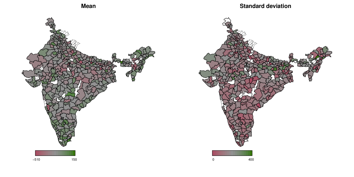
Figure 1: Spatial structure of stunting in India. The raw mean per district is given in the left figure, ranging from dark red (low stunting score), to dark green (higher scores). The right figure depicts the standard deviation of the stunting score in the district, ranging from dark red (no variation) to dark green (maximal variability). Dashed regions represent regions without data.

Table 1: Overview of india data.

		Min.	25% Qu.	Median	Mean	75% Qu.	Max.
Stunting	stunting	-599.00	-287.00	-176.00	-175.41	-65.00	564.00
BMI (child)	cbmi	10.03	14.23	15.36	15.52	16.60	25.95
Age (child; months)	cage	0.00	8.00	17.00	17.23	26.00	35.00
BMI (mother)	mbmi	13.14	17.85	19.36	19.81	21.21	39.81
Age (mother; years)	mage	13.00	21.00	24.00	24.41	27.00	49.00

4 The package gamboostLSS

The gamboostLSS algorithm is implemented in the publicly available R add-on package gamboostLSS (pkg:gamboostLSS:1.1-0). The package makes use of the fitting algorithms and some of the infrastructure of mboost (pkg:mboost:2.3-0). Furthermore, many naming conventions and features are implemented in analogy to mboost. By relying on the mboost package, gamboostLSS incorporates a wide range of base-learners and hence offers a great flexibility when it comes to the types of predictor effects on the parameters of a GAMLSS distribution. In addition to making the infrastructure available for GAMLSS, mboost constitutes a well-tested, mature software package in the back end. For the users of mboost, gamboostLSS offers the advantage of providing a drastically increased number of possible distributions to be fitted by boosting.

As a consequence of this partial dependency on mboost, we recommend users of gamboostLSS to make themselves familiar with the former before using the latter package. To make this tutorial self-contained, we try to shortly explain all relevant features here as well. However, a dedicated hands-on tutorial is available for an applied introduction to mboost (Hofner:mboost:2014).

4.1 Model-fitting

The models can be fitted using the function glmboostLSS() for linear models. For all kinds of structured additive models the function gamboostLSS() can be used. The function calls are as follows:

glmboostLSS(formula, data = list(), families = GaussianLSS(), control = boost_control(), weights = NULL, …) gamboostLSS(formula, data = list(), families = GaussianLSS(), control = boost_control(), weights = NULL, …)

The formula can consist of a single formula object, yielding the same candidate model for all distribution parameters. For example, R> glmboostLSS(y   x1 + x2 + x3 + x4, data = data) specifies linear models with predictors x1 to x4 for all GAMLSS parameters (here $\mu$ and $\sigma$ of the Gaussian distribution). As an alternative, one can also use a named list to specify different candidate models for different parameters, e.g. R> glmboostLSS(list(mu = y   x1 + x2, sigma = y   x3 + x4), data = data) fits a linear model with predictors x1 and x2 for the mu component and a linear model with predictors x3 and x4 for the sigma component. As for all R functions with a formula interface, one must specify the data set to be used (argument data). Additionally, weights can be specified for weighted regression. Instead of specifying the argument family as in mboost and other modeling packages, the user needs to specify the argument families, which basically consists of a list of sub-families, i.e., one family for each of the GAMLSS distribution parameters. These sub-families define the parameters of the GAMLSS distribution to be fitted. Details are given in the next section.

The initial number of boosting iterations as well as the step-lengths ($\nu_{\text{sl}}$; see Appendix LABEL:algorithm) are specified via the function boost_control() with the same arguments as in mboost. However, in order to give the user the possibility to choose different values for each additive predictor (corresponding to the different parameters of a GAMLSS), they can be specified via a vector or list. For example, one can specify:

R> boost_control(mstop = c(mu = 100, sigma = 200), R> nu = c(mu = 0.2, sigma = 0.01))

Specifying a single value for the stopping iteration mstop or the step-length nu results in equal values for all sub-families. The defaults is mstop = 100 for the initial number of boosting iterations and nu = 0.1 for the step-length. Additionally, the user can specify if status information should be printed by setting trace = TRUE in boost_control.

4.2 Distributions

Some GAMLSS distributions are directly implemented in the R add-on package gamboostLSS and can be specified via the families argument in the fitting function gamboostLSS() and glmboostLSS(). An overview of the implemented families is given in Table LABEL:tab:gamboostlss_families. The parametrization of the negative binomial distribution, the log-logistic distribution and the $t$ distribution in boosted GAMLSS models is given in mayretal. The derivation of boosted beta regression, another special case of GAMLSS, can for example be found in schmid2013beta. In our case study we will use the default GaussianLSS() family to model childhood malnutrition in India. The resulting object of the family looks as follows:

R> str(GaussianLSS(), 1) List of 2 $mu:Formalclass{}^{\prime }boost{}_{f}amily{}^{\prime }[package\mathrm{"}mboost\mathrm{"}]with10slots\text{Table 2Table 22Table 22Overviewofcode"families"thatareimplementedinpkggambo}$