Physical conditions of molecular gas in the Circinus galaxy
Multi-$J$ CO and C i³P${}_{1}\rightarrow^{3}$P₀ observations

We report mapping observations of the ¹²CO $J=3\rightarrow 2$, $4\rightarrow 3$, $6\rightarrow 5$, and $7\rightarrow 6$ transitions and the C i ³P${}_{1}\rightarrow^{3}$P₀ (C i) 492 GHz transition toward the central 40${}^{\prime\prime}\times$40^′′ region of the Circinus galaxy, using the Atacama Pathfinder EXperiment (APEX) telescope. We also detected ¹³CO $J=3\rightarrow 2$ at the central position of Circinus. These observations are to date the highest CO transitions reported in Circinus. With large velocity gradient (LVG) modeling and likelihood analysis we try to obtain density, temperature, and column density of the molecular gas in three regions: the nuclear region ($D<18^{\prime\prime}\sim$360 pc), the entire central 45^′′ ($D<45^{\prime\prime}\sim$ 900 pc) region, and the star-forming (S-F) ring (18${}^{\prime\prime}<D<45^{\prime\prime}$). In the nuclear region, we can fit the CO excitation with a single excitation component, yielding an average condition of $n_{\mathrm{H}_{2}}$$\sim$ $10^{3.2}$cm^-3 , $T_{\rm kin}$ $\sim$ 200  K, and ${\rm d}\varv/{\rm d}r$$\sim$ 3  km s^-1pc^-1. In the entire 45^′′ region, which covers both the nucleus and the S-F ring, two excitation components are needed with $n_{\mathrm{H}_{2}}$ $\sim$ 10^4.2 and 10^3.0 cm^-3 , $T_{\rm kin}$ $\sim$ 60 K and 30 K, and $M_{\rm H_{2}}$ $\sim$ $2.3\times 10^{7}$ M_⊙ and $6.6\times 10^{7}$ M_⊙, respectively. The gas excitation in the S-F ring can also be fitted with two LVG components, after subtracting the CO fluxes in the 18^′′ region. The S-F ring region contributes 80% of the molecular mass in the 45^′′ region. For the entire 45^′′ region, we find a standard conversion factor of $N({\rm H_{2}})/I_{\rm CO\ 1\rightarrow 0}$ = $0.37\times 10^{20}$ cm${}^{-2}({\rm K\ km\ s}^{-1})^{-1}$, about 1/5 of the Galactic disk value. The luminosity ratios of C i and ¹²CO $J=3\rightarrow 2$ ($R_{\rm CI/CO\ 3\rightarrow 2}$) in Circinus basically follow a linear trend, similar to that obtained in high-redshift galaxies. The average $R_{\rm CI/CO\ J=3\rightarrow 2}$ in Circinus is found to be $\sim$ 0.2, lying at an intermediate value between non-AGN nuclear region and high-redshift galaxies.

1 Introduction

Multiple rotational transitions of CO are a powerful tool to study the physical environment and the excitation conditions of molecular gas in galaxies. For galaxies harboring active galactic nuclei (AGN), the nuclear activity is often powered by the molecular gas surrounding the nuclear region, and the feedback – jets, winds, and radiation – may enhance or quench the star-forming (S-F) activity (e.g., Bundy et al., 2008; Sani et al., 2010). The excitation of molecular gas in the torus ($\sim$ a few pc to tens of pc) and in the circumnuclear disk (CND; a few tens to hundreds of pc) reflects the activity invoked by the illumination from the central supermassive black hole (SMBH) (e.g, Schinnerer et al., 2000; Pérez-Beaupuits et al., 2011; Harada et al., 2013). Because of its symmetry, molecular hydrogen (H₂) has no permanent dipole moment and its infrared transitions require high excitation conditions, thus the H₂ emission is not able to trace molecular clouds (e.g., Kennicutt & Evans, 2012). Carbon monoxide (CO), the second most abundant molecule, has a dipole moment of 0.112 Debye and is heavy enough for a rotational spectrum accessible at submillimeter (submm) wavelengths, tracing both cold and warm gas. CO lines are therefore regarded as the best tracers to the probe the physical properties and the excitation conditions of the entire molecular gas reservoir (e.g., Mao et al., 2000; van der Werf et al., 2010; Papadopoulos et al., 2012b).

So far, in nearby galaxies most studies of the molecular gas emission focus on the $J$=1$\rightarrow$0, 2$\rightarrow$1, and 3$\rightarrow$2 transitions of CO (e.g., Braine et al., 1993; Dumke et al., 2001; Israel & Baas, 2003; Wilson et al., 2011). At high redshifts mid-$J$ (4$\leq$$J$$\leq$8) CO transitions are almost exclusively measured (e.g., Omont et al., 1996; Carilli et al., 2010; Wang et al., 2010). Therefore, observations of the mid-$J$ transitions in some nearby galaxies are essential to investigate the gas excitation, as reference of the high-redshift galaxies. Such studies have been focused on nearby S-F galaxies such as NGC 253, IC 342, and NGC 4038, (e.g., Güsten et al., 2006; Hailey-Dunsheath et al., 2008; Bayet et al., 2009), but only a few nearby galaxies with prominent AGNs have been studied so far in these mid-$J$ CO lines (e.g, NGC 1068; Israel, 2009a; Spinoglio et al., 2012).

The Circinus galaxy is a prototypical Seyfert-2 galaxy located in the southern sky, at a small distance of $D\sim$ 4 Mpc (e.g., Maiolino et al., 1998; Tully et al., 2009). Although it has a large angular size ($\geq$ 80^′) at optical wavelengths and in atomic gas (Hi), Circinus was not discovered until the 1970s (Freeman et al., 1977; Jones et al., 1999), because it is located only $\sim$ 4$\degr$ above the Galactic plane with a Galactic visual extinction of 4.8 mag (e.g., Schlegel et al., 1998). H₂O mega-masers at both mm and submm wavelengths were found in the center of Circinus (e.g., Greenhill et al., 2003; Hagiwara et al., 2013), indicating a molecular torus around the central SMBH. The mass of the SMBH is estimated to be $1.7\pm 0.3\times 10^{6}$ M_⊙  (e.g., Greenhill et al., 2003), and the torus accretion rate is as high as $\sim$ 20% of the Eddington luminosity (e.g., Tristram et al., 2007).

A large amount of molecular gas in Circinus was detected through the ¹²CO $J=1\rightarrow 0$ and ¹³CO $J=1\rightarrow 0$ observations by Aalto et al. (1991), with the Swedish-ESO 15m Submillimeter Telescope (SEST). Besides the isotopologues of CO lines (i.e., ¹³CO, C¹⁸O), Curran et al. (2001) contained rich molecular spectra, including lines from HCN, HNC, and HCO⁺, which indicate the presence of highly excited dense gas in the central region of Circinus. Furthermore, Circinus was also mapped in the $J=1\rightarrow 0$, $2\rightarrow 1$, and $3\rightarrow 2$ transitions of CO (Curran et al., 2001, 2008). With the deconvolved ¹²CO $J=2\rightarrow 1$ map, Johansson et al. (1991) found a face-on molecular ring structure, which seems to be associated with the S-F ring shown in H$\alpha$ (Marconi et al., 1994). Curran et al. (1998, 1999) found that the gas kinematics could be modeled with a highly inclined molecular ring and two outflows using the ¹²CO $J=2\rightarrow 1$ data.

Hitschfeld et al. (2008) observed the ¹²CO $J=4\rightarrow 3$ and C i ³P${}_{1}\rightarrow^{3}$P₀ (hereafter C i 1$\rightarrow$0) lines in the center of Circinus with the NANTEN-2 4 m telescope. They studied the molecular gas excitation and predicted that the global CO cooling curve peaks at the $J=4\rightarrow 3$ transition, however, higher-$J$ CO transitions are still needed to test their model and to compare the results with other nearby galaxies at similar scales. The turnover of the global CO line ladders is also very important for comparisons with molecular line surveys of gas-rich S-F objects (e.g., Blain et al., 2000; Combes et al., 1999; Geach & Papadopoulos, 2012; Carilli & Walter, 2013). With the large beam sizes of the single dish telescopes in the published low-$J$ observations, it is in any case difficult to explore the excitation conditions in the very central region of Circinus. For these reasons, we have performed high-resolution mapping observations of mid-$J$ CO lines and the C i $1\rightarrow 0$ transition in the central region of Circinus.

This article is organized as follows. Sect. 2 describes the observational methods and data reduction procedure. Sect. 3 presents the spectra and maps. In Sect. 4, the CO lines are analyzed using large velocity gradient (LVG) modeling. The discussion of the data and our modeling results are also presented. In Sect. 5, our findings and conclusions are summarized. Throughout this paper, we adopt for the distance of Circinus a value of 4.2 Mpc (Freeman et al., 1977). Thus 1^′′ corresponds to $\sim$20 pc.

2 Observations & data reduction

2.1 CO and C i 1$\rightarrow$0 spectral line observations

Table 1: Parameters of ¹³CO, ¹²CO, and C iobservations

Transitions	Date	Receiver	$\eta_{\rm mb}$	$\eta_{\rm f}$	Jy/K	$pwv$	$T_{\rm sys}$	Map Size	Obs. Modea
						(mm)	(K)	(R.A.$\times$ Dec.)
13CO $J=3\rightarrow 2$	2006-Jul-23	APEX2A	0.73	0.97	40	1.1	190 $\cdots$ 210	central pointb	ON-OFF
	2009-Oct-16	APEX2A	0.73	0.97	40	1.3	500 $\cdots$ 700	central point	ON-OFF
12CO $J=3\rightarrow 2$	2006-Jun-27	APEX2A	0.73	0.97	41	1.1	150 $\cdots$ 160	central point	ON-OFF
	2006-Jul-23	APEX2A	0.73	0.97	41	1.1	180 $\cdots$ 220	$40\hbox{${}^{\prime\prime}$}\times 40\hbox{${}^{\prime\prime}$}$	RASTER
	2007-Jun-30	APEX2A	0.73	0.97	41	1.1	230 $\cdots$ 250	$40\hbox{${}^{\prime\prime}$}\times 25\hbox{${}^{\prime\prime}$}$	RASTER
	2008-Dec-26	APEX2A	0.73	0.97	41	1.1	300 $\cdots$ 345	central point	ON-OFF
	2009-Oct-16	APEX2A	0.73	0.97	41	1.1	440 $\cdots$ 450	central point	ON-OFF
	2010-Jul-14	FLASH345	0.73	0.97	41	0.6	190 $\cdots$ 210	$20\hbox{${}^{\prime\prime}$}\times 30\hbox{${}^{\prime\prime}$}$	RASTER
	2010-Nov-15	FLASH345	0.73	0.97	41	1.5	350 $\cdots$ 380	central point	ON-OFF
12CO $J=4\rightarrow 3$	2009-Jun-07	FLASH460	0.60	0.95	48	0.60	500 $\cdots$ 600	$30\hbox{${}^{\prime\prime}$}\times 40\hbox{${}^{\prime\prime}$}$	RASTER
12CO $J=6\rightarrow 5$	2009-Jun-13	CHAMP+-I	0.52	0.95	53	0.52	1500 $\cdots$ 2100	$80\hbox{${}^{\prime\prime}$}\times 60\hbox{${}^{\prime\prime}$}$	OTF
	2009-Aug-10	CHAMP+-I	0.52	0.95	53	0.27	1000 $\cdots$ 1300	$80\hbox{${}^{\prime\prime}$}\times 60\hbox{${}^{\prime\prime}$}$	OTF
12CO $J=7\rightarrow 6$	2009-Jun-13	CHAMP+-II	0.49	0.95	70	0.49	4000 $\cdots$ 9000	$80\hbox{${}^{\prime\prime}$}\times 60\hbox{${}^{\prime\prime}$}$	OTF
	2009-Aug-10	CHAMP+-II	0.49	0.95	70	0.49	2500 $\cdots$ 4000	$80\hbox{${}^{\prime\prime}$}\times 60\hbox{${}^{\prime\prime}$}$	OTF
C i 1$\rightarrow$0	2010-Jul-14	FLASH460	0.60	0.95	50	0.60	700 $\cdots$ 1000	$15\hbox{${}^{\prime\prime}$}\times 25\hbox{${}^{\prime\prime}$}$	ON-OFF

a) ON-OFF: position switching; RASTER: raster scan; OTF: On-The-Fly scan.
b) We adopt $\alpha(J2000)=14^{h}13^{m}10.0^{s}$, $\delta(J2000)=-65^{\circ}20{\hbox{${}^{\prime}$}}21.\!\!{\hbox{${}^{\prime\prime}$}}$0 as the central position of Circinus.

The observations were performed with the 12-m Atacama Pathfinder EXperiment (APEX) telescope on the Chajnantor Plateau in Chile. Most observations were obtained in good ($\tau<$ 0.3 at 810 GHz) to median ($\tau\sim$ 0.6 – 1 at 345 GHz and 460 GHz) weather conditions during several runs between 2006 and 2010. The C i $1\rightarrow 0$ data and a part of the ¹²CO $J=3\rightarrow 2$ data were taken simultaneously on 14 July, 2010, with the FLASH dual-frequency receiver. ¹²CO $J=6\rightarrow 5$ and $7\rightarrow 6$ maps were obtained simultaneously with the CHAMP⁺ 7-pixel receiver array (Kasemann et al., 2006), during June and August 2009. Single point ¹³CO $J=3\rightarrow 2$ measurements were taken toward the central position of Circinus ($\alpha(J2000)=14^{h}13^{m}10.0^{s}$, $\delta(J2000)=-65^{\circ}20{\hbox{${}^{\prime}$}}21.\!\!{\hbox{${}^{\prime\prime}$}}$0) in July 2006 and October 2009. Fast Fourier Transform Spectrometer (FFTS) backends (Klein et al., 2006) were employed in all observations, with channel spacings of 1 or 2 MHz, which were then smoothed to suitable velocity resolutions in the data reduction.

We determined focus every four to five hours on Saturn and Jupiter. We calibrated pointing every one to two hours. This ensures 2^′′ (rms) pointing uncertainties derived from G327.3–0.6 for ¹²CO $J=6\rightarrow 5$ and ¹²CO $J=7\rightarrow 6$. The angular resolution varies from 18^′′ (for ¹²CO $J=3\rightarrow 2$) to 8^′′(for ¹²CO $J=7\rightarrow 6$), according to the observing frequencies. At the 345 GHz and 460 GHz bands, because there was no suitable strong nearby pointing calibrator at similar elevations, we made pointing calibrations with planets, NGC6334I (about 40$\degr$ away from Circinus), and the strong ¹²CO $J=3\rightarrow 2$ emission from Circinus itself. Here we estimate systematic position errors to be $\sim$5^′′ (rms).

We carried out the mapping observations in raster scan or on-the-fly (OTF) mode. We used a position of 10^′ to the east of the center of Circinus as the sky reference. Except for ¹³CO $J=3\rightarrow 2$, which was only measured at the central position of Circinus, all CO lines are fully sampled in the innermost $\sim 40\hbox{${}^{\prime\prime}$}\times 40\hbox{${}^{\prime\prime}$}$ ($\sim 800\times 800$ pc) with Nyquist sampling. The mapped sizes of ¹²CO $J=6\rightarrow 5$ and $7\rightarrow 6$ are about 80${}^{\prime\prime}\times$60^′′, but the inner $40^{\prime\prime}\times 40^{\prime\prime}$ region has a better rms noise level than that in the outer region because the integration time was longer in the center. C i $1\rightarrow 0$ is mapped in a region of size $\sim 15\hbox{${}^{\prime\prime}$}\times 25\hbox{${}^{\prime\prime}$}$.

All observations were performed with frequencies corresponding to a velocity of $\varv_{\rm LSR}$$\sim$420  km s^-1 (Local Standard of Rest). We list the observation date, instruments, typical rms. noise levels, system temperatures, telescope efficiencies, and map sizes for different epochs in Tables 1 and 2.

2.2 Spectral line data reduction

All spectral line data are reduced with the CLASS/GILDAS package. We inspect each spectrum by eye and classify the spectral quality from baseline flatness and system temperature levels. About 5% of the spectra are discarded, except for ¹³CO $J=3\rightarrow 2$ and ¹²CO $J=7\rightarrow 6$, for which 50% and 20% of the data have to be dropped respectively, because of unstable baselines. Linear baseline is subtracted for each individual spectrum. All spectra are then coadded and resampled to $5$ km s^-1 velocity resolution.

We find that the emission peaks and the intensity distributions of ¹²CO $J=3\rightarrow 2$, $4\rightarrow 3$, and C i 1$\rightarrow$0 observed during different epochs have offsets of $\sim 3-5^{\prime\prime}$, which are likely caused by our limited pointing accuracy. These offsets are systematic for each observing epoch. Within the limits of pointing errors ($<1/4$ of the beam size), relative intensity distributions are the same for the observed maps. We assume that the central position of Circinus should show particularly strong CO emission with a symmetrical line profile, and this profile should also correspond to the peak position of the integrated intensity in an individual map. We fit the map distributions and shift the positions of ¹²CO $J=3\rightarrow 2$, $4\rightarrow 3$, and C i 1$\rightarrow$0 accordingly, and then coadd the maps to improve signal-to-noise ratios. From several measurement epochs, we estimate calibration uncertainties to be 10% for ¹²CO $J=3\rightarrow 2$ and $4\rightarrow 3$, and 15% for ¹²CO $J=6\rightarrow 5$ and $7\rightarrow 6$.

We convert the antenna temperature ($T_{\rm A}^{\star}$) to the main beam brightness temperature ($T_{\rm mb}$) scale, using ${T_{\rm mb}=T_{\rm A}^{\star}\cdot\eta_{\rm f}/\eta_{\rm mb}}$, where $\eta_{\rm f}$ and $\eta_{\rm mb}$ are the forward hemisphere and main beam efficiencies of the telescope. We list them in Table 1. All spectra presented in this paper are in units of $T_{\rm mb}$(K). In Table 2 we list frequencies, angular resolutions, and noise levels of the reduced data.

For each transition, we combine all the calibrated spectra and use the gridding routine XY_MAP in CLASS to construct datacubes, with weightings proportional to 1/$\sigma^{2}$, where $\sigma$ is the rms. noise level. This routine convolves the gridded data with a Gaussian kernel of full width to half maximum (FWHM) $\sim$1/3 the telescope beam size, yielding a final angular resolution slightly coarser than the original beam size. For the analysis below, we further convolve the datacubes to several angular resolutions to facilitate comparisons with data from the literature.

Table 2: Parameters of the observed lines

Transitions	$\nu_{rest}$	Resolution	rmsa
	(GHz)	(′′)	(K)
13CO $J=3\rightarrow 2$	330.588	19.0	0.02
12CO $J=3\rightarrow 2$	345.796	18.2	0.06
12CO $J=4\rightarrow 3$	461.041	14.0	0.1
12CO $J=6\rightarrow 5$	691.473	9.4	0.3
12CO $J=7\rightarrow 6$	806.652	8.2	1.0
C i 1$\rightarrow$0	492.161	13.5	0.12

a) 1$\sigma$ noise level in units of $T_{\rm mb}$ calculated from the datacubes with a channel width of 5 km s^-1 .

2.3 Other archival data

We obtained a 70 $\mu$m image observed with the Photoconductor Array Camera and Spectrometer (PACS) on board the Herschel space telescope through the Herschel Science Archive. We downloaded the post processed data of level 2.5. The observation ID is 1342203269, and it contains data observed on 20 August 2010. We also used an archival H$\alpha$ image of the Hubble Space Telescope (HST) (Wilson et al., 2000), downloaded from the NASA/IPAC Extragalactic Database (NED).

3 Results

3.1 Spatial distributions

3.1.1 Herschel 70 $\mu$m and HST maps of the Circinus galaxy

The left panel of Fig. 1 shows Herschel 70 $\mu$m contours overlaid on an HST H$\alpha$ image (Wilson et al., 2000). The 70 $\mu$m emission has a concentration in the very central region, and an extended emission out to about 40^′′ (in diameter). The H$\alpha$ emission shows structures of both the S-F ring and the central nuclear region. Therefore, we separate the center of Circinus into three regions: the nuclear region ($D<18^{\prime\prime}\sim$360 pc), the entire central 45^′′ ($D<45^{\prime\prime}\sim$ 900 pc) region, and the S-F ring region (18${}^{\prime\prime}<D<45^{\prime\prime}$). We define the H$\alpha$ bright ring like structure as the S-F ring, rather than the ring structure modeled in Curran et al. (1999). The concentric circles show the nuclear region (white) and the entire central region (red) including both the nucleus and the S-F ring. The peak of the 70 $\mu$m emission is consistent with the center of the CO emission (e.g., Curran et al., 2001), and has a slight shift down to the south of the H$\alpha$ peak, which is likely attenuated by the dust extinction. The central 18^′′ region contributes $\sim$ 20% of the 70 $\mu$m emission of the entire galaxy. These features are also consistent with the Spitzer mid-infrared images (For et al., 2012).

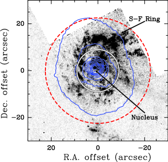
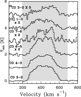
Figure 1: The left panel shows the Herschel 70 $\mu$m contours overlaid on an H$\alpha$ image of the HST (Wilson et al., 2000). The contour levels are 500, 1000, 2000, 3000, and 4000 MJy/sr. The concentric circles show the beam sizes of ¹²CO $J=3\rightarrow 2$ for APEX (18^′′, white thick line) and ¹²CO $J=1\rightarrow 0$ for SEST (45^′′, red dashed line). The right panel shows the CO spectra observed in the central position. ¹²CO $J=6\rightarrow 5$, $7\rightarrow 6$, and C i are multiplied by a factor of 2, and ¹³CO $J=3\rightarrow 2$ is multiplied by a factor of 5. The (shaded) line emission ranges from $\sim$200 to $\sim$700 km s^-1 .

3.1.2 CO & C i 1$\rightarrow$0 spectra

The CO and C i  spectra from the central position (Fig. 1, right panel) are shown with their original angular resolutions (before the convolution in XY_MAP). Although the ¹²CO $J=7\rightarrow 6$ and C i lines have relatively low S/N, all of the line profiles look fairly similar, i.e., their intensity ratios are constant to within ∼30% as a function of velocity. This implies that overall, the gas components probed by the different lines follow the same kinematics.

We convolve Gaussian kernels with all datacubes to match the angular resolutions of the low-$J$ CO data. Using the beam matched datacubes, we extract spectra in the central position and calculate the integrated line intensities in the velocity range from 200 km s^-1 to 700 km s^-1 . Table  3 summarizes the observed line properties at the angular resolutions of 18^′′ and 45^′′.

Fig. 2 shows spectra of C i and ¹²CO $J=3\rightarrow 2$ from the central region of Circinus. We obtained these two lines simultaneously, free from pointing inaccuracy. We overlay their spectra in their original angular resolutions, $\sim$12.5^′′ for C i and $\sim$18^′′ for ¹²CO $J=3\rightarrow 2$. At most positions, there is no obvious discrepancy between the line profiles of ¹²CO $J=3\rightarrow 2$ and C i, neither in the central position nor at the edges of the mapped region.

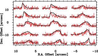
Figure 2: C i 1$\rightarrow$0 and ¹²CO $J=3\rightarrow 2$ spectra from the central region of the Circinus galaxy. The C i spectra are relatively noisier and are presented in red, while the ¹²CO $J=3\rightarrow 2$ profiles are plotted in black. To reach similar intensities, C i is scaled up by a factor of three.

Table 3: CO line intensities

Transitions	Beam=18′′			Beam=45′′
	$W{{}_{\rm line}}$a	$F{{}_{\rm line}}$	$L^{\prime}{{}_{\rm line}}/L^{\prime}_{\rm CO3-2}$	$W{{}_{\rm line}}$	$F{{}_{\rm line}}$	$L^{\prime}{{}_{\rm line}}/L^{\prime}{\rm{}_{CO3-2}}$
	K km s-1	Jy km s-1	–	K km s-1	Jy km s-1	–
12CO $J=1\rightarrow 0$	–	–	–	180$\pm$35b	3.51$\times 10^{3}$	1
12CO $J=2\rightarrow 1$	–	–	–	144$\pm$25b	1.42$\times 10^{4}$	0.83$\pm$0.20
12CO $J=3\rightarrow 2$	310$\pm$20	0.97$\times 10^{4}$	1	140$\pm$20	2.49$\times 10^{4}$	0.79$\pm$0.16
12CO $J=4\rightarrow 3$	240$\pm$20	1.17$\times 10^{4}$	0.77$\pm$ 0.2	80$\pm$15	2.51$\times 10^{4}$	0.44$\pm$0.09
12CO $J=6\rightarrow 5$	140$\pm$15	1.44$\times 10^{4}$	0.45$\pm$ 0.08	35$\pm$5	2.48$\times 10^{4}$	0.19$\pm$0.03
12CO $J=7\rightarrow 6$	55$\pm$7	0.97$\times 10^{4}$	0.18$\pm$ 0.03	19$\pm$5	1.73$\times 10^{4}$	0.11$\pm$0.03
13CO $J=1\rightarrow 0$	–	–	–	13$\pm$2.5	230	0.07$\pm$0.02
13CO $J=2\rightarrow 1$	–	–	–	12.5$\pm$2.5	1300	0.07$\pm$0.02
13CO $J=3\rightarrow 2$	24 $\pm$ 5	740	0.07$\pm$0.02	9.5$\pm$3.0c	1850	0.05$\pm$0.02
C i 1$\rightarrow$0	100 $\pm$ 25	5$\times 10^{3}$		45 $\pm$ 10	1.4$\times 10^{4}$

3.1.3 CO and C i  maps

Fig. 3 presents the integrated intensity images (moment-zero maps) of all ¹²CO transitions mapped with the APEX telescope. The dotted thick (red) contour lines present half of the peak intensity level for each map. The CO emission of all transitions is well confined within the central 40${}^{\prime\prime}\times 40^{\prime\prime}$ region. To increase the S/N level of ¹²CO $J=7\rightarrow 6$, we convolved it to the angular resolution of the ¹²CO $J=3\rightarrow 2$ map. The ¹²CO $J=6\rightarrow 5$ and $J=7\rightarrow 6$ distributions show elongations along the major axis, i.e., along the direction from the northeast to the southwest. The thin dotted contours (blue) in the ¹²CO $J=6\rightarrow 5$ and $J=7\rightarrow 6$ maps mark the regions with almost uniform scanning coverage in the OTF mappings, so these regions have lower noise levels than those outside. We mask the corners of the ¹²CO $J=7\rightarrow 6$ image to avoid displaying regions farther out with high noise and poor baselines.

To explore the sizes of the emitting regions in different CO transitions, we deconvolve the moment-zero maps with circular Gaussian beams, and fit the source sizes using two-dimensional Gaussian models. For ¹²CO $J=3\rightarrow 2$, $4\rightarrow 3$, and $6\rightarrow 5$, the beam sizes (FWHM) of 18^′′, 14.0^′′, and 9.4^′′ (see Table 2) are adopted to deconvolve the images, respectively. The S/N ratio of the ¹²CO $J=7\rightarrow 6$ map is not high enough to provide reliable fitting results. We list the fitting parameters in Table 4. For ¹²CO $J=3\rightarrow 2$ we get a position angle of 33.5$\degr$, which is adopted in the following analysis to define the major axis of molecular gas emission. This result is also close to the position angle of 34^∘ derived from ¹²CO $J=1\rightarrow 0$ and $2\rightarrow 1$ maps (Curran et al., 2008). The fitted position angle of C i 1$\rightarrow$0 is 65.5$\degr$, which is much larger than those determined from the CO images. This is most likely a consequence of the small size of our C i map. Because C i emission follows CO in all studied cases (e.g., Ikeda et al., 2002; Zhang et al., 2007), a different distribution is highly unlikely.

Table 4: Fitting parameters of CO moment-zero maps.

	Apparent Size		Deconvolved Size
Line	Major Axis	Minor Axis	Major Axis	Minor Axis	Pos. Angle
	(′′)	(′′)	(′′)	(′′)	($\degr$)
12CO $J=3\rightarrow 2$	28.1$\pm$0.4	27.1$\pm$ 0.4	20.6 $\pm$0.4	19.1$\pm$0.4	33.5
12CO $J=4\rightarrow 3$	24.0$\pm$0.5	21.4$\pm$ 0.5	19.2$\pm$0.5	15.8$\pm$0.4	36.0
12CO $J=6\rightarrow 5$	17.6$\pm$0.5	14.2$\pm$ 0.5	14.8$\pm$0.6	10.5$\pm$0.5	40.0
C i 1$\rightarrow$0a	21.4$\pm$3.2	14.4$\pm$ 0.9	16.7$\pm$3	5.2$\pm$1	65.5

a) The fitted size of the minor axis and the position angle could be affected by incomplete mapping. Curran et al. (2008) obtain 34^∘$\pm$4^∘ as the large scale position angle from CO $J$=1$\rightarrow$0 and 2$\rightarrow$1 data.

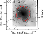
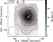
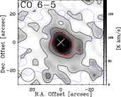
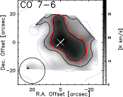
Figure 3: Moment-zero images of multiple-$J$ CO transitions. Big crosses mark the central position of Circinus; small crosses in the upper panels denote the sampled positions. Upper left: ¹²CO $J=3\rightarrow 2$; upper right: ¹²CO $J=4\rightarrow 3$; lower left: ¹²CO $J=6\rightarrow 5$; lower right: ¹²CO $J$ = 7 $\rightarrow$ 6. Circles in the lower left of each panel show the beam. The ¹²CO $J=7\rightarrow 6$ map was convolved to an angular resolution of 18^′′. Contour levels are 20, 60, …, 180 K km s^-1 in steps of 40 K km s^-1  for ¹²CO $J=3\rightarrow 2$, $J=4\rightarrow 3$, and $J=6\rightarrow 5$, and 10, 20, 30 K km s^-1  for ¹²CO $J=7\rightarrow 6$ (1 $\sigma=$ 1.9, 3, 10, and 3 K km s^-1  for ¹²CO $J=3\rightarrow 2$, $J=4\rightarrow 3$, $J=6\rightarrow 5$, and $J=7\rightarrow 6$). Red (thick dotted) contours present the half maximum level of all images. The thin dotted lines in the lower two panels denote the regions that have been scanned with higher S/N than other regions farther away from the centers (see Sects.  2 and 3.1.3). The outer dotted lines in the ¹²CO $J=7\rightarrow 6$ map are related to masking.

In Fig. 4, we present the integrated intensity image of C i 492 GHz emission. In spite of a smaller mapping area compared to CO, the thick dotted (red) line denoting the half maximum level of the emission peak is still mostly within the confines of the map. The detected structure covers an angular distance of $\sim$20^′′ from northeast to southwest, corresponding to 400 pc on the linear scale. Both the nuclear region and the S-F ring seen in the ¹²CO $J=1\rightarrow 0$ and $2\rightarrow 1$ images (Curran et al., 1998) are covered by the C i 1$\rightarrow$0 map.

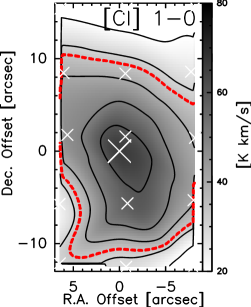
Figure 4: The 492 GHz C i $1\rightarrow 0$ integrated intensity image of the central part of the Circinus galaxy. Plotted contour levels are: 20 (6 $\sigma$), 30, 40, 50, and 60 mK km s^-1 . The red contour presents the half maximum level of the C i emission. The beam size (FWHM) is 13.5^′′.

3.2 Gas kinematics

3.2.1 CO channel maps

In Fig. 5, we plot the channel maps of ¹²CO $J=3\rightarrow 2$, $4\rightarrow 3$, and $6\rightarrow 5$. The northeastern side of Circinus is approaching and the southwestern side is receding. ¹²CO $J=6\rightarrow 5$ is highly concentrated near the peaks of the ¹²CO $J=3\rightarrow 2$ and $4\rightarrow 3$, i.e., near the central position of Circinus. The systematic velocity variations of different CO transitions are apparent. The emission of all three lines is particularly strong at the velocity bins of 300–400 km s^-1 and 450–550 km s^-1 , and the brightness temperature peaks even exceed those in the central velocity bin ranging from 400 to 450 km s^-1 . The ¹²CO $J=4\rightarrow 3$ and $6\rightarrow 5$ emission drops faster than that of ¹²CO $J=3\rightarrow 2$ when the velocity is higher than 550 km s^-1 and lower than 300 km s^-1 .

3.2.2 CO P-V diagrams

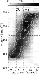
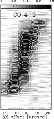
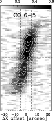
Figure 6: Position-velocity (P-V) maps of CO emission from the Circinus galaxy. From left to right: P-V diagrams of ¹²CO $J=3\rightarrow 2$, ¹²CO $J=4\rightarrow 3$, and ¹²CO $J=6\rightarrow 5$. The slice is taken along the major axis obtained from ¹²CO $J=3\rightarrow 2$ (position angle: 33.$\!\!{}^{\circ}$5, see Table 4) and the direction is from northeast (bottom) to southwest (top). The contours are from 30% to 90% of the peak intensities with a spacing of 20%.

Fig. 6 shows the position-velocity (P-V) diagrams of ¹²CO $J=3\rightarrow 2$, $4\rightarrow 3$, and $6\rightarrow 5$, along the major axis of Circinus. We make cuts with a position angle of 33.5$\degr$, which is from the fitting result of Sect. 3.1.3 (see also Table 4). In the P-V diagram of ¹²CO $J=3\rightarrow 2$, the ridge of maximum intensity covers a velocity range of about 400 km s^-1 , in accordance with the high inclination ($i$$\sim$65–78^∘; Curran et al., 2008) of the galaxy, over a region of roughly $\pm$10^′′. The rotation field in this area is characterized by a velocity gradient of $d\varv/d\theta=400$ km s^-1 /20^′′ ($\sim$20 km s^-1 /arcsec), corresponding to $d\varv/dr\sim$ 1.0 km s^-1pc^-1in the plane of the galaxy, when an inclination angle of 65$\degr$ is adopted (Freeman et al., 1977). The higher-$J$ level and the higher the angular resolution, the steeper the rotation curve appears. The ¹²CO $J=4\rightarrow 3$ distribution looks similar to that of ¹²CO $J=3\rightarrow 2$, but appears to be slimmer because of the higher angular resolution. For ¹²CO $J=6\rightarrow 5$, the ridge of maximum intensity covers a velocity range of $\sim$350 km s^-1 in a small region encompassing offsets of $\pm$5^′′. We derive a velocity gradient of $\sim 350$ km s^-1 /10^′′ (${\rm d}\varv/{\rm d}r$$\sim 1.5$ km s^-1pc^-1), which corresponds to ${\rm d}\varv/{\rm d}r$ $\sim$1.7 km s^-1pc^-1 when an inclination angle of $65\degr$ is applied. Limited by the spatial resolution, these velocity gradients only provide lower limits for the actual rotational motions in the central region of Circinus.

We estimate the dynamical mass from $M_{\rm dyn}$[M_⊙] = 230 $\times$ $\varv^{2}_{\rm rot}$[km s^-1 ] $\times$ $r[{\rm pc}]$ (e.g., Schinnerer et al., 2000), where $\varv_{\rm rot}$ is the inclination-corrected rotation speed in km s^-1 , and $r$ is the radius in pc. We find a rotation velocity $\varv_{\rm rot}$ = (340 km s^-1/2)/sin(65$\degr\pm 5\degr$) $\sim 190\pm 10$ km s^-1 , and derive dynamic masses of $M_{\rm dyn}$ = 1.4$\pm$0.1 $\times$ 10⁹ M_⊙ within 180 pc of the center, and 3.6$\pm$0.4 $\times$10⁹ M_⊙ within a galactocentric radius of 450 pc. The latter is consistent with the dynamical mass of 3.3$\pm$0.3 $\times$ 10⁹ M_⊙ estimated for an outer radius of 560 pc by Curran et al. (1998).

Unlike the case of the moment-zero maps, where all CO emission peaks at the central position, the CO transitions in the P-V diagrams mainly peak at the edges of the velocity distributions on the major axis. This scenario indicates a central molecular void and a circumnuclear ring. The P-V diagram of ¹²CO $J=3\rightarrow 2$ is, within the errors, symmetric for the lowest emission levels around the AGN, with respect to a radial velocity of 430 $\pm$20 km s^-1 . The earlier adopted central positions (Figs. 2–6) are consistent with the dynamical center of the galaxy and the velocity can be interpreted as the systemic velocity ($\varv_{\rm sys}$).

4 Excitation conditions and discussions

Including our new measurements, ¹²CO has been observed toward the nuclear region of Circinus in all transitions up to $J=7\rightarrow 6$, except for $J=5\rightarrow 4$ (e.g., Aalto et al., 1991; Israel, 1992; Elmouttie et al., 1997; Curran et al., 1998, 2001; Hitschfeld et al., 2008). The rare isotopologue ¹³CO has been measured in transitions from $J=1\rightarrow 0$ to $J=2\rightarrow 1$ (e.g., Curran et al., 1998, 2001; Hitschfeld et al., 2008), and $J=3\rightarrow 2$ (this paper). The low-$J$ transitions were observed mostly with SEST 15 m and Mopra 22 m (equivalent 15 m beam size at 115 GHz; Elmouttie et al., 1997), while the mid-$J$ transitions were observed with the APEX 12 m and the NANTEN-2 4 m telescopes. Table 3 summarizes ¹²CO and ¹³CO observations collected from the literature.

The wide range of critical density (from $\sim 3\ \times 10^{2}$cm^-3  for CO $J$ = 1$\rightarrow$0 to $\sim 4\ \times 10^{5}$ cm^-3  for CO $J$=7$\rightarrow$6) and $E_{\rm upper}/k_{\rm B}$ (from 5.5 K to 155 K) of CO lines from $J=1\rightarrow 0$ up to $J=7\rightarrow 6$ allows us to probe the molecular gas physical conditions ranging from the cold and low-density average states in giant molecular clouds all the way up to the state of the gas found only near their S-F regions (e.g., Yang et al., 2010; Bradford et al., 2005). Bright ¹²CO $J=6\rightarrow 5$ and $J=7\rightarrow 6$ emission in Circinus implies that there is a large amount of molecular gas in a highly excited phase, while the low-$J$ CO transition lines are also sensitive to the colder and possibly more diffuse gas phase.

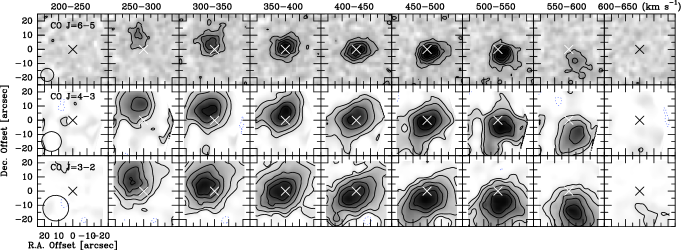
Figure 5: CO channel maps of the central region of the Circinus galaxy. The velocity range is given at the top, and the nuclear position of the Circinus galaxy is labeled by white crosses. Beam sizes are shown in the panels at the left hand side. Upper panels: ¹²CO $J=6\rightarrow 5$ channel maps. The contours are from 0.1 ($2\sigma$) to 0.5 K with a spacing of 0.1 K. Middle panels: ¹²CO $J=4\rightarrow 3$ channel maps. The contours are –0.1 (dotted) and 0.1 to 1.0 K km s^-1 , the latter with a spacing of 0.1 K. The 3 $\sigma$ noise level corresponds to 0.1 K. Lower panels: ¹²CO $J=3\rightarrow 2$ channel maps. The contours are the same as for ¹²CO $J=4\rightarrow 3$. The 5 $\sigma$ noise level corresponds to 0.1 K.

4.1 The large velocity gradient radiative transfer model

To estimate the physical parameters of the molecular gas, we employ a large velocity gradient (LVG) radiative transfer model (e.g., Scoville & Solomon, 1974; Goldreich & Kwan, 1974) to constrain the excitation conditions. We adopt an escape probability of $\beta=(1-e^{-\tau})/\tau$, which implies a spherical geometry and an isothermal environment. While multiple phases of physical conditions should exist in the molecular cloud complexes of Circinus, it is difficult to disentangle them (but see below). We thus adopt homogeneous clouds in the LVG modeling to constrain the average physical properties of molecular gas.

We proceed with a three-dimensional parameter grid with regularly spaced kinetic temperature ($T_{\rm kin}$), H₂ number density ($n_{\mathrm{H}_{2}}$), and fractional abundance versus velocity gradient ($x_{\rm CO}/({\rm d}\varv/{\rm d}r)$) as input, where $x_{\rm CO}$ is the abundance ratio of CO relative to H₂. In the following analysis, $x_{{}^{12}{\rm CO}}$ is fixed to 8$\times 10^{-5}$ (Frerking et al., 1982). The input parameter grid consists of $T_{\rm kin}$ from $10^{1}$ to 10³ K, $n_{\mathrm{H}_{2}}$ from 10² to 10⁷cm^-3 , and ${\rm d}\varv/{\rm d}r$ from 10⁰ to 10³ km s^-1pc^-1. We sample all these parameters with logarithmic steps of 0.1. We adopt RADEX (van der Tak et al., 2007) to generate the model grids. We excluded all solutions with $\tau>100$ and the solutions did not reach convergence.

We adopt the ¹²CO to ¹³CO abundance ratio ($R_{1213}$) to be 40 in the following analysis. It is intermediate between the values measured near the Galactic center and the solar circle (e.g., Wilson & Matteucci, 1992). This value is also consistent with the ratios derived in the active nuclear regions of nearby galaxies (e.g., NGC 1068, NGC 253, NGC 4945; Henkel & Mauersberger, 1993; Langer & Penzias, 1993; Wilson & Rood, 1994; Henkel et al., 2014). We do not adopt $R_{1213}$=60-80 given in Curran et al. (2001), because we obtained 25% higher ¹²CO $J=3\rightarrow 2$ flux (confirmed with several redundant observations) than their results. If the new ¹²CO $J=3\rightarrow 2$ measurement is adopted in their model, higher excitation conditions will be obtained, and less $R_{1213}$ would be expected. We also tried $R_{1213}$ = 80 and 20, which do not significantly change the final conclusions (see Table 7 and Sect. 4.7). The CO collisional rates are from Flower (2001), with an ortho/para H₂ ratio of three. The output model grid includes excitation temperature, line brightness temperature, column density, and optical depth.

For each individual model, a $\chi^{2}$  value is calculated using differences in the ratios of line brightness temperatures obtained from the models and the observations. We derive $\chi^{2}$ with $\chi^{2}=\Sigma_{i}(1/\sigma_{i})^{2}(R_{{\rm obs}(i)}-R_{{\rm model}(i)})^{2}$, where $R_{\rm obs}$ is the ratio of the measured line brightness temperatures, $\sigma_{\rm i}$ the error of the measured line ratio, and $R_{\rm model}$ the ratio of the line brightness temperatures calculated by the LVG model.

4.2 Single-component LVG modeling

The comparatively small beam sizes of our new APEX data help us to probe the molecular gas properties in the innermost part of the galaxy. The beam size of the ¹²CO $J=3\rightarrow 2$ data is 18^′′, which is smaller than the diameter ($\sim 30-40^{\prime\prime}$) of the S-F ring in the HST H$\alpha$ image (see Fig. 1). Therefore, as the first step, we analyze data exclusively taken with APEX to study the average physical conditions in the nuclear region. Because the published ¹²CO $J=1\rightarrow 0$ and ¹²CO $J=2\rightarrow 1$ data were measured with larger beams of 45^′′, 38^′′, and 22^′′ (see Table 6), we only model CO emissions with $J\geq 3$.

In our modeled grids, not all solutions have physical meaning. Therefore we set some priors to exclude solutions when they are either unphysical or contradictory to known information.

4.2.1 Parameter restrictions

We assume flat priors ($P$) for $n_{\mathrm{H}_{2}}$, ${\rm d}\varv/{\rm d}r$, and $T_{\rm kin}$ with $P=1$ inside the ranges given in Sect.  4.1 and Table 5, and assign $P=0$ for solutions that do not match these prior criteria. In the modeling of the parameter $x_{\rm CO}$/(${\rm d}\varv/{\rm d}r$), we keep $x_{\rm CO}$  constant (Sect. 4.1) and adjust the velocity gradient. Because of the degeneracy between the velocity gradient and the molecular abundance, modifications of ${\rm d}\varv/{\rm d}r$ have the same effect as changing $x_{\rm CO}$  for a given fixed ${\rm d}\varv/{\rm d}r$, which reflects the kinetic information of the modeled molecular gas. Varying ${\rm d}\varv/{\rm d}r$ helps us to find the thickness of the gas layer coupling ($r_{\rm coupling}$) in the radiative transfer via $r_{\rm coupling}={\rm d}\varv_{\rm cell}/({\rm d}\varv/dr)$, where ${\rm d}\varv_{\rm cell}=[({\rm d}\varv_{\rm thermal})^{2}+({\rm d}\varv_{\rm microturb})^{2}]^{1/2}$ is the intrinsic local line width of the gas cell where radiative coupling occurs (e.g., White, 1977). We list the prior restrictions in Table  5 and discuss them below.

Dynamical restriction — $K_{vir}$, lower bound

For a molecular cloud in virial equilibrium, random motions inside the cloud are compensated by self-gravity. If these motions are below a certain level, collapse should set in, however, even in the case of free-fall motions, velocities should not strongly deviate from those in a bound but non-collapsing system (e.g., Bertoldi & McKee, 1992; Krumholz & McKee, 2005). In the opposite case, however, when the gas experiences violent motion, as it may be in the case of shocks and outflows, the cloud could reach a highly super-virial state. The ratio between the modeled velocity gradient and that in the virialized state ($K_{\rm vir}$; Appendix A) reflects the gas motion against self-gravity. The virialized state $K_{\rm vir}$ is near unity in individual “normal” molecular clouds (e.g., Papadopoulos & Seaquist, 1999).

Subvirialization (i.e., $K_{\rm vir}$$\ll$1) is unphysical because gas motions inside GMCs can never be slower than what the cloud self-gravity dictates. The linear scales addressed here (several 100 pc) are dynamically dominated by galactic rotation, so that subvirialization can be firmly excluded. We therefore constrain $K_{\rm vir}$ $\geq 1$ throughout this paper.

Dynamical restriction — ${\rm d}\varv/{\rm d}r$, upper bound

The H₂O masers measured with the Australia Telescope Long Baseline Array (Greenhill et al., 2003) indicate a particularly large velocity gradient, defined by the rotation of the maser disk around the central SMBH of Circinus. The velocity of the H₂O masers varies by $\sim$ 400 km s^-1 over a small warped disk of a diameter $\sim$ 80 mas, which corresponds to $\sim$ 1.6 pc. We derive an effective velocity gradient of ${\rm d}\varv/{\rm d}r$${}_{\rm eff}=400/1.6$ =250 km s^-1pc^-1. This yields a convenient upper limit of 360 km s^-1pc^-1 to the velocity gradient in the LVG modeling, assuming that the adopted fractional CO abundance is correct within $\sim$50%.

Dynamical restriction — $M_{\rm dyn}$, upper bound

We also discard solutions that have a total gas mass ($M_{\rm gas}$) higher than the dynamical mass ($M_{\rm dyn}$). In Sect. 3.2.2, we have derived the dynamical mass within a galactocentric radius of 180 pc to be 1.4$\pm 0.1\times 10^{9}M_{\odot}$, which is the upper limit of the interstellar gas mass. This mass limit corresponds to a limit of beam average H₂ column density of 9 $\times$ 10²³ cm^-2, for a CO abundance of $x_{\rm CO}=8\times 10^{-5}$.

Flux density limits — low-$J$ CO

The single LVG component models are based on the CO emission from the central 18^′′ of Circinus, while the published ¹²CO $J=1\rightarrow 0$ and ¹²CO $J=2\rightarrow 1$ data were measured with larger beams of 45^′′, 38^′′, and 22^′′ (see Table 6). We set the constraint that the modeled flux densities of the ¹²CO $J=1\rightarrow 0$, 2 $\rightarrow$ 1 and their isotopic ¹³CO lines cannot exceed the values observed with beam sizes $>$18^′′.

Table 5: Parameter restrictions for the LVG modeling.

1) $T_{\rm kin}$ = 10 – 1000 K

2) $n$(H2) = 102 – 107 cm-3

3) (d$v$/d$r$) = 1 – 360 km s-1pc-1, $x_{\rm CO}$ $=8\times 10^{-5}$.

4) K${}_{\rm vir}>1$

5) $M_{\rm H_{2}}\leq 1.4\times 10^{9}M_{\odot}$

6) For Low-$J$ CO lines: F${}_{18^{\prime\prime}}$$\leq$ F${}_{45^{\prime\prime}}$a

7) $\phi_{\rm A}$ $<1^{b}$

a) F${}_{18^{\prime\prime}}$ and F${}_{45^{\prime\prime}}$ denote modeled fluxes in an 18^′′ beam and measured fluxes in a 45^′′ beam, respectively.
b) $\phi_{\rm A}$ is the area filling factor.

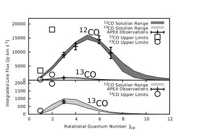
Figure 7: Top: Integrated flux densities of ¹²CO and ¹³CO transitions in the central region (18^′′ in diameter) of Circinus. We plot the solution range of ¹²CO (dark gray) and ¹³CO (light gray) derived from single-component LVG modeling of CO and ¹³CO lines with $J\geq$3. The range is selected from all solutions satisfying $\chi^{2}_{\rm red}$ $<$1.5 (or Likelihood $L>0.6$). We plot ¹²CO $J=2\rightarrow 1$, ¹²CO $J=1\rightarrow 0$, and their ¹³CO isotopic transitions for beam sizes $>$18^′′ as upper limits (black boxes and circles) to our models. Bottom: The integrated flux densities of ¹³CO, in a zoomed in view.

Table 6: CO detections toward the central position of Circinus in the literature

Transition	Telescope	Resolution	$W_{\rm mb}$	Flux	$\eta_{\rm mb}$
		(′′)	K km s-1	Jy km s-1
12CO $J=1\rightarrow 0$a	SEST	43′′	128$\pm$1.2	2650	0.77
12CO $J=1\rightarrow 0$b	SEST	41′′	185$\pm$15	3350	0.67
12CO $J=1\rightarrow 0$c	MOPRA	45′′	145	–	–
12CO $J=1\rightarrow 0$d	SEST	45′′	156	3050	0.72
12CO $J=1\rightarrow 0$e	SEST	45′′	180 $\pm$10	3500	–
12CO $J=1\rightarrow 0$f	SEST	45′′	150 $\pm$30	2850	0.7
Adopted	–	45′′	180 $\pm$10	3500	–
13CO $J=1\rightarrow 0$a	SEST	43′′	11.2$\pm$0.2	230	0.77
13CO $J=1\rightarrow 0$b	SEST	43′′	11 $\pm$1.5	210	0.68
13CO $J=1\rightarrow 0$d	SEST	45′′	13	250	0.72
13CO $J=1\rightarrow 0$e	SEST	45′′	12 $\pm$ 1	230	–
Adopted	SEST	45′′	11.2	230	–
12CO $J=2\rightarrow 1$d	SEST	45′′	125	12300	0.6
12CO $J=2\rightarrow 1$e	SEST	22′′	220$\pm$20	5400	0.6
12CO $J=2\rightarrow 1$g	SEST	38′′	177	13000	0.6
Adopted	SEST	45′′	144	14200i	–
13CO $J=2\rightarrow 1$d	SEST	45′′	12.5	1280	0.60
13CO $J=2\rightarrow 1$e	SEST	22′′	24$\pm$4	590	0.6
13CO $J=2\rightarrow 1$g	SEST	38′′	19	1390	0.6
Adopted	SEST	45′′	12.5	1300	–
12CO $J=3\rightarrow 2$d	SEST	45′′	70	20400	0.33
12CO $J=3\rightarrow 2$e	SEST	15′′	230$\pm$20	7400	0.33
12CO $J=3\rightarrow 2$g	APEX	45′′	140$\pm$20	25000	0.73
Adopted	APEX	45′′	140$\pm$20	25000	–
12CO $J=4\rightarrow 3$h	NANTEN-2	38′′	58	12600	0.5
12CO $J=3\rightarrow 2$g	APEX	45′′	80$\pm$15	25000	0.6
Adopted	APEX	45′′	80$\pm$15	25000	–

a) Aalto et al. 1991; b) Israel et al. 1992; c) Elmouttie et al. 1997 d) Curran et al. 1998; e) Curran et al. 2001a; f) Curran et al. 2001b; g) this work; h) Hitschfeld et al. 2007. i) We adopt the CO $J$=2$\rightarrow$1 to 1$\rightarrow$0 line ratio in the 45^′′ region, and the integrated intensity of ¹²CO $J=1\rightarrow 0$ in (Curran et al., 2008).

The line fluxes are derived from $T_{\rm A}^{\star}$ by adopting the telescope efficiencies of the SEST with 27 Jy/K, 41 Jy/K, and 98 Jy/K at 115 GHz, 230 GHz, and 346 GHz, respectively. For the NANTEN-2 4 m telescope, a Jy/K factor for $T_{\rm mb}$ of 216 has been assumed.

4.2.2 The CO ladder in the central 18^′′

In Fig. 7 we show the observed CO spectral line energy distribution (SLED; velocity integrated flux density versus rotational transition number $J$) and our modeled SLED for the central 18^′′ region. We also plot the line fluxes of the lower CO transitions (¹²CO $J=1\rightarrow 0$ and 2 $\rightarrow$ 1) and their ¹³C isotopic lines as upper limits. For all successful models, the ¹²CO SLEDs peak at ¹²CO $J$ = 5$\rightarrow 4$, which cannot be observed with ground-based telescopes because of the very low atmospheric transmission at this frequency.

With five observational points and three fitting parameters, our modeling has two degrees of freedom (dof), so we discuss the general properties of the set of solutions satisfying $\chi^{2}_{\rm red}$  =$\chi^{2}/({\rm dof}-1)\leq 1.5$, where $\chi^{2}_{\rm red}$  is the reduced $\chi^{2}$ . This corresponds to a likelihood limit of $L>0.6$. $L$ is defined by

$$L_{\rm i}=\exp(-\chi^{2}_{\rm i}/2)/L_{\rm max},$$ (1)

where $L_{\rm max}$ is the maximum likelihood for all solutions, which corresponds to the solution with the smallest value of $\chi^{2}$ . The best fitting result has a $\chi^{2}_{\rm red}$  of 0.5, indicating that our adopted calibration error may be a bit conservative or that the number of degrees of freedom is not large enough to reach a lower limit of exactly unity (see Andrae et al., 2010).

The best fitting result (Table 7) indicates average physical conditions of $n_{\mathrm{H}_{2}}$ $\sim$ 10^3.2cm^-3 , $T_{\rm kin}$  $\sim$ 200 K, and ${\rm d}\varv/{\rm d}r$ $\sim$ 3 km s^-1pc^-1. Various sets of degenerated parameter combinations satisfy $\chi^{2}_{\rm red}$ $<$ 1.5, and these solutions also provide reasonable fittings. The degeneracy not only affects $T_{\rm kin}$ and $n_{\mathrm{H}_{2}}$, but also ${\rm d}\varv/{\rm d}r$. For example, the “dense solution” has $n_{\mathrm{H}_{2}}$ = 10^3.7 cm^-3 , $T_{\rm kin}$ = 125 K, and ${\rm d}\varv/{\rm d}r$ = 20.0 km s^-1pc^-1, with a $\chi^{2}_{\rm red}$  $\sim$ 1.5. A ‘hot solution” with $n_{\mathrm{H}_{2}}$ = 10^3.2cm^-3 , $T_{\rm kin}$ = 250 K, and ${\rm d}\varv/{\rm d}r$ = 5.0 km s^-1pc^-1 achieves a similar $\chi^{2}$  value. In summary, these solutions encompass a range of $10^{2.7}$cm^-3 $<$$n_{\mathrm{H}_{2}}$$<$ $10^{3.8}$ cm^-3 , 80 K$<$$T_{\rm kin}$$<$400 K, 1 km s^-1pc^-1$<$${\rm d}\varv/{\rm d}r$$<$ 25 km s^-1pc^-1.

We calculate the area filling factors ($\phi_{\rm A}$) with the ratio of the observed and the modeled line intensities, by $\phi_{\rm A}=\Sigma T_{\rm obs}(i)/\Sigma T_{\rm LVG}(i)$, where $i$ is the upper level of the transitions. We find a narrow range of $\phi_{\rm A}$ between 1.8% and 2.3%. We calculate the equivalent radius with: $r_{\rm eff}=\sqrt{\phi_{\rm A}}\ r_{\rm beam}/2$, where $\phi_{\rm A}$ is the beam filling factor, and $r_{\rm beam}$ is the physical size covered by the telescope beam. The corresponding effective emission sizes are between 10 pc and 15 pc in diameter. A detailed likelihood analysis is presented in Appendix B.

Table 7: Physical parameters of single-component fitting in the central 18^′′ region, with $\chi^{2}_{\rm red}$ $<$ 1.5.

Parameters	min	max	best fitting
$\chi^{2}_{\rm red}$	0.5	1.5	0.5
Log(Density) [cm-3 ]	2.7	3.8	3.2
Temperature [K]	80	400	200
${\rm d}\varv/{\rm d}r$[km s-1pc-1]	1.0	25	3.0
$N({\rm CO})_{\rm model}$a[$10^{19}$ cm-2 ]	3.1	7.8	4.9
$N({\rm CO})_{\rm beam\thinspace}$b[$10^{17}$ cm-2 ]	5.7	17	9.2
$N({\rm H_{2}})_{\rm beam}$  c[$10^{21}$ cm-2 ]	7.1	21	11.5
$M_{\rm H_{2}}$d[$10^{7}M_{\odot}$]	0.7	2.2	1.3
Area Filling Factor ($\phi_{\rm A}$)	1.8%	2.3%	1.9%

a) $N({\rm CO})_{\rm model}$ is the CO column density derived in the LVG models.

b) $N({\rm CO})_{\rm beam}$ is the CO column density diluted by the area filling factor ($\phi_{\rm A}$).

c) $N({\rm H_{2}})_{\rm beam}$ is the beam average $\rm H_{2}$ column density.

d) $M({\rm H_{2}})$ is the molecular gas mass within a beam size of 18^′′, using $M_{\rm H_{2}}=1.36\times\frac{N({\rm CO})_{\rm beam}}{x_{\rm CO}}\times(\pi r^{2}$), where $r$ is the radius of the beam, 180 pc, and $x_{\rm CO}$ is the CO to H₂ abundance, $8\times 10^{-5}$ (Frerking et al., 1982). The helium mass is included in $M({\rm H_{2}})$. We also examined the molecular gas mass using a $R_{1213}$ of 89, which gives a range from $0.7\times 10^{7}$ M_⊙ to $2.6\times 10^{7}$ M_⊙, and the best-fit molecular gas mass is $1.7\times 10^{7}$M_⊙.

4.3 Two-component modeling in the central 45^′′ region

In this section, we explore the physical conditions in the central 45^′′ (900 pc) region with LVG modeling. We combine our mid-$J$ CO measurements with the low-$J$ CO data from the literature to perform a global fitting. We convolve all CO maps to the beam size of the SEST at the frequency of ¹²CO $J=1\rightarrow 0$, i.e., FWHM=45^′′. The intensity and resolution of these lines are tabulated in Table 6. We convolve the ¹³CO $J=3\rightarrow 2$ emission to a resolution of 45^′′, assuming that the distribution of ¹³CO $J=3\rightarrow 2$ is the same as that of ¹²CO $J=3\rightarrow 2$.

We tried to fit CO ladders in the central 45^′′ with a single LVG component first, however, it does not produce a good fit. This is not surprising since the modeling results in previous studies (e.g., Kamenetzky et al., 2012; Hailey-Dunsheath et al., 2012; Rigopoulou et al., 2013) have shown that the coexistence of multiple excitation gas components in nearby galaxies (also see Lu et al., 2014). Therefore, we use two LVG components to model the gas excitation in the central 45^′′ region.

In the two-component LVG modeling, we assume that both components have the same chemical abundance: $x_{\rm CO}$ $=8\times 10^{-5}$, and $R_{1213}$ = 40. Each component has its own $n_{\mathrm{H}_{2}}$, $T_{\rm kin}$, ${\rm d}\varv/{\rm d}r$, and a relative contribution to the measured line intensities. We list the priors in the two-component models in Table 8.

We analyze with the same grids as in the single-component fitting (see Sect. 4.2) and model the line intensities for both components simultaneously. We assume that the two-components have independent excitation conditions. The sum of the two-components should match the observed SLED. To construct the contributions of the two-components, we assume that the LE and the higher-excitation (HE) components are diluted by the filling factors of $\phi_{\rm LE}$ and $\phi_{\rm HE}$, respectively. The observed main beam temperature can be modeled with: $T_{\rm obs}$ = $T_{\rm LE}\times\phi_{\rm LE}$+ $T_{\rm HE}\times\phi_{\rm HE}=C\times[(1-R)\times T_{\rm LE}+R\times T_{\rm HE}]$, where $C$ (= $\phi_{\rm LE}+\phi_{\rm HE}$) is a constant number for each model, and $T_{\rm LE}$ and $T_{\rm HE}$ are the modeled line intensities for the low- and high- excitation components, respectively. The relative ratio $R$ ($=\frac{\phi_{\rm HE}}{\phi_{\rm HE}+\phi_{\rm LE}}$, and $0<R<1$) reflects the contribution relative to the total line intensity, and $R$ is calculated from 5% to 95% with a step size of 5%. The relative mass contributions of these phases can be expressed by: $M_{\rm H_{2}(LE)}/M_{\rm H_{2}(HE)}=\phi_{\rm LE}/\phi_{\rm HE}\times(T_{\rm LE}/T_{\rm TE})\times[X_{\rm CO(LE)}/X_{\rm CO(HE)}]$, where $X_{\rm CO(LE,HE)}$ are the $X_{\rm CO}$ factors for those phases (Papadopoulos et al., 2012a):

$$X_{\rm CO}=\frac{3.25}{\sqrt{\alpha}}\frac{n(\rm H_{2})}{T_{\rm b}(J=1\rightarrow 0)}K_{\rm vir}^{-1}(\rm\frac{M_{\odot}}{K\thinspace km\thinspace s^{-1}\thinspace pc^{2}}),$$

where $\alpha$ = 0.55 – 2.4, depending on the assumed cloud density profile, $T_{\rm b}(J=1\rightarrow 0)$ is the brightness temperature of ¹²CO $J=1\rightarrow 0$.

With nine measurements and seven fitting parameters, we discuss the general properties of the set of solutions satisfying likelihood $L$ $\geq 0.7$. In Fig 8 we plot the line flux ranges of all the accepted solutions. For all good solutions, the ¹²CO $J=1\rightarrow 0$ and $2\rightarrow 1$ intensities of the LE component are much higher than those of the HE component. The ¹²CO $J=3\rightarrow 2$ and $4\rightarrow 3$ intensities profit by similar contributions from both components. The ¹²CO $J=6\rightarrow 5$ and $7\rightarrow 6$ emission are dominated by the HE component.

We find that in the solutions with the lowest $\chi^{2}$, the relative contribution ratio is $R$ $\sim$ 0.15. Setting this ratio as the basis for the two-components, we probe the ranges of physical parameters in the following analysis. The best-fit model shows a HE component of $T_{\rm kin}$ $\sim$ 60 K, $n_{\mathrm{H}_{2}}$ $\sim$ $10^{4.2}$cm^-3 , and ${\rm d}\varv/{\rm d}r$ $\sim$ 50 km s^-1pc^-1, and a LE component of $T_{\rm kin}$ $\sim$ 30 K, $n_{\mathrm{H}_{2}}$ $\sim$ $10^{3.0}$ and ${\rm d}\varv/{\rm d}r$ $\sim$ 6 km s^-1pc^-1(for details, see Appendix C). The best fit shows an equivalent emission radius of $\sim$20 pc for the HE component, which is larger than the effective emission radius of 10–15 pc found in the previous single-component fitting.

The best solutions show that the HE component model has a velocity gradient about 10 times higher than the LE component. This indicates that more violent kinematics are associated with the HE component, and that the molecular gas in the inner 18^′′ region (Sect. 4.2.2) is in a state of high excitation because a high ${\rm d}\varv/{\rm d}r$ is expected in the center (e.g., Tan et al., 2011). We summarize the results of the two-component fittings in Table 9. Although we obtain a lower temperature, the best density solution of the LE component is also similar to the fitting results of the low-$J$ transitions of CO in Curran et al. (2001), where they find T_kin= 50-80 K, $n_{\rm H2}=2\times 10^{3}$ cm^-2 , and ${\rm d}\varv/{\rm d}r$= 10 km s^-1pc^-1.

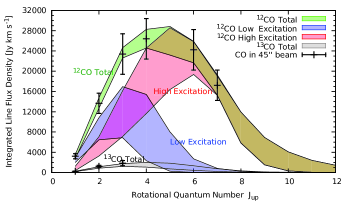
Figure 8: Integrated flux densities of ¹²CO and ¹³CO in the central 45^′′ region of the Circinus galaxy. The shadowed regions are the ranges of the best fitting results derived from the two-component LVG modeling. The high- and low- excitation components and the total integrated ¹²CO flux densities are plotted in red, blue, and green. The total integrated ¹³CO flux densities are plotted in gray.

Table 8: Parameter restrictions for the two-component LVG modeling.

1) $T_{\rm kin}$ = 10 – 1000 K

2) $n$(H2) = 102 – 107 cm-3

3) 1 $\leq$ ${\rm d}\varv/{\rm d}r$$\leq$ 360 km s-1pc-1a, $x_{\rm CO}$  = 8 $\times$ 10-5

4) $K_{\rm vir}$$>$ 1

5) M${}_{\rm H2}<$ M${}_{dyn}=3.6\times 10^{9}$M⊙b

6) $\phi_{\rm A}<1^{c}$

a) ${\rm d}\varv/{\rm d}r$ limit from Sect.  3.2.2.

b) $M_{\rm dyn}$ is the dynamical mass, $M_{\rm dyn}=3.6\times 10^{9}$M_⊙  for a beam size of 45^′′ (see Sect.  3.2.2).

c) $\phi_{\rm A}$ are area filling factors for both components derived by LVG modeling.

Table 9: Physical parameters of two-component fitting in the central 45^′′ region.

Parameter	Low-Excitation Component			High-Excitation Component
	min	max	best fitting	min	max	best fitting
Density [cm-3 ]	$10^{2.8}$	$10^{3.5}$	$10^{3.0}$	$10^{3.3}$	$10^{5.3}$	$10^{4.2}$
Temperature [K]	20	80	30	40	400	60
dv/dr [km s-1pc-1]	5	25	6	3	300	50
$N{\rm(CO)}_{\rm beam}$[$10^{17}$ cm-2 ] a	2.7	5.0	3.9	0.9	2.3	1.4
$N{\rm(CO)}_{\rm model}$[$10^{19}$ cm-2 ] b	0.9	1.5	1.2	1.5	4.6	2.3
$M_{\rm H_{2}}$ [$\rm 10^{7}M_{\odot}$] c	4.3	8.6	6.6	1.2	4.0	2.3
Filling Factor	2.6%	4.4%	3.3%	0.44%	0.82%	0.58%

a) $N{\rm(CO)}_{\rm beam}$ is the CO column density diluted by the filling factor ($\phi_{\rm A}$). b) $N{\rm(CO)}_{\rm model}$ is the CO column density derived in the LVG models. c) $M_{\rm H_{2}}$ is calculated with the beam size of 45^′′, using $M_{\rm H_{2}}=1.36\times\frac{N{\rm(CO)}_{\rm beam}}{x_{\rm CO}}\times(\pi r^{2}$), where $r$ is the radius of the beam, 450 pc. $x_{\rm CO}$ is the CO to H₂ abundance ratio, $8\times 10^{-5}$ (Frerking et al., 1982). The helium mass is included in $M\rm_{H_{2}}$.

4.4 Does the HE component arise from the 18^′′ region?

Single LVG component fitting of the inner 18^′′ region leads to an order of magnitude lower density and four times lower temperature than the corresponding parameters derived from the HE component in the 45^′′ region. If the inner 18^′′ dominates the HE component, why are there such large discrepancies? Does the HE component mainly arise from the 18^′′ region? First, the HE component in the 45^′′ region cannot entirely arise from the 18^′′ nuclear region because the ring contributes about 35% and 45% fluxes of ¹²CO $J=6\rightarrow 5$ and 7 $\rightarrow$ 6, respectively (see Sect. 4.5). Second, the single LVG component modeling only reflects the average physical conditions in this region, where the gas may not be dominated by the HE component. In the 18^′′ region the mid-$J$ transitions (especially ¹²CO $J=3\rightarrow 2$ and 4 $\rightarrow$ 3) are also likely contaminated by the lower excitation component, which may provide a large amount of diffuse cold gas along the line of sight. Third, the degeneracies between temperature, density, and velocity gradient are responsible for the difference. A component with lower density and higher temperature can produce similar CO SLEDs to a component with higher density but lower temperature.

4.5 Gas excitation in the S-F ring

For the ¹²CO $J$=6$\rightarrow$5 and $J$=7$\rightarrow$6 transitions, we find that about 35% - 45% of the CO fluxes come from the S-F ring region (diameter = 18^′′ – 45^′′), and the rest comes from the center. This indicates that the HE component derived in the two-components decomposition is not likely from the nuclear region alone, and a large amount of highly excited gas seems to exist in the S-F ring.

Benefiting from the mapping observations, we derive CO emission in the S-F ring region by subtracting line fluxes, which were derived from the best model obtained in Sect. 4.2, in the central 18^′′ region from those in the 45$"$ region. We fit the CO residual with two LVG components, to model the gas excitation exclusively in the S-F ring region, as can be seen in Fig 9. We fit the model with all transitions of ¹²CO and ¹³CO $J=1\rightarrow 0$, 2 $\rightarrow$ 1. Because ¹³CO $J=3\rightarrow 2$ was not measured in the S-F ring region, we cannot make any constraint on it. The $J$=1$\rightarrow$0 and 2$\rightarrow$1 transitions are derived from the residual by subtracting the LVG model in the central 18^′′ region from the fluxes in the 45^′′ region. The best fit of the ring shows a HE component of $n_{\mathrm{H}_{2}}$ $\sim$ 10^4.1 cm^-3 , $T_{\rm kin}$$\sim$ 125 K, and an LE component of $n_{\mathrm{H}_{2}}$ $\sim$ 10^2.9 cm^-3 , $T_{\rm kin}$$\sim$ 30 K, as shown in Table 10.

Table 10: Physical parameters of two-component fitting of the S-F ring at diameter 18^′′ $<D<$ 45^′′, with Likelihood $L>0.8$ (see Eq. 1).

Parameter	Low-Excitation Component			High-Excitation Component
	min	max	best fitting	min	max	best fitting
Density [cm-3 ]	$10^{2.9}$	$10^{3.6}$	$10^{3.2}$	$10^{3.0}$	$10^{5.0}$	$10^{4.1}$
Temperature [K]	15	40	20	15	300	60
dv/dr [km s-1pc-1]	6.0	40	10	8.0	160	40
$N{\rm(CO)}_{\rm beam}$[$10^{17}$ cm-2 ] a	2.2	4.2	3.7	0.3	1.6	0.6
$N{\rm(CO)}_{\rm model}$[$10^{19}$ cm-2 ] b	0.7	1.5	1.2	1.5	4.6	2.3
$M_{\rm H_{2}}$ [$\rm 10^{7}M_{\odot}$] c	3.8	7.5	6.4	0.6	2.3	1.0
Filling Factor ($\phi_{\rm A}$)	2.4 %	4.6%	3.2%	0.17%	0.35%	0.24%

a) $N{\rm(CO)}_{\rm beam}$ is the CO column density diluted by the filling factor ($\phi_{\rm A}$). b) $N{\rm(CO)}_{\rm model}$ is the CO column density derived in the LVG models. c) $M_{\rm H_{2}}$ is calculated with $M_{\rm H_{2}}=1.36\times\frac{N{\rm(CO)}_{\rm beam}}{x_{\rm CO}}\times(\pi r^{2}$), where $r$ is the effective radius of the beam, $r=\sqrt{(450^{2}-180^{2})}=$ 412 pc. $x_{\rm CO}$  is the CO to H₂ abundance, $8\times 10^{-5}$ (Frerking et al., 1982). The helium mass is included in $M\rm_{H_{2}}$ by adopting a factor of 1.36.

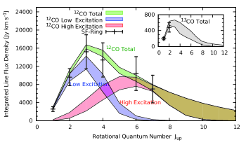
Figure 9: Integrated flux densities of ¹²CO and ¹³CO in the S-F ring region of the Circinus galaxy. The shadowed regions are the ranges of the fittings satisfying likelihood $L>0.8$, derived from the two-component LVG modeling. The high- and low- excitation components and the total integrated ¹²CO flux densities are plotted in red, blue, and green. The total ¹³CO flux densities are plotted in gray.

4.6 Comparison with NGC 1068

Circinus and NGC 1068 have many similarities. They are both nearby Seyfert galaxies, which contain gas-rich nuclei and molecular S-F rings. Although Circinus has a much smaller distance ($\sim$ 4 Mpc) than NGC 1068 ($\sim$ 14.4 Mpc Bland-Hawthorn et al., 1997), the angular sizes of the gas-rich region in these two galaxies are both about 40^′′ (in diameter). Both of them have strong S-F activities in their centers, and are fed by large amounts of molecular material (e.g., Curran et al., 2001; Hailey-Dunsheath et al., 2012).

In NGC 1068, the inner ends of the S-F spiral arms lead to a large S-F ring of diameter $\sim$2.3 kpc (e.g., Schinnerer et al., 2000; Gallimore et al., 2001). Closer to the center there is a circumnuclear disk (CND) of diameter $\sim$300 pc, seen most prominently in line emission of dense gas tracers (e.g., Schinnerer et al., 2000; Krips et al., 2011). Between the S-F ring and the CND there is a gap region deficient in molecular gas (e.g., Helfer et al., 2003; Schinnerer et al., 2000; Tacconi et al., 1997; Tsai et al., 2012). Spinoglio et al. (2012) modeled the excitation conditions with the CO SLED deduced from the Herschel observations and found an LE component ($T_{\rm kin}$ $=$ 120 K, $n_{\mathrm{H}_{2}}$ $=$ 10^2.8cm^-3 ) associated with an extended source (the S-F ring), a medium excitation (ME) component ($T_{\rm kin}$$=$ 100 K, $n_{\mathrm{H}_{2}}$ $=$ $10^{4.6}$ cm^-3 ) associated with the CND, and a HE component ($T_{\rm kin}$$=$ 150 K, $n_{\mathrm{H}_{2}}$ $=$ $10^{5.7}$ cm^-3 ) possibly arises from the central few pc heated by the AGN (e.g., Hailey-Dunsheath et al., 2012).

Considering the whole inner 45^′′ region of Circinus, the LE component has $n_{\mathrm{H}_{2}}$ $\sim 10^{3.0}$ cm^-3 , similar to the LE component derived from the extended emission in NGC 1068 and the central region of the Milky Way (e.g., Spinoglio et al., 2012; Ott et al., 2014). The temperature of the LE component, however, is $T_{\rm kin}$  $\sim$ 30 K, which is much lower than the LE component in NGC 1068, indicating that Circinus may have lower excitation conditions.

On the other hand, the HE component in Circinus is also characterized by a similar density and a lower temperature compared to the ME component in NGC 1068, which is from the CND region, and s fitted using the high-$J$ transitions ($J$=9$\rightarrow$8 to 13$\rightarrow$12) in a 17^′′ region (i.e., Spinoglio et al., 2012). The velocity gradient of the HE component spans a large range and all solutions indicate that this gas component is in a highly supervirialized state.

In NGC 1068, the LVG modeling was made step by step from higher to lower excitation components. Each component was fitted individually, after subtracting the higher excitation components. In Circinus we fit the two-components simultaneously, which allows for a much larger parameter space. The different fitting methods could also introduce differences. High angular resolution observations of multiple-$J$ CO transitions in Circinus are needed to fully resolve the gas phase distribution and fully test the above scenarios.

4.7 Molecular gas mass

We calculate molecular gas mass from the LVG models derived from previous sections. RADEX gives the column density $N_{\rm CO}$ without beam dilution. We convert it to a beam-averaged ¹²CO column density $<N_{\rm CO}>$, which is then further converted to the column density of molecular hydrogen with the assumed CO abundance of $x_{\rm CO}$  $=8\times 10^{-5}$. The molecular gas mass is derived with

$$M_{H_{2}}=1.36\times m_{H_{2}}\frac{<N_{\rm CO}>}{x_{\rm CO}}\frac{\int{T_{\rm mb}}{dv}\times A}{W},$$ (2)

where $m_{H_{2}}$ is the mass of a single H₂ molecule and the factor of 1.36 accounts for the mass of helium in the molecular clouds. The beam area $A=\pi\ r_{0}^{2}$, where $r_{0}$ is radius of the beam. The velocity integrated line intensity $W$ is calculated in the LVG models. The main beam temperature $T_{\rm mb}$ is obtained from the observations (Ward et al., 2003).

In the single-component modeling, the beam size corresponds to a region with radius $r_{0}$ of (central) 180 pc. From the best fitting results (see Sect. 4.2), a velocity gradient ${\rm d}\varv/{\rm d}r$ $\sim$ 3 km s^-1pc^-1, and a density $n_{\mathrm{H}_{2}}$ $\sim$ 10^3.2 cm^-3  are used. We derived a molecular gas mass of 1.3$\rm\times 10^{7}\ M_{\odot}$, and an area filling factor of $\sim$ 2%.

The two-component fitting refers to a region of 45^′′ in radius, which corresponds to a radius of 450 pc. The total molecular gas mass is derived to be 8.9$\rm\times 10^{7}M_{\odot}$ for the best-fit result, which contains a gas mass of 6.6 $\times 10^{7}M_{\odot}$ for the LE component, and 2.3 $\times 10^{7}$M_⊙ for the HE component.

The molecular gas mass in Circinus has been debated for a long time. Using the 1.3 mm continuum, Siebenmorgen et al. (1997) derived a molecular gas mass of 1.6 $\times 10^{8}$ M_⊙ within their $3^{\prime}\times 4^{\prime}$ maps of the central region of Circinus. From the Galactic disk standard conversion factor ($2\times 10^{20}\rm$ $({\rm Kkms}^{-1})^{-1}$; Strong et al. 1988; Bolatto et al. 2013), the molecular gas mass derived from ¹²CO $J=1\rightarrow 0$ reaches $1.6\times 10^{9}$M_⊙ in the central 560 pc (e.g., Elmouttie et al., 1997; Curran et al., 1998). This would indicate that the molecular gas mass constitutes half of the dynamical mass in the central 560 pc region, which is more than the molecular gas mass fractions in most luminous galaxies and nuclear regions of normal S-F galaxies (e.g., Young & Scoville, 1991; Sakamoto et al., 1999). Hitschfeld et al. (2008) performed both Local Thermal Equilibrium (LTE) and LVG analysis with the lowest four transitions of CO and the C i transition. They found that the column densities of CO are about 4–7 $\times 10^{17}$ cm^-2 in the central 560 pc region, and this is $\sim 1/10$ of the column density ($N_{\rm CO}=3\times 10^{18}$ cm^-2 ) derived from the standard conversion factor. This evidence implies that the standard conversion factor in Circinus is ten times lower than the Galactic disk value (e.g., Dahmen et al., 1998; Bell et al., 2007; Israel, 2009a, b; Bolatto et al., 2013)

The best fitting in our two-component LVG modeling gives a total molecular gas mass of $\sim 9\times 10^{7}$M_⊙ in the central 45^′′ region, which corresponds to a standard conversion factor of $N({\rm H_{2}})/I_{\rm COJ=1\rightarrow 0}=$ $0.37\times 10^{20}$ cm^-2 $({\rm K\ km\ s}^{-1})^{-1}$ (for $x_{\rm CO}$  $=8\times 10^{-5}$ used here). The molecular gas mass determined from LVG modeling is about 60% of the mass of 1.6$\times 10^{8}$ M_⊙ derived by the 1.3 mm continuum obtained in a larger region (Siebenmorgen et al., 1997). Mauersberger et al. (1996), Downes & Solomon (1998), Papadopoulos & Seaquist (1999), Israel (2009a), and Bolatto et al. (2013) also derived conversion factors significantly lower than the Galactic value by analyzing the low-$J$ CO emission in NGC 1068 and other galaxies with bright CO emission and high stellar surface density. This suggests that the lower conversion factor likely arises from gas being not virialized (e.g., Aalto et al., 1995; Dahmen et al., 1998; Narayanan et al., 2011).

4.8 Molecular gas mass estimates using C i 

Atomic carbon (C i) could help circumvent the problem of defining a proper conversion factor because its emission traces molecular gas independently. The critical density of C i is $\approx$ 1 $\times 10^{3}$ cm^-3 (e.g., Tielens, 2005), similar to that of ¹²CO $J$=1$\rightarrow$0, thus provides approximate thermalization at the densities reported here (see Tables 7, 9, and 10). Strong evidence shows that C i and CO luminosities have a tight correlation in galaxies, independent of physical environment, IR luminosity, or redshift (e.g., Papadopoulos & Greve, 2004; Zhang et al., 2007; Walter et al., 2011). This suggests that C i emission arises from the same volume and shares similar excitation temperature as CO (e.g., Ikeda et al., 2002). Constant ratios between the column densities of C i, ¹²CO, and H₂ are expected over a large range of physical conditions (e.g., Papadopoulos & Greve, 2004; Walter et al., 2011).

Constraining H₂ column density with the optically thin C i lines is an independent and robust way to probe the molecular gas mass in galaxies. We can calculate the mass of C i following Weiß et al. (2005):

$$M({\rm CI})=1.9\times 10^{-4}Q(T_{\rm ex}){\rm e}^{23.6/T_{\rm ex}}L^{\prime}({\rm CI}\ ^{3}P_{1}\rightarrow^{3}P_{0})[{\rm M}_{\odot}],$$

where $Q({{T}_{\rm ex}})=1+3{\rm e}^{-T_{1}/{{T}_{\rm ex}}}+5{\rm e}^{-T_{2}/{{T}_{\rm ex}}}$ is the C i partition function, and $T_{1}$ = 23.6 K and $T_{2}$ = 62.5 K are the energies above the ground state. The [C i]/[H2] abundance chosen here is $x_{\rm C_{\rm I}}=5\times 10^{-5}$ (Weiß et al., 2005). We adopt an excitation temperature of 30 K derived from the LE component in the two-component LVG fittings (Table 9). Assuming $T_{\rm ex}$ = $T_{\rm kin}$= 30 K, we derive a molecular gas mass of 8.3$\times 10^{7}$ M_⊙. If $T_{\rm ex}$= 60 K from the HE component is adopted, the molecular gas mass is 8.9 $\times 10^{7}$ M_⊙. These masses are, within the errors, consistent with the result derived from our LVG solution, 9 $\times$ 10⁷ M_⊙ (Sect. 4.7).

4.9 Luminosities of C i and ¹²CO $J=3\rightarrow 2$ 

In Fig. 2, we present the spectra of C i and ¹²CO $J=3\rightarrow 2$ observed in the central region of Circinus. The line profiles of the two species are similar. In the following, we calculate the line luminosities ($L^{\prime}_{\rm line}$) of CO and C i, and compare them with nearby galaxies and high-$z$ systems. We determine the line luminosity following the definition in Solomon et al. (1992):

$$\frac{L^{\prime}_{\rm line}}{\rm(Kkms^{-1}pc^{2})}=3.25\times 10^{7}S_{\rm line}\Delta\varv\nu_{\rm obs}^{-2}D_{L}^{2}(1+z)^{-3},$$ (3)

where $L^{\prime}$ is the line luminosity in K km s^-1  pc², $S_{\rm line}\Delta\varv$ is the velocity integrated flux density in Jy km s^-1 , $D_{\rm L}$ denotes the luminosity distance in Mpc, and $\nu_{\rm obs}$ represents the observing frequency in GHz. The $L^{\prime}_{\rm line}$ ratios stand for ratios of the intrinsic brightness temperatures.

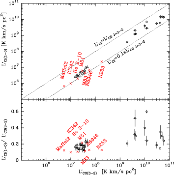
Figure 10: $L^{\prime}\rm_{\rm CI}$ as a function of $L^{\prime}\rm_{\rm CO\ J=3\rightarrow 2}$. The empty triangles show observed positions in Circinus. The empty circles show the galaxies at high redshift (Walter et al., 2011). The crosses represent results of nearby galaxies found in literature. NGC 6946 and M 83: (Israel & Baas, 2001), M 51: (Israel et al., 2006), Hennize 2-10 and NGC 253: (Bayet et al., 2004), IC 342: (Israel & Baas, 2003).

In Fig. 10, we plot the C i line luminosity as a function of ¹²CO $J=3\rightarrow 2$ luminosity. We combined the C i data from the literature, including the C i detections in nearby and high-redshift galaxies (e.g., Walter et al., 2011). The luminosities of C i and ¹²CO $J=3\rightarrow 2$ match each other and the scatter of the ratios lies within an order of magnitude (the dashed diagonal lines). The correlation derived from multiple position in Circinus basically follows the same trend found in high-redshift galaxies.

We find that the C i to ¹²CO $J=3\rightarrow 2$ luminosity ratios $R_{\rm CI/CO32}$ in nearby galaxies (red crosses) are lower than those found in the high-redshift galaxies and the AGN hosting galaxies (i.e., Circinus and M 51). An average ratio of $R_{\rm CI/CO32}$ = 0.17$\pm$0.03 is found in Circinus, and this is only about half of the average ratio found at highredshift (Walter et al., 2011, $0.32\pm 0.13$). In the quiescent nearby galaxies, $R_{\rm CI/CO32}$ are mostly close to 0.1. In the central positions of M 51 and Circinus, the $R_{\rm CI/CO32}$ ratios are both $\sim 0.2$, about two times higher than those in quiescent galaxies. These high $R_{\rm CI/CO32}$ ratios are likely caused by the enhanced gas excitation due to the AGN activities.

5 Summary and conclusions

We present new APEX mapping observations of ¹²CO $J=3\rightarrow 2$, $4\rightarrow 3$, $6\rightarrow 5$, $7\rightarrow 6$ and C i 1$\rightarrow$0 in the central region of the Circinus galaxy. These data are to date the highest transitions published. All these lines reveal extended strong emission and similar kinematic structures. We find strong ¹²CO $J=6\rightarrow 5$ and $7\rightarrow 6$ emission not only in the nuclear region, but in the gas-rich, star-forming (S-F) ring region at galactocentric diameter of $18^{\prime\prime}<D<45^{\prime\prime}$ as well. The latter region contributes about 35%-45% of the measured high-$J$ CO emission. With the CO maps we are able to decompose the gas excitation spatially.

By using radiation transfer analysis we find two distinct areas with different gas excitation conditions: the $18^{\prime\prime}$ nuclear region and the S-F ring within $18^{\prime\prime}<R<45^{\prime\prime}$. Our main results are as follows:

1) With a single excitation component, we use APEX ¹²CO and ¹³CO detections ($J\geq 3$) to perform a LVG modeling. We derive $n_{\mathrm{H}_{2}}$ $\sim$ $10^{3.2}$cm^-3 , $T_{\rm kin}$$\sim 200$K, ${\rm d}\varv/{\rm d}r$$\sim$ 3.0 km s^-1pc^-1, and $M_{\rm H_{2}}\sim 1.3\times 10^{7}$M_⊙ in the central 18^′′ region, which accounts for $\sim$ 15% of the total molecular gas mass in the central gas-rich 45^′′ region in Circinus.

2) Combined with low-$J$ CO data in the literature, we perform two-component LVG modeling in the central 45^′′ diameter region, and in the S-F ring. We find two excitation components that can fit the measurements in the whole region, one with $n_{\mathrm{H}_{2}}$ $\sim$ $10^{3.0}$cm^-3 , $T_{\rm kin}$$\sim 30$K, ${\rm d}\varv/{\rm d}r$$\sim$ 6 km s^-1pc^-1, and $M_{\rm H_{2}}\sim 6.6\times 10^{7}$M_⊙, and the other with $n_{\mathrm{H}_{2}}$ $\sim$ $10^{4.2}$cm^-3 , $T_{\rm kin}$$\sim 60$K, ${\rm d}\varv/{\rm d}r$$\sim$ 50 km s^-1pc^-1, and $M_{\rm H_{2}}\sim 2.3\times 10^{7}$M_⊙. In the ring region, the high density component represents a smaller fraction ($\sim$13%) of the total gas mass. All these gas components are supervirialized.

3) We find the molecular gas mass of Circinus is $\sim 0.9\times 10^{8}$ M_⊙ in the 45^′′ region. This is consistent with the gas mass derived from C i ($\sim 0.9\ \times 10^{8}$ M_⊙) and is $\sim$ 60% of the gas mass obtained using submm continuum in a larger area ($1.6\times 10^{8}$ M_⊙). A gas mass of about $\sim 1.3\times 10^{7}$ M_⊙ is found in the central 18^′′ nuclear region, and $\sim 7.5\times 10^{7}$ M_⊙ is located in the surrounding ring. In the 45^′′ region, we thus derive a conversion factor of $N({\rm H_{2}})/I_{\rm COJ=1\rightarrow 0}$ = $0.37\times 10^{20}$cm^-2 $({\rm Kkms}^{-1})^{-1}$, which is about 1/5 of the Galactic disk value.

4) We find the average luminosity ratio between C i (1$\rightarrow$0) and ¹²CO $J=3\rightarrow 2$ ($R_{\rm CI/CO32}$) in Circinus to be 0.2, about twice the average value found in nearby normal galaxies (Gerin & Phillips, 2000, $\sim 0.1$). This is near the low end of what is observed in high-redshift systems (Walter et al., 2011, $\sim 0.29$).

Appendix A Virialized gas state

The gravitational potential of the densely packed stars and the nearby super massive nuclear engine in the central region of a massive galaxy may cause significant velocity gradients along lines of sight, which can be well in excess of what would be found in a normal cloud near virial equilibrium. Therefore the velocity gradient expected in the virialized gas motion can be taken as a lower limit. The ratio between the measured velocity gradient and that calculated from virial equilibrium is defined by

$$K_{\rm vir}=\frac{(dv/dr)_{\rm LVG}}{(dv/dr)_{\rm vir}}.$$ (4)

The virialized velocity gradient is given by

$$\begin{split}\left(\frac{dV}{dr}\right)_{\rm VIR}\approx\frac{\delta v_{\rm vir}}{2R}=\left(\alpha\frac{\pi G\mu}{3}\right)^{1/2}\ \langle n\rangle^{1/2}\\ \sim 0.65\alpha^{0.5}(\frac{<n>}{\rm 10^{3}\thinspace cm^{-3}})^{1/2}{\rm kms^{-1}pc^{-1}},\end{split}$$ (5)

where $\mu$ is the mean particle mass, G is the gravitational constant, $<$n$>$ is the mean number density of the cloud, and $\alpha$ is a constant between 0.5 to 3 depending on the assumed density profile (Bryant & Scoville 1996). For a cloud with assumed density of 10⁵cm^-3 , and with the largest value of $\alpha$=3, the estimated (dv/dr) is about 10 km s^-1pc^-1. For more diffuse gas with a density of 10³cm^-3  and $\alpha$=0.5, (d$v$/d$r$) is around 0.5 km s^-1pc^-1. Molecular gas close to the central massive black hole will be strongly influenced by gravity (e.g., Bonnell & Rice 2008), thus could be subvirialized ($K_{\rm vir}$ $<$ 1). However such an effect is likely obvious only within a few tenths pc in the center. On the other hand, the tidal shear produced by the black hole would also increase the instability of molecular gas, where $K_{\rm vir}$ $>$ 1.

Appendix B Likelihood analysis of the single-component fitting

In the following, we analyze possible solution ranges for the central 18^′′ of the Circinus galaxy and corresponding physical conditions satisfying maximum likelihood achievable in the set of all combinations parameters (see also Sect. 4.2.1). We caution, however, that these findings – in particular the numbers shown below – are rather uncertain, and will be only indicative.

Instead of the Bayesian probability, which is the integral of all probabilities in the parameter space (e.g., Weiß et al. 2005; Hailey-Dunsheath et al. 2012; Kamenetzky et al. 2011; Rangwala et al. 2011), we analyze the trend of the solutions with the highest likelihood. The maximum likelihood function of a given parameter (or given parameters) is based on the best fitting results in the whole parameter space.

Fig. 11 (upper panel) shows the maximum likelihood as a function of velocity gradient in a range of 1 km s^-1pc^-1$\leq$ ${\rm d}\varv/{\rm d}r$$\leq$ 10³ km s^-1pc^-1. We plot the corresponding values of $n_{\mathrm{H}_{2}}$ and $T_{\rm kin}$ of the best fit for each given velocity gradient (lower panel). Over the modeled ${\rm d}\varv/{\rm d}r$ range, $T_{\rm kin}$ and $n_{\mathrm{H}_{2}}$ vary by about an order of magnitude. The likelihood drops below half of the peak value when ${\rm d}\varv/{\rm d}r$ is beyond 10^1.8 km s^-1pc^-1, where the solutions have relative high temperature and low density. This suggests that reasonable models are not likely to have a ${\rm d}\varv/{\rm d}r$ higher than 60 km s^-1pc^-1 because then even the best fitting result shows poor fits to the measurements.

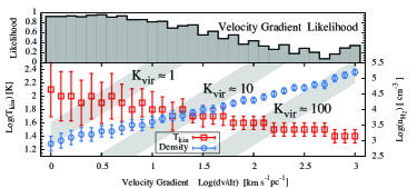
Figure 11: Upper panel: The histogram shows the maximum likelihood as a function of the velocity gradient ${\rm d}\varv/{\rm d}r$ for single-component LVG fitting. Lower panel: The best-fit values of density (blue circles) and temperature (red squares) for a given velocity gradient as functions of velocity gradient, with error bars showing a 1$\sigma$ range of the likelihood distribution. The gray regions have $K_{\rm vir}$$\sim$1, 10, and 100.

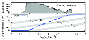
Figure 12: Upper panel: The histogram shows the maximum likelihood as a function density for single-component LVG fitting. Lower panel: The best-fit velocity gradient for a given density as a function of density. The gray regions have $K_{\rm vir}$$\sim$1, 10, and 100.

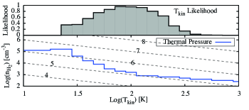
Figure 13: Upper panel: The histogram shows the maximum likelihood as a function of temperature for single-component LVG fitting. Lower panel: The best-fit density for a given temperature as a function of temperature. The dashed lines show thermal pressure, $\log$($n_{\mathrm{H}_{2}}$$\times$ $T_{\rm kin}$), in units of K cm^-3.

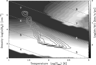
Figure 14: The contours show the distributions of the maximum likelihood for a given density and temperature in the single-component LVG fitting. Contours are drawn from 0.1 to 0.9 by 0.2. Background gray scale levels show the velocity gradient associated with the best LVG fitting results, for each given temperature and density. The dashed lines indicate the thermal pressure $\log$($n_{\mathrm{H}_{2}}$$\times$ $T_{\rm kin}$) in units of K cm^-3.

Fig. 12 shows the maximum likelihood as a function of $n_{\mathrm{H}_{2}}$ in a ${\rm H_{2}}$ density range from 10² cm^-2 to 10⁶ cm^-2 . We plot the corresponding ${\rm d}\varv/{\rm d}r$ of the best fits as a function of density. The solutions are found over a broad range of velocity gradients, which increase almost linearly as density increases. Solutions with high densities also have high velocity gradients. But the density is not likely to be higher than $10^{4.5}$cm^-3  where the likelihood is dropping below half of the peak value and $K_{\rm vir}$ exceeds ten. This implies that models with high density solutions are highly supervirialized and are not bound by self-gravity.

Fig. 13 shows the maximum likelihood as a function of $T_{\rm kin}$ from 10 K to 10³ K. The thermal pressure $P=n_{\rm H_{2}}\times T_{\rm kin}$ of the best fitting results is presented for given temperatures. The thermal pressure decreases by an order of magnitude when $T_{\rm kin}$ increases from a few tens of K to about 200 K. This indicates that the solutions of high temperature will have low thermal pressure because of the corresponding low density of these solutions.

In Fig. 14, we show as contours the density-temperature likelihood distribution of the LVG modeling. The gray scale background displays the velocity gradient associated with the best fitting results, at given temperatures and densities. The contours present a banana-shaped likelihood distribution, which is mainly caused by the degeneracy between temperature and density. In the contour map, thermal pressure almost stays constant along the ridge of the distribution. Both density and temperature vary by two orders of magnitude within the 50% contour. The likelihood distribution covers a range of thermal pressure from $10^{4.8}$ to $10^{6.5}$ Kcm^-3  and peaks at $\sim 10^{5.2}$ Kcm^-3 . From the map of the associated velocity gradients in the background, ${\rm d}\varv/{\rm d}r$ increases with $n_{\mathrm{H}_{2}}$, and decreases with $T_{\rm kin}$. Most good solutions have small ${\rm d}\varv/{\rm d}r$ between 1 km s^-1pc^-1and 10 km s^-1pc^-1.

Appendix C Likelihood analysis of the two-component fitting

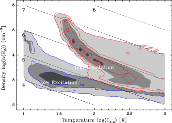
Figure 15: Background gray scale images show the maximum likelihood distributions of temperature and density, derived from the two-component LVG modelings. The gray levels are from 0.1 to 0.9 with a spacing of 0.2. The low- and high excitation components are plotted in blue and red contours. The dashed lines indicate thermal pressure, $\log$($n_{\mathrm{H}_{2}}$$\times$ $T_{\rm kin}$), in units of K cm^-3.

In Fig. 15, we show the maximum likelihood distribution of both components in our modeling, with contours of the enclosed probability. Both distributions have banana shapes that are mainly caused by the degeneracy between $T_{\rm kin}$ and $n_{\mathrm{H}_{2}}$. We find that both distributions are characterized by component specific thermal pressures. The thermal pressure of the HE component is about one order of magnitude higher than that of the LE component.

The HE component shows a steep slope in the high density and low temperature regime, and a flat slope at the high temperature side with a very broad range of $T_{\rm kin}$ solutions. This indicates that the density is not tightly constrained for the HE component. The HE component has a best-fit ${\rm d}\varv/{\rm d}r$ of $\sim$ 50 km s^-1pc^-1, which is about 10 times higher than that of the LE component, where $\sim$6 km s^-1pc^-1 is the best fitting result. General fitting results of both excitation components are listed in Table 9.

Fig. 16 shows the density likelihood as functions of both excitation components (lower panel), and the corresponding velocity gradient of the best fittings for given densities (upper panel). The higher the density, the larger the velocity gradient for both components. Solutions with higher densities also have higher $K_{\rm vir}$. Molecular gas in such conditions has very violent motions and high temperature. Unless the HE component adopt a low density solution of $\sim 10^{3.5}$cm^-3 , $K_{\rm vir}$ is always higher than unity. The density range of the HE component is much wider than that of the LE component, which is due to the high degeneracy between $n_{\mathrm{H}_{2}}$, $T_{\rm kin}$, and ${\rm d}\varv/{\rm d}r$, and less constrained for the high-$J$ transitions. In Fig. 17, the temperatures of both components are not well constrained although the likelihood curve of the LE component looks narrower and peaks at lower temperature ($\sim$ 40 K) than that of the higher temperature ($\sim$ 50 K). The thermal pressure drops when the temperature increases, and stays nearly constant when the temperatures of both components are higher than 100 K.

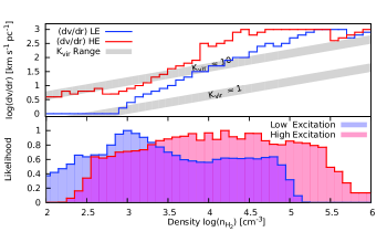
Figure 16: Upper panel: Velocity gradients of the best fitting results as functions of density, derived from the two-component LVG modeling. The gray regions have $K_{\rm vir}$$\sim$1 and 10. Lower panel: The maximum likelihood as functions of the densities of both excitation components. The low- and high- excitation components are plotted in blue and red shadows, respectively.

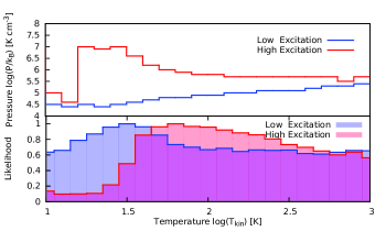
Figure 17: Upper panel: Thermal pressure ($\log$($n_{\mathrm{H}_{2}}$$\times$ $T_{\rm kin}$)) of the best fitting results as functions of density, derived from the two-component LVG modeling. Lower panel: The maximum likelihood as functions of temperatures for both excitation components. The low- and high- excitation components are plotted in blue and red shadows, respectively.