Multiple-Candidate Successive Interference Cancellation with Widely-Linear Processing for MAI and Jamming Suppression in DS-CDMA Systems

Abstract

In this paper, we propose a widely-linear (WL) receiver structure for multiple access interference (MAI) and jamming signal (JS) suppression in direct-sequence code-division multiple-access (DS-CDMA) systems. A vector space projection (VSP) scheme is also considered to cancel the JS before detecting the desired signals. We develop a novel multiple-candidate successive interference cancellation (MC-SIC) scheme which processes two consecutive user symbols at one time to process the unreliable estimates and a number of selected points serve as the feedback candidates for interference cancellation, which is effective for alleviating the effect of error propagation in the SIC algorithm. Widely-linear signal processing is then used to enhance the performance of the receiver in non-circular modulation scheme. By bringing together the techniques mentioned above, a novel interference suppression scheme is proposed which combines the widely-linear multiple-candidate SIC (WL-MC-SIC) minimum mean-squared error (MMSE) algorithm with the VSP scheme to suppress MAI and JS simultaneously. Simulations for binary phase shift keying (BPSK) modulation scenarios show that the proposed structure achieves a better MAI suppression performance compared with previously reported SIC MMSE receivers at lower complexity and a superior JS suppression performance.

I introduction

Direct-sequence code-division multiple-access (DS-CDMA) systems are one of the most successful multiple access technologies for wireless communication systems. Such services include third generation cellular telephone, indoor wireless networks and satellite communication systems. Multiple access interference (MAI), arising from the nonorthogonality between the signature sequences and jamming signals is a significant limiting factor to the performance of DS-CDMA systems. To address this problem, the optimum multiuser detector (MUD) and several suboptimum MUDs were introduced [1]. Optimal multiuser detection has an exponential computational complexity and is therefore impractical. Several low-complexity multiuser detectors including the linear decorrelator, the linear minimum mean-squared error (MMSE), the successive interference cancellation (SIC) [2], and the parallel interference cancellation (PIC) have been proposed [3].

The SIC detector regenerates and cancels the signals of other users before data detection of the desired user. The potential of SIC to alleviate the near–far problem comes from its property of removing stronger users before detecting weaker users. Specific forms of the SIC are closely related to approximations of the optimum maximum likelihood (ML) detector [4, 5], as well as iterative techniques for solving linear equations [6]. There are several variants of the SIC algorithm, which have been investigated in last decade or so [8]-[14]. The performance of the SIC algorithm relies heavily on the accuracy of the symbol estimate and is subject to error propagation effects when the estimated symbol is not accurate. Methods including soft or linear interference cancellation and partial interference cancellation are proposed to mitigate this error propagation [7]. A multiple feedback SIC (MF-SIC) algorithm with shadow area constraints (SAC) strategy for detection of multiple data streams has been introduced in [10]. The MF selection algorithm searches several constellation points rather than one and chooses the most appropriate constellation symbol as the decision. A joint successive interference cancellation technique (JSIC) has been introduced in [12]. The key idea behind JSIC is to exploit the structural properties of the sub-constellation formed by the signals of two consecutive users in an ordered set to gain an improvement in the detector performance.

In wireless communication systems, most interference suppression or parameter estimation techniques are based on linear signal processing [15, 16]. However, when a noncircular modulation is applied, e.g. binary phase shift keying (BPSK), linear estimation of an improper real-valued signal from complex data appears complex, which in a statistical signal processing sense, is not optimal. It has been shown in [24] that by exploiting the improper nature of the received signal, the estimation performance can be significantly improved. Therefore, the resulting widely linear (WL) estimate has gained great popularity for systems using non-circular modulation schemes [25, 26, 27].

The jamming signal (JS) is another form of interference which has a huge influence on the performance of DS-CDMA systems. The notch filter is used to cancel the JS and an estimate of the interference parameters is required before the interference cancellation [31]. A generalized approach for the JS suppression in PN spread-spectrum communications using open-loop adaptive excision filtering is introduced [32]. The algorithm has a tradeoff between interference removal and the amount of self-noise generated from the induced correlation across the PN chip sequence due to the filtering procedure. A new transversal filter structure is used before correlation to improve the performance of DS-CDMA systems [33]. Several subspace techniques have been developed to exploit the low-rank structure of the interference in . The eigenspace-based interference canceller has been proposed in [44] and to cancel the interference through constructing the proposed estimate-and-subtract interference cancellation beamformer.

The goal of this work is to develop an interference suppression strategy for DS-CDMA systems that operates in the presence of non-circular data, JS and MAI. To this end, we bring together a novel SIC algorithm, WL processing and a JS cancellation scheme. Inspired by the error propagation mitigation in the MF-SIC and JSIC algorithms, we propose a novel Multiple-Candidate SIC (MC-SIC) scheme which processes two consecutive user symbols at one time when the current symbol decision is not reliable and also exploits the constellation knowledge in the generation of candidates for detection. In addition to this, we combine WL processing with the MC-SIC scheme and propose a widely linear MC-SIC (WL-MC-SIC) algorithm, which aims to deal with the performance degradation due to error propagation in SIC and linear signal processing on the noncircular signal. We also devise a technique to cancel JS that is incorporated into the proposed WL-MC-SIC algorithm, which relies on a vector space projection (VSP) method. The interference cancellation operator is constructed to project the desired signal onto the complement of the JS subspace.

The main contributions of this paper are summarized as follows:

• A MC-SIC scheme based on the MMSE criterion is proposed.

• A novel widely linear MC-SIC (WL-MC-SIC) MMSE algorithm is devised, which combines WL processing and a MC-SIC MMSE scheme to improve the detector’s performance under noncircular modulation scheme and alleviate the effect of error propagation in the traditional SIC algorithm.

• A novel interference mitigation scheme is proposed which combines the VSP algorithm with the WL-MC-SIC MMSE algorithm to jointly suppress the MAI and JS.

• The performance of the proposed algorithm for MAI and JS suppression is compared with other interference suppression schemes.

The organization of the paper is as follows. The system model is given in Section II. Section III introduces the proposed WL-MC-SIC algorithm and VSP. In Section IV the complexity of the WL-MC-SIC algorithm is analyzed. Section V presents the simulation results and a comparison between the proposed WL-MC-SIC algorithm with the VSP method and previously reported algorithms.

Notation: In this paper, scalar quantities are denoted with italic typeface. Lowercase boldface quantities denote vectors and uppercase boldface quantities denote matrices. The operations of transposition, complex conjugation, and conjugate transposition are denoted by $\{\cdot\}^{T}$, $\{\cdot\}^{\ast}$ and $\{\cdot\}^{H}$, respectively. The symbol $\textrm{E}[\cdot]$ denotes the expected value of a random quantity, the operator $\mathcal{R}\{\cdot\}$ selects the real part of the argument, the operator $\mathcal{J}\{\cdot\}$ selects the imaginary part of the argument, $\mathcal{L}[\boldsymbol{M}]$ denotes a linear subspace spanned by the columns of the matrix A and the operator $|\cdot|$ denotes the absolute value of the argument.

II system model

Let us consider a synchronous DS-CDMA system with K active users signaling through an additive Gaussian noise channel. The received baseband signal during one symbol interval in such channel can be modeled as

$$\begin{split}r(t)&=\sum_{k=1}^{K}{A_{k}}{b}_{k}s_{k}(t)+j(t)+n(t),~{}~{}~{}t\in[0,T],\end{split}$$ (1)

where $j(t)$ and $n(t)$ represent the jamming signal and the ambient channel noise respectively; $T$ is the symbol interval; $b_{k}\in\{\pm{1}\}$ is the BPSK symbol for the user $k$ with amplitude $A_{k}$, and $s_{k}(t)$ is the spreading sequence waveform of the $k$-th user.

After chip matched filtering and time synchronization, sampling with rate ${L}/{T}$, where $L$ is equal to the spreading factor and appropriate normalization, the vector $\boldsymbol{r}(i)$ containing the $L$ samples received in the interval $[iT;(i+1)T),~{}i\in{\mathbb{Z}}$ can be expressed as

$$\begin{split}{\boldsymbol{r}}[i]&=\sum_{k=1}^{K}A_{k}{b}_{k}[i]{\boldsymbol{s}}_{k}[i]+{\boldsymbol{j}[i]}+{\boldsymbol{n}}[i],\end{split}$$ (2)

where $\boldsymbol{s}_{k}$ is the spreading sequence vector of the $k$th user. The quantity $\boldsymbol{j}[i]$ is the jamming interference vector, $\boldsymbol{n}[i]$ is a zero-mean additive white Gaussian noise (AWGN) sample vector with $\boldsymbol{E\{\boldsymbol{n}[i]\boldsymbol{n}^{H}[i]\}}={\sigma}^{2}_{n}\boldsymbol{I}_{L}$, ${\sigma}^{2}_{n}\triangleq{N_{0}}$, where $N_{0}$ is the single-sided power spectral density, $\boldsymbol{I}_{L}$ is the $L\times{L}$ identity matrix. We use the definition $\boldsymbol{p}_{k}\triangleq{A_{k}\boldsymbol{s}_{k}}$, $\boldsymbol{P}\triangleq{[\boldsymbol{p}_{1}\cdots{\boldsymbol{p}_{k}}]}$ and $\boldsymbol{b}{[i]}\triangleq{[b_{1}[i]b_{2}[i]\cdots{b_{K}[i]}]^{T}}$. Eq.(2) can be equivalently expressed as

$$\begin{split}{\boldsymbol{r}}[i]&={\boldsymbol{P}}\boldsymbol{b}[i]+\boldsymbol{j}[i]+\boldsymbol{n}[i].\end{split}$$ (3)

We assume the transmitted symbol sequences of different users are mutually and statistically independent. The spreading sequences are linearly independent and normalized to $\boldsymbol{s}^{H}\boldsymbol{s}=1$, $1\leq{k}\leq{K}$.

The jamming signal is modeled as a sinusoidal signal (tone) or an autoregressive (AR) signal. The jamming signal can also be digital with a data rate much lower than the spread spectrum chip rate. The tone interference is commonly used in the JS analysis [28] and we use this type of interference as the JS, which can be expressed as

$$\begin{split}{\boldsymbol{j}}(i)&=\sum_{l=1}^{m}\sqrt{P_{i}}\textrm{e}^{\textrm{j}(2{\pi}f_{i}l+\varphi_{l})},\end{split}$$ (4)

where $P_{i}$ and $f_{i}$ are the power and the normalized frequency of the $i$th tone interference and $\varphi_{l}$ are independent random phases uniformly distributed on $(0,2\pi)$. The quantity $m$ denotes the number of components of the tone interference.

In this paper, we detect the users according to their received power level arranged in descending order; the strongest user is detected first. We assume that the user $k$ is the desired user and estimate the user $k$ after removing $k-1$ users from the received signal. For our implementation of the SIC schemes, we assume perfect knowledge of the signal amplitudes and the spreading codes.

III Proposed Widely Linear MC-SIC MMSE Detector Design

In this section, we firstly introduce the scheme of the VSP interference canceller [44] to suppress the JS before estimating the desired users. Secondly, we review the linear MMSE detector based on widely linear signal processing. Then we describe the MC-SIC MMSE detector design based on the constellation constrains and multiple-candidate scheme and devise the WL-MC-SIC MMSE algorithm which combines widely linear signal processing with the MC-SIC MMSE scheme. Finally, the proposed interference suppression strategy which employs the WL-MC-SIC MMSE scheme to suppress the MAI and use the VSP scheme to suppress the JS is proposed.

III-A VSP Scheme for Jamming Signal Subtraction

Generally, the second-order statistics of the received signal $\boldsymbol{r}[i]$ are represented by the covariance matrix $\boldsymbol{R}_{rr}$ as

$$\begin{split}\boldsymbol{R}_{rr}&=E[\boldsymbol{r}[i]\boldsymbol{r}[i]^{H}]=\boldsymbol{R}_{s}+\boldsymbol{R}_{j+n},\end{split}$$ (5)

where $\boldsymbol{R}_{s}$ is the covariance matrix of the desired signal and $\boldsymbol{R}_{j+n}$ denotes the covariance matrix without any contribution from the desired signal. In practical applications, the covariance matrix can be estimated by using the time averaging method shown as follows

$$\begin{split}{\hat{\boldsymbol{R}}}_{rr}&=\dfrac{1}{M}\sum_{i=1}^{M}\boldsymbol{r}[i]\boldsymbol{r}[i]^{H},\end{split}$$ (6)

where $M$ is the length of the averaging window.

Performing an eigendecomposition on $\boldsymbol{R}_{rr}$ yields

$${\boldsymbol{R}}_{rr} =\sum_{i=1}^{L}\lambda_{i}\boldsymbol{e}_{i}(\boldsymbol{e}_{i})^{H}$$ (7)

$$=\boldsymbol{E}_{s}\boldsymbol{D}_{s}(\boldsymbol{E}_{s})^{H}+\sigma^{2}_{n}\boldsymbol{E}_{n}(\boldsymbol{E}_{n})^{H},$$

where $\{\lambda_{i},i=1,\cdots,L\}$ are the eigenvalues of $\boldsymbol{R}_{rr}$ arranged in decreasing order, $\boldsymbol{e}_{i}$ is the eigenvector associated with $\lambda_{i}$, $\boldsymbol{E}_{s}$ and $\boldsymbol{E}_{n}$ contain the $K+1$ dominant eigenvectors and the remaining eigenvectors, respectively. The quantity $K$ is the number of users, that is

$$\begin{split}{\boldsymbol{E}}_{s}&=[\boldsymbol{e}_{1},\boldsymbol{e}_{2},\cdots,\boldsymbol{e}_{K+1}]\in\mathbb{C}^{L\times(K+1)},\end{split}$$ (8)

$$\begin{split}{\boldsymbol{E}}_{n}&=[\boldsymbol{e}_{K+2},\boldsymbol{e}_{K+3},\cdots,\boldsymbol{e}_{L}]\in\mathbb{C}^{L\times(L-K-1)}\end{split}$$ (9)

and

$$\begin{split}{\boldsymbol{D}}_{s}&=\textrm{diag}\{\lambda_{1},\lambda_{2},\cdots,\lambda_{K+1}\}\end{split}$$ (10)

is a diagonal matrix.

We can get the linear subspace $\mathcal{C}_{1}=\mathcal{L}[\boldsymbol{H}]$ where

$$\boldsymbol{H}=[\boldsymbol{s}_{1},\cdots,\boldsymbol{s}_{K}]$$ (11)

and

$$\mathcal{C}_{2}=\mathcal{L}[\boldsymbol{E}_{s}].$$ (12)

The desired user signal $\boldsymbol{u}_{k}=A_{k}b_{k}[i]\boldsymbol{s}_{k}[i]$, $\{k=1,\cdots,K\}$ lies in the subspace $\mathcal{C}_{1}$ and $\mathcal{C}_{2}$. Therefore, we have the desired user signal lies within the intersection of $\mathcal{C}_{0}$ [44] where

$$\mathcal{C}_{0}=\mathcal{C}_{1}\cap\mathcal{C}_{2}.$$ (13)

In accordance with the theorem of sequential vector space projection [45], the intersection of the two constraint sets can be found by applying the alternating projection algorithm which is described by

$$\hat{\boldsymbol{U}}=\mathcal{P}\{\mathbb{P}_{\mathcal{C}_{2}}\mathbb{P}_{\mathcal{C}_{1}}\},$$ (14)

where $\hat{\boldsymbol{U}}\in\mathbb{C}^{L\times K}$ is the estimate of the desired signal. $\mathcal{P}\{\boldsymbol{A}\}$ denotes the matrix composed of the $K$ eigenvectors of the matrix $\boldsymbol{A}$ and those $K$ dominant eigenvectors are selected according to the descending order of the eigenvalue of the matrix $\boldsymbol{A}$. $\mathbb{P}_{\mathcal{C}_{1}}$ and $\mathbb{P}_{\mathcal{C}_{2}}$ are the projection operators which are defined as [44]

$$\mathbb{P}_{\mathcal{C}_{1}}=\boldsymbol{H}({\boldsymbol{H}}^{H}\boldsymbol{H})^{-1}\boldsymbol{H}^{H},$$ (15)

$$\mathbb{P}_{\mathcal{C}_{2}}=\boldsymbol{E}_{s}(\boldsymbol{E}_{s})^{H}.$$ (16)

Equation (14) can be interpreted as selecting the vectors located in the linear subspace spanned by the columns of $\boldsymbol{H}$, which has the smallest angle from the subspace $\mathcal{L}[\boldsymbol{E}_{s}]$.

Using the estimated desired signal $\hat{\boldsymbol{U}}$, the desired-signal-absent covariance matrix can be formed by

$$\hat{\boldsymbol{R}}_{j+n}=\boldsymbol{R}_{rr}-\hat{\boldsymbol{U}}\hat{\boldsymbol{U}}^{H}.$$ (17)

Performing an eigendecomposition on $\hat{\boldsymbol{R}}_{j+n}$ yields

$$\hat{\boldsymbol{R}}_{j+n} =\sum_{i=1}^{L}\hat{\lambda}_{i}\hat{\boldsymbol{e}}_{i}(\hat{\boldsymbol{e}}_{i})^{H}$$ (18)

$$=\hat{\boldsymbol{E}}_{I}\hat{\boldsymbol{D}}_{I}\hat{\boldsymbol{E}}_{I}^{H}+\hat{\boldsymbol{E}}_{N}\hat{\boldsymbol{D}}_{N}\hat{\boldsymbol{E}}_{N}^{H},$$

where $\{\hat{\lambda}_{i},i=1,\cdots,L\}$ are the eigenvalues of $\hat{\boldsymbol{R}}_{j+n}$ arranged in decreasing order, $\hat{\boldsymbol{e}}_{i}$ is the eigenvector associated with $\hat{\lambda}_{i}$. In addition, $\hat{\boldsymbol{D}}_{I}$ and $\hat{\boldsymbol{D}}_{N}$ are diagonal matrices and $\hat{\boldsymbol{E}}_{I}^{H}$ and $\hat{\boldsymbol{E}}_{N}^{H}$ consist of the $M$ dominant eigenvectors and remaining eigenvectors, respectively. An important conclusion through simulations results shown below is drawn that the main power of the jamming interference is centralized in the principal eigenvector of desired-signal-absent covariance matrix. Before we use the principal eigenvector $\hat{\boldsymbol{e}}_{1}$, $\hat{\boldsymbol{e}}_{1}$ should be normalized as follows

$$\hat{\boldsymbol{e}}=\dfrac{\hat{\boldsymbol{e}}_{1}}{\sqrt{\langle\hat{\boldsymbol{e}}_{1},\hat{\boldsymbol{e}}_{1}}\rangle}=\dfrac{\hat{\boldsymbol{e}}_{1}}{\sqrt{(\hat{\boldsymbol{e}}_{1}^{H}\hat{\boldsymbol{e}}_{1})}},$$ (19)

where $\langle{\boldsymbol{a}},\boldsymbol{b}\rangle$ denotes the inner product of vector $\boldsymbol{a}$ and vector $\boldsymbol{b}$.

Let $\mathbb{P}_{I}^{\perp}$ be the complement projection operator of the interference signal. Then $\mathbb{P}_{I}^{\perp}$ can be estimated by

$$\mathbb{P}_{I}^{\perp}=\boldsymbol{I}_{L}-\hat{\boldsymbol{e}}(\hat{\boldsymbol{e}})^{H},$$ (20)

where $\boldsymbol{I}_{L}$ is the $L\times{L}$ identity matrix. Using the complement projection operator $\mathbb{P}_{I}^{\perp}$ on the received signal vector $\boldsymbol{r}$ to suppress the JS before the SIC MMSE detection yields

$$\boldsymbol{r}^{\prime}=\mathbb{P}_{I}^{\perp}\boldsymbol{r},$$ (21)

where $\boldsymbol{r}^{\prime}$ is the vector which is projected onto the complement of the JS subspace. The VSP algorithm to preprocess the received signal in order to suppress the JS is summarized in Table I.

TABLE I: THE VSP ALGORITHM

1:  Initialize the averaging windows $M$=100.

2:  Calculate the covariance matrix

${\hat{\boldsymbol{R}}}_{rr}=\dfrac{1}{M}\sum_{i=1}^{M}\boldsymbol{r}[i]\boldsymbol{r}[i]^{H}$.

3:  Perform an eigendecomposition on $\hat{\boldsymbol{R}}_{rr}$

$\hat{{\boldsymbol{R}}}_{rr}=\boldsymbol{E}_{s}\boldsymbol{D}_{s}(\boldsymbol{E}_{s})^{H}+\sigma^{2}_{n}\boldsymbol{E}_{n}(\boldsymbol{E}_{n})^{H}$.

4:               ${\boldsymbol{E}}_{s}=[\boldsymbol{e}_{1},\boldsymbol{e}_{2},\cdots,\boldsymbol{e}_{K+1}]$.

5:               $\boldsymbol{H}=[\boldsymbol{s}_{1},\cdots,\boldsymbol{s}_{K}]$.

6:  Calculate the projection operators

$\mathbb{P}_{\mathcal{C}_{1}}=\boldsymbol{H}({\boldsymbol{H}}^{H}\boldsymbol{H})^{-1}\boldsymbol{H}^{H}$,

$\mathbb{P}_{\mathcal{C}_{2}}=\boldsymbol{E}_{s}(\boldsymbol{E}_{s})^{H}$.

7:               $\hat{\boldsymbol{U}}=\mathcal{P}\{\mathbb{P}_{\mathcal{C}_{2}}\mathbb{P}_{\mathcal{C}_{1}}\}$.

8:  Calculate the desired-signal-absent covariance matrix

$\hat{\boldsymbol{R}}_{j+n}=\boldsymbol{R}_{rr}-\hat{\boldsymbol{U}}\hat{\boldsymbol{U}}^{H}$.

9:  Perform an eigendecomposition on $\hat{\boldsymbol{R}}_{j+n}$

$\hat{\boldsymbol{R}}_{j+n}=\sum_{i=1}^{L}\hat{\lambda}_{i}\hat{\boldsymbol{e}}_{i}(\hat{\boldsymbol{e}}_{i})^{H}$.

10:              $\hat{\boldsymbol{e}}=\dfrac{\hat{\boldsymbol{e}}_{1}}{\sqrt{(\hat{\boldsymbol{e}}_{1}^{H}\hat{\boldsymbol{e}}_{1})}}$.

11:              $\mathbb{P}_{I}^{\perp}=\boldsymbol{I}_{L}-\hat{\boldsymbol{e}}(\hat{\boldsymbol{e}})^{H}$.

12:              $\boldsymbol{r}^{\prime}=\mathbb{P}_{I}^{\perp}\boldsymbol{r}$.

From the previous discussion we know that one important step for the VSP scheme is detecting the existence of the jamming signal. From (17) we can get the desired-signal-absent covariance matrix $\hat{\boldsymbol{R}}_{j+n}$ and most of the information about the jamming signal is associated with the principal eigenvector. This conclusion can be drawn from the simulation result shown below. The simulation scenarios are: the length of the spreading sequence is 16 and the spreading sequence is randomly generated. The number of users is 8 and the signal to noise ratio (SNR) for every user is set to 8dB. The power between different tone interferences is equal and the signal to interference ratio (SIR) of the tone interference is 0dB. The normalized frequency of the tone interference is set as: $f_{1}=20$, $f_{2}=40$, $f_{3}=60$, $f_{4}=80$, $f_{5}=100$. In this paper, SIR is calculated after despreading. The eigenvalue of the desired-signal-absent covariance matrix is shown in Fig.1.

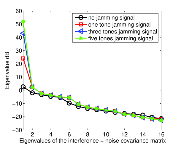
Figure 1: The eigenvalue of the desired-signal-absent covariance matrix.

From the simulation result we can see that the interference energy is mainly located at the principal eigenvalue of the desired-signal-absent covariance matrix. Using this character we can easily know about the existence of the JS. This method is also insensitive to the number of the interferers.

III-B Widely Linear Signal Processing Scheme

In [24] and [25], it has been shown that for BPSK modulation and other non-circular or improper modulation schemes, the performance of linear receivers can be further improved if both the received signal and also its complex conjugate are processed. This is because, for improper signals, the covariance matrix $\boldsymbol{R}_{rr}=E[\boldsymbol{r}\boldsymbol{r}^{H}]$ cannot completely describe the second-order statistics of the received vector and the complementary covariance matrix $\hat{\boldsymbol{R}}=E[\boldsymbol{r}\boldsymbol{r}^{T}]$ needs to be taken into account. The resulting receiver is referred to as a WL receiver.

In order to exploit the second-order information, we perform WL processing that utilizes the received vector $\boldsymbol{r}$ and its complex conjugate $\boldsymbol{r}^{\ast}$ to form an augmented vector. For convenience we introduce the bijective transform $\mathcal{J}\{\cdot\}$

$$\boldsymbol{r}\to\tilde{\boldsymbol{r}}:~{}~{}~{}~{}~{}~{}~{}~{}\tilde{\boldsymbol{r}}=\dfrac{1}{\sqrt{2}}[\boldsymbol{r}^{T},\boldsymbol{r}^{H}]^{T}.$$ (22)

In what follows, all WL based quantities are denoted by an over tilde. An important property of $\mathcal{J}\{\cdot\}$ is that, for a complex vector $\boldsymbol{r}$ and $\boldsymbol{u}$, $\tilde{\boldsymbol{u}}^{H}\tilde{\boldsymbol{r}}=\tilde{\boldsymbol{r}}^{H}\tilde{\boldsymbol{u}}$. Now a widely linear MMSE solution can be directly obtained as

$$\tilde{\boldsymbol{w}}_{k}=\boldsymbol{R}^{-1}_{\tilde{r}\tilde{r}}\tilde{\boldsymbol{p}}_{k},$$ (23)

where

$$\boldsymbol{R}_{\tilde{r}\tilde{r}}=E[\tilde{\boldsymbol{r}}\tilde{\boldsymbol{r}}^{H}]=\dfrac{1}{2}\left[\begin{array}[]{cc}{\boldsymbol{R}}_{rr}&{\hat{\boldsymbol{R}}_{rr}}\\ {\hat{\boldsymbol{R}}_{rr}^{\ast}}&{\boldsymbol{R}}_{rr}^{\ast}\end{array}\right],$$ (24)

$$\tilde{\boldsymbol{p}}_{k}=\mathcal{J}\left\{{\boldsymbol{p}}_{k}\right\}$$ (25)

and the widely linear MMSE estimate of the data symbol is given by

$$\hat{b}_{k}=\mathcal{R}\{\textrm{sgn}(\tilde{\boldsymbol{w}}_{k}\tilde{\boldsymbol{r}})\}.$$ (26)

III-C MC-SIC MMSE Design

As mentioned above, the SIC scheme is a decision-driven detection algorithm which suffers from error propagation and performance degradation, the strategy of the MC-SIC scheme is to find the optimum feedback decision and mitigate the error propagation. The key idea behind the MC-SIC scheme is to exploit the structural properties of the sub-constellation formed by the signals of two consecutive users in an ordered set to gain an improvement in detection performance.

In the following, we detail the MC-SIC algorithm through the procedure for detecting $\hat{\boldsymbol{s}}_{k}[i]$ for user $k$. The detection of the data symbols of the other user can be performed accordingly. The soft estimation of the user $k$’s symbol $u_{k}[i]$ is obtained by using the MMSE detector as

$$u_{k}[i]=\boldsymbol{w}_{k}^{H}\hat{\boldsymbol{r}}_{k}[i],$$ (27)

where the MMSE filter is given by $\boldsymbol{w}_{k}=(\boldsymbol{P}_{k}\boldsymbol{P}_{k}^{H}+\delta^{2}_{n}\boldsymbol{I}_{L})^{-1}\boldsymbol{p}_{k}$, $\boldsymbol{P}_{k}$ denotes the matrix obtained by taking the columns $k,k+1,\cdots,K$ of $\boldsymbol{P}$ and $\hat{\boldsymbol{r}}_{k}[i]$ is the received vector after cancellation of the $k-1$ previously detected symbols.

Based on the estimate of the user $k$’s symbol $u_{k}[i]$, the user $(k+1)$’s symbol can be calculated as

$$u_{k}[i]=\boldsymbol{w}_{k+1}^{H}(\hat{\boldsymbol{r}}_{k}[i]-Q[u_{k[i]}]\boldsymbol{p}_{k}),$$ (28)

where $Q[\cdot]$ is the signal quantization operator used to detect the signals of each user. The detection parameter $a_{f}$ is constructed with the estimated symbols $u_{k}[i]$ and $u_{k+1}[i]$ as

$$a_{f}=\mathcal{R}\{u_{k}[i]\}+\textrm{j}\mathcal{R}\{u_{k+1}[i]\}.$$ (29)

For each user, the reliability of the soft estimate $u_{k}[i]$ is determined by the combined constellation constraint structure which is illustrated in Fig.2.

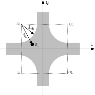
Figure 2: The combined constellation constraint structure. The constellation constraint is invoked as the soft estimate parameter $a_{f}$ is dropped into the shaded area.

The combined constellation constraint structure shown in Fig.2 is for BPSK modulation mode and the combined constellation set is constructed as $\mathcal{A}=\mathcal{\{}a_{1}=-1+\textrm{j},a_{2}=1+\textrm{j},a_{3}=1-\textrm{j},a_{4}=-1-\textrm{j}\}$. The parameter $d_{th}$ is the threshold distance to evaluate the reliability of the current estimated symbol $u_{k}[i]$, which is a predefined parameter. The reliability of the estimated symbol is determined by the Euclidean distance between the detection parameter $a_{f}$ and its nearest combined constellation points, which is given by

$$d_{k}=\mid{a}_{opt}-a_{f}\mid.$$ (30)

The optimum parameter $a_{opt}$ denotes the constellation point which is the nearest to the detection parameter $a_{f}$ and can be expressed as

$$a_{opt}=\textrm{arg min}_{{a_{c}}\in\mathcal{A}}\{\mid a_{c}-a_{f}\mid\}.$$ (31)

There are two possibilities as follows:

1. If $d_{k}\geq{d_{th}}$, then the current soft estimate $u_{k}[i]$ is determined reliable and the estimated symbol of user $k$ is obtained by $\hat{s}_{k}[i]=Q[u_{k}[i]]$. After we get the estimated symbol $\hat{s}_{k}[i]$, we can regenerate user $k$, cancel it from the received vector $\hat{\boldsymbol{r}}_{k}[i]$ and continue the procedure above to estimate user $k+1$.

2. If $d_{k}<d_{th}$, then the current soft estimate $u_{k}[i]$ is determined unreliable and the optimum feedback symbol must be found before cancellation. Since the effect of “closest” interferer is significant in terms of performance degradation while estimating the user $k$’s symbol $\hat{s}_{k}[i]$ [12], we estimate two consecutive user signals $\{s_{k},s_{k+1}\}$ at one time and the candidates for $s_{k}$ and $s_{k+1}$ are selected from $\mathcal{L}=\{\boldsymbol{c}_{1},\boldsymbol{c}_{2},\boldsymbol{c}_{3},\boldsymbol{c}_{4}\}$, where $\boldsymbol{c}_{1}=[-1,+1]$, $\boldsymbol{c}_{2}=[-1,-1]$, $\boldsymbol{c}_{3}=[+1,+1]$, $\boldsymbol{c}_{4}=[+1,-1]$. After the optimum candidate $\boldsymbol{c}_{opt}$ is selected from $\mathcal{L}$, the effects of user $k$ and $k+1$ will be subtracted together before detecting the rest of the users. The selection algorithm is described as follows.

In order to get the optimum candidate $\boldsymbol{c}_{opt}$ for user $k$ and user $k+1$, we construct the estimated symbol vector from three parts: the first part is the previously detected symbols $\hat{s}_{1}[i]$, $\hat{s}_{2}[i]$, $\cdots$, $\hat{s}_{k-1}[i]$, the second part $\boldsymbol{c}_{k}$ is the symbol taken from the candidate constellation point set $\mathcal{L}$, the last part uses the previous decisions and performs the following users $k+2$,$\cdots$,$K$’s detection by the nulling and symbol cancellation which is equivalent to the traditional SIC algorithm. Therefore, we can get the estimated symbol vector

$$\boldsymbol{b}^{m}[i]=[\hat{s}_{1}[i],\cdots,\hat{s}_{k-1}[i],\boldsymbol{c}_{m},b^{m}_{k+2}[i],\cdots,b^{m}_{q}[i],\cdots,b^{m}_{K}[i]],$$ (32)

where $\boldsymbol{c}_{m}\in\mathcal{L}$, $b^{m}_{q}[i]$ is the potential decision that corresponds to the selection of $\boldsymbol{c}_{m}$ in the constellation point set,

$$b^{m}_{q}[i]=Q\left[\boldsymbol{w}^{m}_{k}\hat{\boldsymbol{r}}^{m}_{q}[i]\right].$$ (33)

where $q$ indexes a certain user between $k+2$ to $K$. For each user the same MMSE filter $\boldsymbol{w}_{k}$ is used for all the candidates, which can be calculated in advance and allows the proposed algorithm to have the computational simplicity of the SIC algorithm described by

$$\hat{\boldsymbol{r}}^{m}_{q}[i]=\hat{\boldsymbol{r}}^{m}_{k}[i]-\left[\boldsymbol{p}_{k},\boldsymbol{p}_{k+1}\right]\boldsymbol{c}^{T}_{m}-\sum_{j=k+2}^{q-1}\boldsymbol{p}_{j}b^{m}_{j}[i].$$ (34)

According to the maximum likelihood rule in the selected candidates set, the optimum candidate $\boldsymbol{c}_{opt}$ is given by

$$\boldsymbol{c}_{opt}=\textrm{arg min}_{\boldsymbol{c}_{m}\in\mathcal{L}}{\parallel\boldsymbol{r}[i]-\boldsymbol{P}\boldsymbol{b}^{m}[i]\parallel}^{2},$$ (35)

where the $\boldsymbol{c}_{opt}$ is chosen to replace the unreliable $u_{k}[i]$ and $u_{k+1}[i]$, which will be the optimal feedback symbols for the next user as well as the more reliable estimate for the current two users.

III-D Widely Linear MC-SIC MMSE Algorithm

In this subsection, we will combine widely linear signal processing with the MC-SIC MMSE scheme and obtain the WL-MC-SIC MMSE algorithm.

From the previous subsection, we can compute the widely linear MMSE filter as

$$\hat{\boldsymbol{w}}_{k}=2\left(\begin{array}[]{cc}\left(\boldsymbol{P}_{k}\boldsymbol{P}^{H}_{k}+\sigma^{2}_{n}\boldsymbol{I}_{L}\right)&\left(\boldsymbol{P}_{k}\boldsymbol{P}^{T}_{k}\right)\\ \left(\boldsymbol{P}_{k}\boldsymbol{P}^{T}_{k}\right)^{\ast}&{\left(\boldsymbol{P}_{k}\boldsymbol{P}^{H}_{k}+\sigma^{2}_{n}\boldsymbol{I}_{L}\right)}^{\ast}\end{array}\right)^{-1}\tilde{\boldsymbol{p}}_{k}.$$ (36)

The soft estimate of the user $k$’s symbol $\tilde{u}_{k}[i]$ is obtained by using the WL MMSE detector as

$$\tilde{u}_{k}[i]=\tilde{\boldsymbol{w}}_{k}^{H}\tilde{\boldsymbol{r}}_{k}[i],$$ (37)

where $\tilde{r}_{k}[i]=\mathcal{J}\left\{{\tilde{\boldsymbol{r}}}_{k}[i]\right\}$. The algorithm of the proposed WL-MC-SIC is summarized in Table II.

TABLE II: THE WL MC-SIC ALGORITHM

1:  $\hat{\boldsymbol{w}}_{k}=2\left(\begin{array}[]{cc}\left(\boldsymbol{P}_{k}\boldsymbol{P}^{H}_{k}+\sigma^{2}_{n}\boldsymbol{I}_{L}\right)&\left(\boldsymbol{P}_{k}\boldsymbol{P}^{T}_{k}\right)\\ \left(\boldsymbol{P}_{k}\boldsymbol{P}^{T}_{k}\right)^{\ast}&{\left(\boldsymbol{P}_{k}\boldsymbol{P}^{H}_{k}+\sigma^{2}_{n}\boldsymbol{I}_{L}\right)}^{\ast}\end{array}\right)^{-1}$

2:  $\mathcal{L}=\left\{\boldsymbol{c}_{1},\boldsymbol{c}_{2},\boldsymbol{c}_{3},\boldsymbol{c}_{4}\right\}$

3:   while $k<K$

4:     $\tilde{u}_{k}[i]=\tilde{\boldsymbol{w}}_{k}^{H}\tilde{\boldsymbol{r}}_{k}[i]$

5:     $\tilde{u}_{k+1}[i]=\tilde{\boldsymbol{w}}_{k+1}^{H}(\tilde{\boldsymbol{r}}_{k}[i]-Q\left[\tilde{u}_{k}[i]\right]\tilde{p}_{k})$

6:     $a_{f}=\mathcal{R}\left\{u_{k}[i]\right\}+\textrm{j}\mathcal{R}\left\{u_{k+1}[i]\right\}$

7:     if $d_{k}>d_{th}$

8:       if $k=K-1$

9:         $\boldsymbol{c}_{opt}=\textrm{arg min}_{\boldsymbol{c}_{m}\in\mathcal{L}}{\parallel\boldsymbol{r}[i]-\boldsymbol{P}\boldsymbol{b}^{m}[i]\parallel}^{2}$

10:        $\tilde{s}_{K-1}[i]=\boldsymbol{c}_{opt}(1,1)~{}~{}~{}\tilde{s}_{K}[i]=\boldsymbol{c}_{opt}(1,2)$

11:        $\textrm{loopsym}=1$   % loopsym=1 denotes program execution in

this branch,initial value is 0

12:      else if $k=K-2$

13:             $\tilde{\boldsymbol{r}}^{m}_{K}[i]-[\tilde{\boldsymbol{p}}_{K-2},\tilde{\boldsymbol{p}}_{K-1}]\boldsymbol{c}^{T}_{m}$

14:             $b^{m}_{K}[i]=Q[\tilde{\boldsymbol{w}}^{H}_{K}\tilde{\boldsymbol{r}}^{m}_{K}[i]]$

15:             $\boldsymbol{b}^{m}[i]=\left[\tilde{s}_{1}[i],\cdots,\tilde{s}_{K-3}[i],\boldsymbol{c}_{m},b^{m}_{K}[i]\right]$

16:             $\boldsymbol{c}_{opt}=\textrm{arg min}_{\boldsymbol{c}_{m}\in\mathcal{L}}\parallel\tilde{\boldsymbol{r}}[i]-\tilde{\boldsymbol{P}}\boldsymbol{b}^{m}[i]\parallel^{2}$

17:             $\tilde{{}_{K-2}[i]}=\boldsymbol{c}_{opt}(1,1)~{}~{}\tilde{{}_{K-1}[i]}=\boldsymbol{c}_{opt}(1,2)$

18:             $\tilde{\boldsymbol{r}}_{k}[i]=\tilde{\boldsymbol{r}}_{K-2}[i]-\tilde{s}_{K-2}[i]\tilde{\boldsymbol{p}}_{K-2}-\tilde{s}_{K-1}[i]\tilde{\boldsymbol{p}}_{K-1}$

19:          else

20:            $\tilde{\boldsymbol{r}}_{k+2}^{m}[i]=\tilde{\boldsymbol{r}}_{k}^{m}[i]-\left[\tilde{\boldsymbol{p}}_{k-2},\tilde{\boldsymbol{p}}_{k-1}\right]\boldsymbol{c}^{T}_{m}$

21:            for $j=k+2$ to $K$

22:              $b^{m}_{j}[i]=Q\left[\tilde{\boldsymbol{w}}^{H}_{j}\tilde{\boldsymbol{r}}^{m}_{j}[i]\right]$

23:              $\tilde{\boldsymbol{r}}^{m}_{j+1}=\tilde{\boldsymbol{r}}^{m}_{j}-b^{m}_{j}[i]\tilde{\boldsymbol{p}}_{j}$

24:            end for

25:            $\boldsymbol{c}_{opt}=\textrm{arg min}_{\boldsymbol{c}_{m}\in\mathcal{L}}\parallel\tilde{\boldsymbol{r}}[i]-\tilde{\boldsymbol{P}}\boldsymbol{b}^{m}[i]\parallel^{2}$

26:            $\tilde{s}_{k}[i]=\boldsymbol{c}_{opt}(1,1)~{}~{}~{}\tilde{s}_{k+1}[i]=\boldsymbol{c}_{opt}(1,2)$

27:            $\tilde{\boldsymbol{r}}_{k+2}[i]=\tilde{\boldsymbol{r}}_{k}[i]-\tilde{s}_{k}[i]\tilde{\boldsymbol{p}}_{k}-\tilde{s}_{k+1}[i]\tilde{\boldsymbol{p}}_{k+1}$

28:      end if

29:      $k=k+2$

30:   else

31:     $\tilde{s}_{k}[i]=Q\left[\tilde{u}_{k}[i]\right]$

32:     $\tilde{\boldsymbol{r}}_{k+1}[i]=\tilde{\boldsymbol{r}}_{k}[i]-\tilde{s}_{k}[i]\tilde{\boldsymbol{p}}_{k}$

33:     $k=k+1$

34:   end if

35:  end while

36:  if $\textrm{loopsym}\not=1$

37:     $\tilde{s}_{K}[i]=Q\left[\tilde{\boldsymbol{w}}_{K}^{H}\tilde{\boldsymbol{r}}_{K}[i]\right]$

38:  end if

III-E VSP Scheme and WL-MC-SIC MMSE Detector

In this subsection, the procedure for MAI and JS suppression using the proposed WL-MC-SIC MMSE algorithm along with the VSP scheme is described.

Using the VSP algorithm [44] we can get the desired-signal-absent covariance matrix $\hat{\boldsymbol{R}}_{j+n}$ and perform an eigen-decomposition as in (18). The eigenvalues $\{\hat{\lambda}_{i},~{}i=1,\cdots,L\}$ are obtained and we can set a threshold $d_{\lambda}$ for checking the existence of the JS, which can be calculated as follows

$$d_{\lambda}=\beta\left(\dfrac{1}{D}\sum_{i=1}^{D}\hat{\lambda}_{i+1}\right),$$ (38)

where $\beta$ is a threshold factor and its associated with the power of the JS and the ambient noise. In this paper it is set to $0.2$. $D$ is the number of eigenvalues which are used to estimate the power of the ambient noise and normally it can be set as $D=2$. By comparing the principal eigenvalue $\hat{\lambda}_{1}$ with the threshold $d_{\lambda}$, we can get the information about the existence of the jamming signal. The procedure for MAI and JS suppression using the proposed algorithm is summarized in Table III.

TABLE III: THE ANTI-INTERFERENCE PROCEDURE of VSP and WL-MC-SIC MMSE ALGORITHM

Step1: Calculate the covariance matrix $\hat{\boldsymbol{R}}_{rr}$.

Step2: Calculate the desired-signal-absent covariance matrix $\hat{\boldsymbol{R}}_{j+n}$

using VSP scheme.

Step3: Perform an eigendecomposition on $\hat{\boldsymbol{R}}_{j+n}$

and get the eigenvalues $\{\hat{\lambda}_{i},~{}i=1,\cdots,L\}$.

Step4: Calculate the threshold $d_{\lambda}$.

Step5: Compare the principal eigenvalue $\hat{\lambda}_{1}$ with the threshold $d_{\lambda}$,

if $\hat{\lambda}_{1}>d_{\lambda}$, execute step 6 otherwise execute step 7.

Step6: Perform the JS suppression using the VSP algorithm.

Step7: Perform MAI suppression using the WL-MC-SIC MMSE

and get the estimate of the desired signal.

III-F Complexity Analysis

In this section, we will discuss the computational complexity of the proposed WL-MC-SIC MMSE algorithm compared with other existing algorithms mentioned above.

The $k$-th user is the desired user in this paper, and we should deduct the effects of $k$-1 users before we estimate the $k$-th user. In terms of complex multiplications, the complexity of the proposed algorithm and other existing algorithms as mentioned above is presented in Table IV. We focus only on the complexity of the main successive cancellation procedure since the rest of the operations including the VSP procedure are similar to the algorithms to be compared against.

TABLE IV: THE ANTI-INTERFERENCE PROCEDURE OF VSP AND WL-MC-SIC MMSE ALGORITHM

Algorithm	Required complex multiplications
SIC MMSE	$RN$
MF-SIC MMSE	$RN+MRSN+QRN$
MC-SIC MMSE	$RN+MRS^{2}N+PRN$
WL-SIC MMSE	$2RN$
WL-MF-SIC MMSE	$RN+2MRSN+2QRN$
WL-MC-SIC MMSE	$RN+2MRS^{2}N+2PRN$

The main difference between the SIC MMSE algorithm and the MC-SIC MMSE detector is how to choose the optimum candidates from the constellation points to replace the unreliable estimate. The threshold $d_{th}$ is an important factor on the effect of the algorithm complexity. In Table IV the parameter $R$ denotes the number of times that the optimum candidate will be calculated when the threshold $d_{th}$ is set. The parameter $N$ denotes the length of the MMSE filter. The parameter $S$ denotes the number of candidates in $\mathcal{L}$. The parameter $M$ denotes the unreliable estimate times. The parameters $Q$ and $P$ denote the number of times we need to calculate the third part of the estimated symbol vector $\boldsymbol{b}^{m}[i]$ in the MF-SIC and MC-SIC algorithms respectively and usually $P$ is bigger than $Q$.

The parameter $d_{th}$ has an important influence on the performance and the complexity of algorithms. we should find a trade off between them. In the next section we will simulate the effects of the different $d_{th}$ on the algorithm.

IV SIMULATION RESULTS

In this section, we assess the bit error rate (BER) performance of the proposed WL-MC-SIC MMSE algorithm compared with the existing MAI cancellation algorithms mentioned above. Firstly, the simulations for the selection of parameter threshold $d_{th}$ are made. Secondly, the performance comparisons between the proposed WL-MC-SIC MMSE algorithm and the existing MAI cancellation algorithms are made. Finally, the performance of the MAI and JS suppression of the proposed VSP and WL-MC-SIC MMSE is shown.

In the following simulations, we consider that all the algorithms are used in synchronous DS-CDMA systems employing BPSK modulation and we transmit 10000 information symbols per user in one packet and the results are averaged over independent Monte Carlo runs. The spreading signature used for every user is randomly generated and the sequence length is 16. We assume that all the users have the same power unless otherwise stated.

IV-A Parameter Threshold Setting

As we have discussed above, the threshold $d_{th}$ is crucial to the performance of the proposed algorithm. The threshold $d_{th}$ can be either a constant or a function of the signal power and the noise power, which can also be obtained through simulation in practical applications. In the paper we assess the BER performance of the algorithm under different thresholds to get the optimum threshold. We assume that the number of users is 8 and the SNR varies from -2dB to 12dB. The threshold is set to $d_{th}$ = 0.1, 0.3, 0.5, 0.7, 0.9 and 1.1. The evaluation of the BER performance against the SNR with different values of $d_{th}$ is shown in Fig.3.

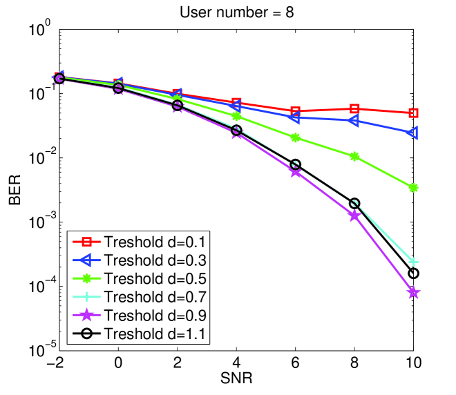
Figure 3: BER performance against SNR(dB) with threshold $d_{th}$ = 0.1, 0.3, 0.5, 0.7, 0.9 and 1.1.

In order to detail the performance difference between the different values of the threshold $d_{th}$, we assess the BER performance of the algorithm at SNR=8dB. The simulation result is shown in Fig.4.

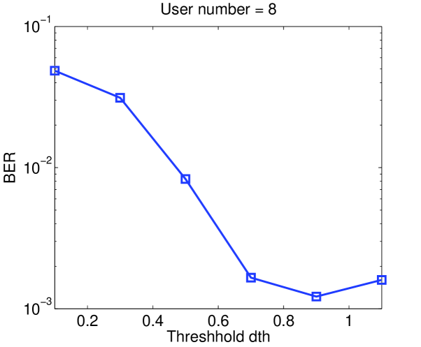
Figure 4: BER performance against threshold with $\textrm{SNR}=8\textrm{dB}$ and the number of user is set to 8.

From the simulation results shown in Fig.3 and Fig.4 we can get the optimum threshold $d_{th}=0.9$. It should be pointed out that the optimum value of $d_{th}$ is relative and it also varies with the different scenarios. The optimum value should be selected under the different scenarios. Unless stated otherwise, in the following scenarios in this paper the threshold $d_{th}$ of the proposed WL-MC-SIC MMSE algorithm is set to $d_{th}=0.9$.

IV-B Performance Comparison

In this subsection, we will compare the BER performance of the proposed WL-MC-SIC MMSE algorithm with the existing MAI cancellation algorithms mentioned above. We use SNR, the capacity in terms of the number of users and algorithm complexity to compare the performance of those algorithms.

Firstly, we evaluate the BER performance against the SNR of the received signal, for the MF-SIC algorithm we choose the optimum threshold $d_{th}=0.3$ which is also obtained through simulation in the same simulation scenario. In the following simulations, we choose this value for the MF-SIC algorithm and the WL-MF-SIC algorithm. The number of users in this scenario is set to 8.

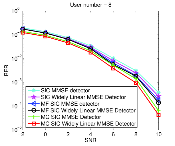
Figure 5: BER performance against SNR with the number of users is set to 8 and SNR varies from -2dB to 10dB.

The simulation result in Fig.5 shows that the BER performance of the WL-MC-SIC MMSE algorithm outperforms other algorithms.

Secondly, we evaluate the BER performance against the number of users. The SNR of this scenario is set to 8dB. The simulation result is illustrated in Fig.6. From the simulation result shown in Fig.6 we can see that with the increase in the number of users, the proposed algorithm has a better performance than the other considered algorithms.

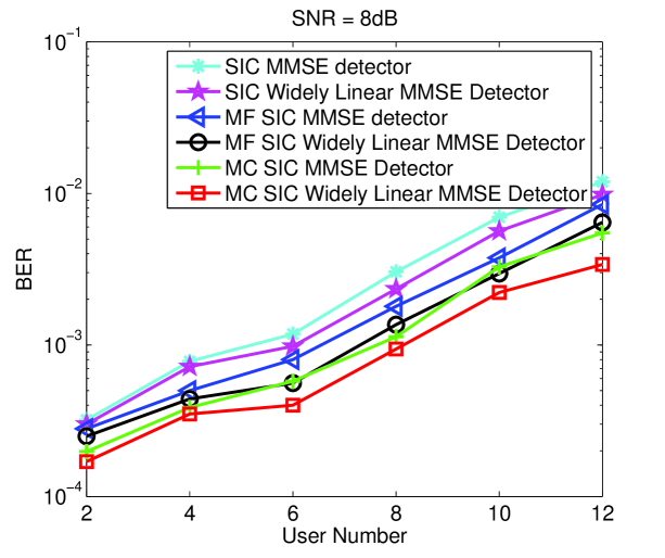
Figure 6: BER performance against the number of users with SNR=8dB and the number of user varies from 2 to 12.

Finally, we will evaluate the algorithm complexity of those algorithms. We have analyzed the algorithm complexity theoretically in Section IV. Here two simulation scenarios will be considered: the first scenario is the algorithm complexity against the length of spreading sequence. The number of users is set to 8 and SNR is set to 8dB. The length of spreading sequence varies from 16 to 128. As mentioned above, we use the number of complex multiplications as the tool to evaluate the complexity of those algorithms. Fig.7(a) shows the simulation result of the first scenario. the second scenario is the algorithm complexity against the number of users and the simulation is shown in Fig.7(b). In the simulation SNR is set to 8dB and the number of users varies from 4 to 12.

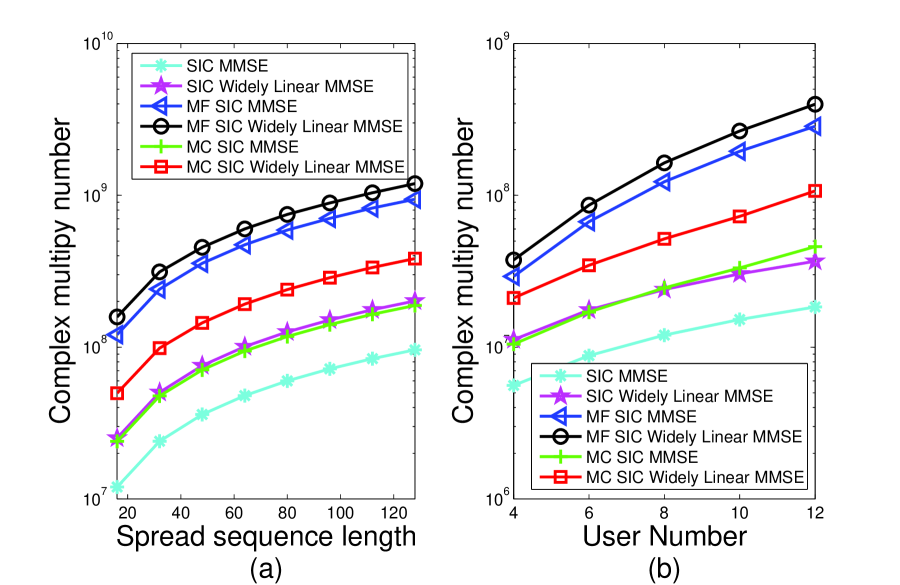
Figure 7: Algorithm complexity simulation, (a) algorithm complexity against the length of spreading sequence, SNR=8dB and the number of users is set to 8, (b)algorithm complexity against the number of users, SNR=8dB and the length of spreading sequence is set to 16.

From the simulation results shown in Fig.7, we find the WL-MC-SIC MMSE algorithm has much less complexity than the WL-MF-SIC MMSE algorithm and the MF-SIC MMSE algorithm. Since the proposed algorithm uses the candidate scheme to alleviate the effect of error propagation in the conventional SIC algorithm, the complexity of the proposed algorithm is inevitably higher than the conventional SIC algorithm.

IV-C Performance of Jamming Suppression

The linear MMSE detection algorithm has a good performance for suppressing the MAI and the JS [28]. In order to get the MMSE detector, we should have the knowledge of the jamming signal, usually which can be obtained through an adaptive strategy [29]. In this subsection we evaluate the performance of the WL-MC-SIC algorithm on joint MAI and JS suppression.

We take the tone interference as the jamming signal and its form is shown in formula (4). From the conclusion we have drawn above we know that the VSP algorithm is insensitive to the number of tone interferers. In the simulation below, we consider a scenario that uses only one tone signal as the JS and the parameter $m=1$. As the VSP algorithm is used to suppress the JS before suppressing the MAI, to be simplicity we only assess the effect of JS suppression of the proposed algorithm, which combines the VSP algorithm with the WL-MC MMSE algorithm together. The other simulation conditions are the same with the simulations above.

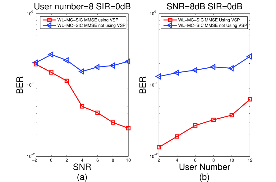
Figure 8: BER performance simulations under the JS scenario and SIR=0dB: (a) BER performance against SNR, the number of users is set to 8, (b) BER performance against the number of user, SNR=8dB.

From the simulation results shown in Fig.8 we can see that using the VSP algorithm to suppress the JS before detecting the desired signals will improve the performance of the SIC detector greatly. The proposed algorithm which combines the VSP method and WL-MC-SIC MMSE algorithm together has a much better performance for MAI and JS suppression than the existing schemes mentioned above.

V Conclusion

A WL-MC-SIC MMSE algorithm for DS-CDMA systems for joint MAI and JS suppression is proposed in this paper. The contributions of our research work are composed of three parts: Firstly, in order to cancel the jamming signal, we present a VSP algorithm which is effective in the JS suppression. This method is able to identify the existence of the jamming signal and is insensitive to the number of the tones. Secondly, we propose the multiple candidates constellation constraints scheme to alleviate the effect of error propagation in the SIC algorithm. In order to deal with the improper characteristic of received signal, widely-linear signal processing is used to make full use of the second-order information of received vector which outperforms linear signal processing. Finally, we propose a WL-MC-SIC MMSE scheme which combines the VSP algorithm with the WL-MC-SIC MMSE algorithm together for joint suppressing MAI and JS. The simulation results show that the proposed algorithm outperforms the existing SIC MMSE algorithms mentioned above and have a good performance for JS suppression.

References

- [1] S. Verdu, “Multiuser Detection’ (Cambridge, Cambridge University Press, 1998, 4th edition)
- [2] P. Patel, J. Holtzman.: ‘Analysis of a simple successive interference cancellation scheme in DS/CDMA system’, IEEE Journal. Select. Areas Commun., 1994, 12, (5), pp.124-134
- [3] D. Divsalar, M. K. Simon, D. Raphaeli.: ‘Improved parallel interference cancellation for CDMA’, IEEE Trans. Commun., 1998, 46, (12), pp.258-268
- [4] P. H. Tan, L. K. Rasmussen.: ‘Constrained maximum-likelihood detection in CDMA’, IEEE Trans. Commun., 2001, 49, (1), pp.142–153
- [5] L. B. Nelson, H. V. Poor.: ‘Iterative multiuser receivers for CDMA channels: An EM approach’, IEEE Trans. Commun., 1996, 44, (12), pp.1700–1710
- [6] H. Elders-Boll, H. D. Schotten, A. Busboom.: ‘Efficient implementation of linear multiuser detectors for asynchronous CDMA systems by linear interference cancellation’, European Trans. Telecommun, 1998, 9, (5), pp.427–437
- [7] W. Zha and S. D. Blostein, “Soft-Decision Multistage Multiuser Interference Cancellation”, IEEE Trans. Vehicular Technology, 2003, 52, (2), pp.380–388.
- [8] K.C. Lai and J. J. Shynk, “Performance evaluation of a generalized linear SIC for DS/CDMA signals”, IEEE Trans. Signal Processing, 2003, 51, (6), pp.1604–1614.
- [9] R. C. de Lamare, R. Sampaio-Neto, “Adaptive MBER decision feedback multiuser receivers in frequency selective fading channels”, IEEE Communications Letters, vol. 7, no. 2, Feb. 2003, pp. 73 - 75.
- [10] P. Li, R. C. de Lamare, R. Fa., “Multiple Feedback Successive Interference Cancellation Detection for Multiuser MIMO Systems”, IEEE Trans. Wireless Communications, 2011, 10, (8), pp.2434–2439.
- [11] R.C. de Lamare, R. Sampaio-Neto, A. Hjorungnes, “Joint iterative interference cancellation and parameter estimation for cdma systems”, IEEE Communications Letters, 11, (12), December 2007, pp. 916 - 918.
- [12] A. Sen Gupta and A. Singer, “Successive Interference Cancellation Using Constellation Structure”, IEEE Trans. Signal Processing, 2007, 55, (12), pp.5716–5730.
- [13] R.C. de Lamare, R. Sampaio-Neto, “Minimum mean-squared error iterative successive parallel arbitrated decision feedback detectors for DS-CDMA systems”, IEEE Transactions on Communications, 56, (5), May 2008, pp. 778-789.
- [14] R. Fa, R. C. de Lamare, “Multi-Branch Successive Interference Cancellation for MIMO Spatial Multiplexing Systems”, IET Communications, 5, (4), pp. 484 - 494, March 2011.
- [15] S. Li, R. C. de Lamare, “Adaptive linear interference suppression based on block conjugate gradient method in frequency domain for DS-UWB systems”, Proc. The Sixth International Symposium on Wireless Communication Systems Conf.,Siena, Italy, September 2009, pp.343-347.
- [16] S. Li and R. C. de Lamare, “Frequency Domain Adaptive Detectors for SC-FDE in Multiuser DS-UWB Systems Based on Structured Channel Estimation and Direct Adaptation”, IET Communications, 4, (13), 2010, pp. 1636-1650.
- [17] R. C. de Lamare and R. Sampaio-Neto, “Blind adaptive code-constrained constant modulus algorithms for CDMA interference suppression in multipath channels”, IEEE Communications Letters, vol. 9, no. 4, pp. 334-336, April 2005.
- [18] R. C. de Lamare and R. Sampaio-Neto, “Blind adaptive MIMO receivers for space-time block-coded DS-CDMA systems in multipath channels using the constant modulus criterion,” IEEE Transactions on Communications, vol. 58, no. 1, January 2010, pp. 21-27.
- [19] L. Wang and R. C. de Lamare, “Constrained adaptive filtering algorithms based on conjugate gradient techniques for beamforming”, IET Signal Processing, vol. 4, no. 6, pp. 686-697, December 2010.
- [20] P. Clarke and R. C. de Lamare, “Low-complexity reduced-rank linear interference suppression based on set-membership joint iterative optimization for DS-CDMA systems”, IEEE Transactions on Vehicular Technology, vol. 60, no. 9, pp. 4324-4337, November 2011.
- [21] S. Li, R. C. de Lamare and R. Fa, “Reduced-rank linear interference suppression for DS-UWB systems based on switched approximations of adaptive basis functions”, IEEE Transactions on Vehicular Technology, vol. 60, no. 2, pp. 485-497, February 2011.
- [22] R. C. de Lamare, R. Sampaio-Neto and M. Haardt, “Blind adaptive constrained constant-modulus reduced-rank interference suppression algorithms based on interpolation and switched decimation”, IEEE Transactions on Signal Processing, vol. 59, no. 2, pp. 681-695, February 2011.
- [23] S. Li and R. C. de Lamare, “Blind reduced-rank adaptive receivers for DS-UWB systems based on joint iterative optimization and the constrained constant modulus criterion”, IEEE Transactions on Vehicular Technology, vol. 60, no. 6, pp. 2505-2518, July 2011.
- [24] B. Picinbono and P. Chevalier, “Widely linear estimation with complex data”, IEEE Trans. Signal Processing, 1995, 43, (8), pp.2030-2033
- [25] P. J. Schreier, L. L. Scharf, “Second-order analysis of improper complex random vectors and processes’, IEEE Trans. Signal Processing, 2003, 51, (3), pp.714-725
- [26] S. Buzzi, M. Lops, A. M. Tulino, “A new family of MMSE multiuser receivers for interference suppression in DS/CDMA systems employing BPSK modulation”, IEEE Trans. Communications, 2001, 49, (1), pp.154-167.
- [27] N. Song, R. C. de Lamare, M. Haardt, and M. Wolf, “Adaptive Widely Linear Reduced-Rank Interference Suppression based on the Multi-Stage Wiener Filter”, IEEE Transactions on Signal Processing, 60, (8), 2012.
- [28] H. V. Poor and X. Wang, ‘Code-Aided Interference Suppression for DS/CDMA Communications-Part I:Interference Suppression Capability’, IEEE Trans. Communications, 1997, 45, (9), pp.1101-1111
- [29] H. V. Poor and X. Wang, “Code-Aided Interference Suppression for DS/CDMA Communications-Part II: Parallel Blind Adaptive Implementations”, IEEE Trans. Communications, 1997, 45, (9), pp.1112-1122
- [30] P. Li and R. C. de Lamare, “Apaptive Decision Feedback Detection with Constellation Constraints for MIMO Systems”, IEEE Trans. Vehicular Technology, 2012, 61, (2), pp.853-859
- [31] L. Milstein, “Interference rejection techniques in spread spectrum communications’, Proc. IEEE Conf., June 1988, pp.657-671
- [32] M. G. Amin, C. Wang, A. R. Lindsey, “Optimum Interference Excision in Spread Spectrum Communications Using Open-Loop Adaptive Filters”, IEEE Trans. Signal Processing, 1999, 61, (7), pp.1966-1096
- [33] E. Panay and Y. Bar-Ness, “Rejection of Multiple Tone Interference in DS Spread-Spectrum Systems Employing Minimum Redundant Transversal Filters”, IEEE Communications Letters, 1997, 1, (5), pp.140-143.
- [34] M. L. Honig and J. S. Goldstein, “Adaptive reduced-rank interference suppression based on the multistage Wiener filter,” IEEE Trans. on Communications, 50, (6), June 2002.
- [35] R. C. de Lamare and R. Sampaio-Neto, “Adaptive reduced-rank MMSE filtering with interpolated FIR filters and adaptive interpolators”, IEEE Signal Processing Letters, vol. 12, no. 3, March, 2005.
- [36] R. C. de Lamare and Raimundo Sampaio-Neto, “Reduced-rank Interference Suppression for DS-CDMA based on Interpolated FIR Filters”, IEEE Communications Letters, vol. 9, no. 3, March 2005.
- [37] R. C. de Lamare and R. Sampaio-Neto, “Adaptive Interference Suppression for DS-CDMA Systems based on Interpolated FIR Filters with Adaptive Interpolators in Multipath Channels”, IEEE Trans. Vehicular Technology, Vol. 56, no. 6, September 2007.
- [38] R. C. de Lamare and R. Sampaio-Neto, “Adaptive Reduced-Rank MMSE Parameter Estimation based on an Adaptive Diversity Combined Decimation and Interpolation Scheme,” Proc. IEEE International Conference on Acoustics, Speech and Signal Processing, April 15-20, 2007, vol. 3, pp. III-1317-III-1320.
- [39] R. C. de Lamare and R. Sampaio-Neto, “Reduced-Rank Adaptive Filtering Based on Joint Iterative Optimization of Adaptive Filters”, IEEE Signal Processing Letters, 14, (12), December 2007.
- [40] R. C. de Lamare, M. Haardt and R. Sampaio-Neto, “Blind Adaptive Constrained Reduced-Rank Parameter Estimation based on Constant Modulus Design for CDMA Interference Suppression,” IEEE Transactions on Signal Processing, 56, (6), June 2008.
- [41] R. C. de Lamare and R. Sampaio-Neto, “Adaptive reduced-rank processing based on joint and iterative interpolation, decimation, and filtering,” IEEE Trans. Signal Processing, 57, (7), July 2009, pp. 2503-2514.
- [42] R. C. de Lamare and R. Sampaio-Neto, “Reduced-Rank Space-Time Adaptive Interference Suppression With Joint Iterative Least Squares Algorithms for Spread-Spectrum Systems,” IEEE Transactions on Vehicular Technology, 59, (3), March 2010, pp.1217-1228.
- [43] R.C. de Lamare and R. Sampaio-Neto, “Adaptive reduced-rank equalization algorithms based on alternating optimization design techniques for MIMO systems,” IEEE Trans. Veh. Technol., vol. 60, no. 6, pp. 2482-2494, July 2011.
- [44] J. Zhuang and A. Manikas, “Interference cancellation beamforming robust to pointing errors”, IET Trans. Signal Processing, 2013, 7, (2), pp.120–127
- [45] H. Stark and Y. Yang, “Vector space projections: a numerical approach to signal and image processing, neural nets, and optics”, ( John Wiley & Sons, New York, NY, USA, 1998)