Vector rogue waves and dark-bright boomeronic solitons in autonomous and nonautonomous settings

Abstract

In this work, we consider the dynamics of vector rogue waves and dark-bright solitons in two-component nonlinear Schrödinger equations with various physically motivated time-dependent nonlinearity coefficients, as well as spatio-temporally dependent potentials. A similarity transformation is utilized to convert the system into the integrable Manakov system and subsequently the vector rogue and dark-bright boomeron-like soliton solutions of the latter are converted back into ones of the original non-autonomous model. Using direct numerical simulations we find that, in most cases, the rogue wave formation is rapidly followed by a modulational instability that leads to the emergence of an expanding soliton train. Scenarios different than this generic phenomenology are also reported.

I Introduction

Over the past few years, models of atomic physics emergent and nonlinear optics kiag with a spatially or temporally dependent nonlinearity have received an increasing amount of attention. More specifically, in the context of atomic Bose-Einstein condensates (BECs), the mean-field Gross-Pitaevskii model has been examined in the presence of temporally BEC or spatially boris varying nonlinearity coefficients. These can be realized also experimentally in this setting (by suitable tuning of the $s$-wave scattering length in space or time) by employing external magnetic mFRM or optical oFRM fields close to Feshbach resonances. On the side of nonlinear optics, nonlinear Schrödinger systems of variable (periodic) dispersion have been explored in connection to dispersion management tur and the corresponding notion of nonlinearity management was also theoretically developed towers ; pelinov and experimentally tested both in the context of solitary waves and in that of prototypical instabilities, such as the modulational instability (MI) psaltis .

On the other hand, one of the prototypical coherent structures that have emerged in recent years as being of relevance to an ever-expanding range of settings consists of rogue waves (also known as freak or extreme waves) k2 . Such waveforms have recently been observed in various experiments carried out in a diverse host of systems, including nonlinear optics opt1 ; opt2 ; opt3 , mode-locked lasers laser , superfluid helium He , hydrodynamics hydro , Faraday surface ripples fsr , parametrically driven capillary waves cap , and plasmas plasma . At the same time, there has been a large volume of theoretical effort aimed at understanding the structural characteristics and dynamical properties of such waves. A number of recent reviews have attempted to summarize different aspects of this effort yan_rev ; solli2 ; onorato . Much of this theoretical understanding has, interestingly, been focused on special solutions of the focusing single-component nonlinear Schrödinger (NLS) equation. These solutions include the rational waveform, first proposed by Peregrine pere , and its generalizations, proposed by Kuznetsov kuz , Ma ma , and Akhmediev akh , as well as Dysthe and Trulsen dt among others.

On the other hand, more recently, there has been a number of studies devoted to rogue waves in multi-component (vector) NLS equations. Generally, such NLS systems have been studied extensively both in the physics of atomic BECs (where they describe different atom species, or mixtures of different spin states of the same atom species emergent ) and in nonlinear optics (where they describe the dynamics of two waves of different frequencies, or two waves of different polarizations in a nonlinear birefringent medium kiag ). Furthermore, two-component NLS equations describe two-wave systems in deep water (crossing sea states), where the increase of the MI growth rate and enlargement of the instability region, was proposed as a possible mechanism for the emergence of extreme wave events onor2 . Rogue waves in such two-component NLS equations have been studied in BEC mixtures konotop ; pors and optics, in connection with the four-wave mixing process fwm , but also in the context of other multi-wave systems –such as the Maxwell-Bloch mb and long-short-wave interaction swlw systems. From a mathematical point of view, exact analytical rogue wave solutions of the two coupled NLS equations were presented for the completely integrable Manakov case manakov in Ref. degasPRL , (see also the recent work ML1 ) while higher-order rogue waves pertaining to this case were recently studied as well horw .

Our efforts in the present paper will be in blending these settings, i.e., in obtaining rogue wave, as well as boomeron-like solutions (that spontaneously reverse their direction –see Ref. degasp and references therein) in two-coupled NLS equations with time-dependent nonlinearities that could be of relevance, as indicated above, both in atomic BECs, as well as –potentially– in nonlinear optics. The technique that we will use relies on performing suitable nonlinear transformations to convert the original non-autonomous model into an integrable one, for which such solutions (rogue waves or boomerons) can be identified –see, e.g., Refs. serkin1 ; jvv1 ; jvv2 ; laks ; yan1 ; lihe1 ; xuhe3 ; hefokas2 ; kannajpa and references therein. However, as noted above, the starting point will be different from these earlier works in that we will use a two-component variant of the NLS equation, featuring both a nonlinearity prefactor dependence on the evolution variable, as well as a parabolic potential (of relevance to BECs) with a frequency dependence on the evolution variable; both linear and nonlinear coupling between the two “species” will be present. Starting from this non-autonomous, yet experimentally realizable variant of the two-component model, suitable transformations allow us to translate the dynamical evolution into the integrable Manakov form. In the latter context, the work of Ref. konotop enables us to examine rogue waves, while the findings of Ref. degasPRL allow us to examine the interaction of the rogue wave with a dark-bright “boomeronic” structure. Furthermore, we examine the robustness of these structures in direct numerical simulations of the original non-autonomous model. Here, generalizing the conclusions of the recent work He2014577 to multiple components, we find that in most cases examined, the background state becomes unstable, giving rise to MI and an expanding array of bright solitons.

Our presentation will be structured as follows. In Sec. II, we present the theoretical formulation of the model, and explore its realizability in current experimental setups. In Sec. III, we turn to numerical results, where we examine the dynamical evolution of the different solutions. Finally, in Sec. IV, we summarize our findings and present some conclusions, as well as future challenges.

II Theoretical Model and Analysis

II.1 The autonomous case

We start by considering a system of two coupled NLS equations, in $(1+1)$ dimensions, with constant nonlinear coefficients; this system is relevant to both atomic BEC physics emergent and nonlinear optics kiag and can be expressed in the following dimensionless form:

$$iE_{1,z}+E_{1,tt}+2\gamma\sum_{l=1}^{2}|E_{l}|^{2}E_{1}+\alpha E_{1}+\sigma E_{2}=0,$$

$$iE_{2,z}+E_{2,tt}+2\gamma\sum_{l=1}^{2}|E_{l}|^{2}E_{2}-\alpha E_{2}+\sigma E_{1}=0,$$ (1)

where $E_{1}$ and $E_{2}$ are the complex electric field envelopes in the context of optics or the wavefunctions of two distinct hyperfine states (e.g., of ⁸⁷Rb for $\gamma<0$, or of ⁷Li for $\gamma>0$) in the context of BECs. Additionally, $z$ and $t$ are the longitudinal and transverse coordinates in the optical setting, while in BECs $z$ plays the role of time as the evolution variable and $t$ is the spatial coordinate. The parameter $\gamma$ represents the nonlinear coefficient while the self-focusing and defocusing case (attractive and repulsive interatomic interactions in BECs) corresponds to $\gamma>0$ and $\gamma<0$, respectively. Finally, $\sigma$ is the normalized linear coupling constant induced by a periodic twist of the birefringence axes in optics (see, e.g., Ref. sciencekanna ), or a Rabi coupling in atomic BECs (see, e.g., Refs. Rabi1 ; Rabi2 ), while $\alpha$ is the phase-velocity mismatch from resonance, i.e., a frequency detuning parameter.

We now apply the following rotational transformation sciencekanna ; Rabi1 ; Rabi2 to Eq. (1) in the case of $\gamma$=$1$ ($\gamma$ will be assumed, hereafter, to be positive, as we will consider the self-focusing and attractive interaction setting),

$$\begin{pmatrix}E_{1}\\ E_{2}\end{pmatrix}=\begin{pmatrix}\cos{\theta}&-\sin{\theta}\\ \sin{\theta}&\cos{\theta}\end{pmatrix}\begin{pmatrix}q_{1}e^{i\Gamma z}\\ q_{2}e^{-i\Gamma z}\end{pmatrix},$$ (2)

where $\Gamma=\sqrt{\alpha^{2}+\sigma^{2}}$ and $\theta=\frac{1}{2}\tan^{-1}(\frac{\sigma}{\alpha})$; this way, the resulting equation becomes the self-focusing integrable Manakov system manakov (see also PRLkanna ):

$$iq_{j,z}+q_{j,tt}+2\sum_{\ell=1}^{2}|q_{\ell}|^{2}q_{j}=0,\quad j=1,2.$$ (3)

An interesting rogue wave solution of the Manakov system (3) has been obtained in Ref. degasPRL using the Darboux transformation:

$$q_{1}(t,z)=\left(\frac{Ga_{1}+Ma_{2}}{F}\right)e^{2i\omega z},$$ (4a)

$$q_{2}(t,z)=\left(\frac{Ga_{2}-Ma_{1}}{F}\right)e^{2i\omega z},$$ (4b)

where $G=(3/2)-8\omega^{2}z^{2}-2a^{2}t^{2}+8i\omega z+|f|^{2}e^{2at}$, $M=4f(at-2i\omega z-\frac{1}{2})e^{at+i\omega z}$, $F=(1/2)+8\omega^{2}z^{2}+2a^{2}t^{2}+|f|^{2}e^{2at}$, $a=\sqrt{a_{1}^{2}+a_{2}^{2}}$, $\omega=a^{2}$, $a_{1}$ and $a_{2}$ are two arbitrary real parameters, and $f$ is a complex parameter. It should be pointed out that the amplitude and intensity of the above rogue wave are different in the two components unlike the rogue waves with the same amplitude in both components konotop . Another striking feature of this solution is that the rogue waves co-exist with dark-bright (boomeron-like) solitons. By using the transformation (2), we construct exact rogue wave solutions of the system (1).

It is interesting to note that when $a_{2}=0$ and $f=0$, the rogue wave appears in the $q_{1}$ component, whereas the $q_{2}$ component of the rogue wave vanishes. But in the presence of self- and cross-coupling parameters even for vanishing $a_{2}$ and $f$, the rogue waves still appear in both the components $E_{1}$ and $E_{2}$ without oscillation of the background [see Figs. 1-1]. On the contrary and for non-vanishing values of $a_{1}$ and $a_{2}$ with $f=0$, rogue waves appear over an oscillating background [see Figs. 1-1]. In fact, it can be shown analytically that the oscillations are due to the term: $2a_{1}a_{2}\sin\theta\cos\theta e^{2\Gamma z}$ which vanishes when $a_{1}$ (or $a_{2}$) becomes zero. Furthermore, the linear coupling parameter can be advantageously used for controlling the formation of rogue waves. On the other hand, the existence of the boomeronic type dark-bright (DB) solitons together with rogue waves in the Manakov system requires non-zero values of $a_{1}$, $a_{2}$, and $f$ degasPRL . Remarkably, the system (1) supports a slowly moving boomeronic DB soliton co-existing with rogue waves even for $a_{1}=0$ and $a_{2},f\neq 0$. The latter scenario is depicted in Fig. 2. It should be noted that as $a_{1}$, $a_{2}$, and $f$ vary, we observe that if the amplitude of the DB soliton is increased (by tuning appropriately these parameters), then the amplitude of the rogue wave will be decreased and vice versa. Having discussed the constant (coupling) coefficient case, we now proceed with the case of modulated (in the evolution variable) system parameters.

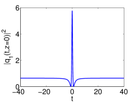
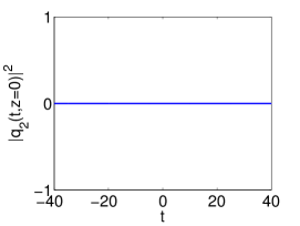
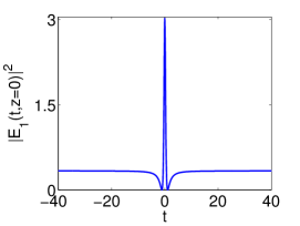
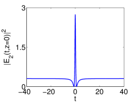
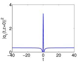
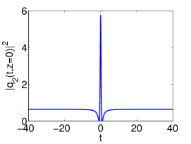
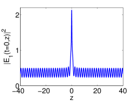
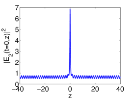
Figure 1: (Color online) Exact rogue waves solutions in the absence (first and third rows) and presence (second and fourth rows) of self- and cross- coupling parameters. Panels (a) and (b) and (c) and (d) correspond to values of the parameters of $a_{1}=0.8$, $a_{2}=0$, $f=0$, $\sigma=1$, and $\alpha=0.05$, whereas (e) and (f) and (g) and (h) correspond to values of the parameters of $a_{1}=0.6$, $a_{2}=0.8$, $f=0$, $\sigma=0.5$, and $\alpha=1.8$.

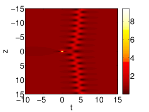
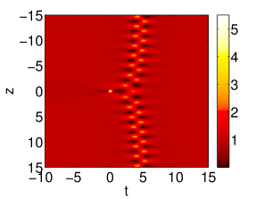
Figure 2: (Color online) Contour plots of the density profiles $|E_{1}(t,z)|^{2}$ (left panel) and $|E_{2}(t,z)|^{2}$ (right panel) over space-time corresponding to the exact solutions in the form of boomeronic DB solitons in the presence of self- and cross-coupling parameters with $a_{1}=0$, $a_{2}=1.3$, $f=0.15$, $\sigma=0.8$, and $\alpha=0.1$.

II.2 Nonlinearity management of rogue waves

We now turn our focus to an inhomogeneous generalization of the NLS system of Eqs. (1) with variable nonlinearity coefficient; this model is expressed in dimensionless form as follows:

$$iE_{1,z}+E_{1,tt}+2\gamma(z)\sum_{l=1}^{2}|E_{l}|^{2}E_{1}+\left[\upsilon(t,z)+\alpha\right]E_{1}+\sigma E_{2}=0,$$

$$iE_{2,z}+E_{2,tt}+2\gamma(z)\sum_{l=1}^{2}|E_{l}|^{2}E_{2}-\left[\alpha-\upsilon(t,z)\right]E_{2}+\sigma E_{1}=0.$$ (5)

Our motivation, as indicated also above, stems from the possibility to modulate $\gamma$ in the evolution variable by means of either Feshbach resonances in BEC mFRM ; oFRM or by means of layered optical media in nonlinear optics psaltis . Additionally, Eq. (5) features an external potential which is given by $\upsilon(t,z)$. This potential will be assumed to be parabolic in the transverse variable $t$ (accounting for a linear parabolic refractive index profile in optics, or a harmonic trapping potential in BECs), while it will also be assumed to be modulated in the evolution variable $z$, i.e., $\upsilon(t,z)=F(z)t^{2}/2$. This way, the parabolic refractive index (in optics) or the parabolic trap (in BECs) is also modulated in the propagation direction (in optics) or in time (in BECs). Examples of such modulations have again arisen in recent experimental efforts in optics szameit , while they have been widely used in the physics of BECs emergent .

Now, we introduce the following rotational transformation to Eq. (5):

$$\begin{pmatrix}E_{1}\\ E_{2}\end{pmatrix}=\begin{pmatrix}\cos{\theta}&-\sin{\theta}\\ \sin{\theta}&\cos{\theta}\end{pmatrix}\begin{pmatrix}\phi_{1}e^{i\Gamma z}\\ \phi_{2}e^{-i\Gamma z}\end{pmatrix},$$

where $\Gamma$ = $\sqrt{\sigma^{2}+\alpha^{2}}$ and $\theta=\frac{1}{2}\tan^{-1}(\sigma/\alpha)$. The resulting equation can be rewritten in the following manner:

$$i\phi_{j,z}+\phi_{j,tt}+2\gamma(z)\sum_{\ell=1}^{2}|\phi_{\ell}|^{2}\phi_{j}+\upsilon(t,z)\phi_{j}=0,\quad j=1,2.$$ (6)

We introduce the similarity transformation

$$\phi_{j}(t,z)=\zeta_{1}\sqrt{\gamma(z)}~{}e^{i\varphi(t,z)}q_{j}[T(t,z),Z(z)],\quad j=1,2,$$ (7a)

together with a quadratic ansatz for the phase:

$$\varphi=-\frac{1}{4}\left[\frac{d}{dz}(\ln\gamma)\right]t^{2}+\zeta_{2}\zeta_{1}^{2}\left(\gamma t-\zeta_{2}\zeta_{1}^{2}\int\gamma^{2}dz\right),$$ (7b)

and the coordinate transformation

$$T=\zeta_{1}\left(\gamma t-2\zeta_{2}\zeta_{1}^{2}\int\gamma^{2}dz\right),$$ (7c)

$$Z=\zeta_{1}^{2}\int\gamma^{2}dz,$$ (7d)

to obtain a standard self-focusing integrable Manakov system:

$$iq_{j,Z}+q_{j,TT}+2\sum_{\ell=1}^{2}|q_{\ell}|^{2}q_{j}=0,\quad j=1,2,$$ (8a)

along with the following integrability condition:

$$F(z)=-\frac{1}{2\gamma}\frac{d^{2}\gamma}{dz^{2}}+\frac{1}{\gamma^{2}}\left(\frac{d\gamma}{dz}\right)^{2}.$$ (8b)

Now, we can reconstruct the exact form of the rogue wave solution of Eq. (5):

$$E_{1}(t,z)=\rho\left(\cos\theta e^{i(\Gamma z+\varphi)}(\bar{G}a_{1}+\bar{M}a_{2})-\sin\theta e^{i(-\Gamma z+\varphi)}(\bar{G}a_{2}-\bar{M}a_{1})\right),$$ (9a)

$$E_{2}(t,z)=\rho\left(\sin\theta e^{i(\Gamma z+\varphi)}(\bar{G}a_{1}+\bar{M}a_{2})+\cos\theta e^{i(-\Gamma z+\varphi)}(\bar{G}a_{2}-\bar{M}a_{1})\right),$$ (9b)

where $\rho=\frac{\zeta_{1}\sqrt{\gamma}}{\bar{F}}e^{2i\omega Z}$, $\bar{G}=(3/2)-8\omega^{2}Z^{2}-2a^{2}T^{2}+8i\omega Z+|f|^{2}e^{2aT}$, $\bar{M}=4f(aT-2i\omega Z-\frac{1}{2})e^{aT+i\omega Z}$, $\bar{F}=(1/2)+8\omega^{2}Z^{2}+2a^{2}T^{2}+|f|^{2}e^{2aT}$ and the coordinates $T$ and $Z$ are given by Eqs. (7c)-(7d).

II.2.1 Periodically modulated nonlinearity coefficient

For purposes of illustration, we now give some specific, yet realistic examples of the nonlinear coefficient and linear potential prefactor variations. First we choose a periodic form of the nonlinearity coefficient, namely,

$$\gamma(z)=1+\varepsilon\cos(z),$$ (10a)

where $$\varepsilon$$ is a real arbitrary parameter. Periodic variations of the nonlinearity coefficient are commonly considered both in BECs BEC ; pelinov and in layered optical media towers ; psaltis . The accompanying evolutionary modulation of the trap frequency reads:

$$F(z)=\frac{\varepsilon[\cos(z)+\varepsilon\cos^{2}(z)+2\varepsilon\sin^{2}(z)]}{2[1+\varepsilon\cos(z)]^{2}}.$$ (10b)

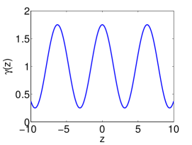
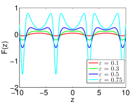
Figure 3: (Color online) Typical form of variable nonlinearity coefficient $\gamma(z)$ for $\varepsilon=0.75$ and trap frequency $F(z)$ for various values of $\varepsilon$.

Figure 3 depicts the profiles of the variable nonlinearity coefficient $\gamma(z)$ and trap frequency $F(z)$ given by Eqs. (10a) and (10b), respectively. In this case, in the absence of cross- and self- coupling parameters $\sigma$ and $\alpha$, the Peregrine bump is not deformed from the original structure, while the dark-bright soliton’s central position is varied with respect to the propagation coordinate $z$, as well as the amplitude increases in both $\phi_{1}$ and $\phi_{2}$ components. In the presence of coupling parameters, the dark-bright solitons may exhibit oscillations (creeping soliton), e.g., for a smaller value of $\sigma$ and larger value of $\alpha$, whereas for larger values of $\sigma$ and smaller $\alpha$’s, the boomeronic behavior is encountered.

II.2.2 Kink-like nonlinearity coefficient

We also chose to examine another form of variable nonlinearity coefficient, enabling the transition between two distinct (constant) values of $\gamma$, namely,

$$\gamma(z)=2+\tanh(\varepsilon z),$$ (11a)

where $$\varepsilon$$ is, again, a real arbitrary parameter, while the associated form of trap frequency is:

$$F(z)=\frac{\varepsilon^{2}\mbox{sech}^{2}(\varepsilon z)[1+2~{}\tanh(\varepsilon z)]}{[2+\tanh(\varepsilon z)]^{2}}.$$ (11b)

In this case, we envision a nonlinearity that is rapidly varied from one value to another as is often done, e.g., in atomic condensates to explore the response of the condensate to such variations hulet .

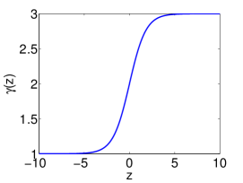
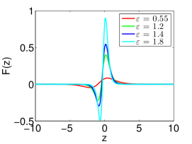
Figure 4: (Color online) Profiles of nonlinearity $\gamma(z)$ (for $\varepsilon=0.55$) and trap frequency $F(z)$ given by Eqs. (11a) and (11b), respectively.

The graphical form of the nonlinearity coefficient and of the trap frequency as a function of the evolution variable are shown in Fig. 4. The modulation of the confining potential $F(z)$ is an asymmetric localized pulse of finite duration; see the right panel of the figure.

In observing the two components in this case, we see that the rogue waves are located on a modified (kink-like, as the kink-like variation in the nonlinearity and linear potential sets in) background. Furthermore, given the functional form of $\gamma(z)$=2+$\tanh(\varepsilon z)$, the soliton expansion begins at the initial value of $z$. On the contrary, when $z>0$, the DB soliton is compressed into a higher amplitude and narrower one.

Having provided the above analytical descriptions for the two different (physically relevant) cases of $\gamma(z)$ [and $F(z)$], we now turn to a series of numerical results. These will help elucidate the states considered (vector rogue waves and rogue-boomeron solution complexes) and their dynamical robustness and observability.

III Computational Analysis

III.1 Numerical method

In what follows, numerical results are presented for the direct numerical integration of Eqs. (5) over the evolution variable by discretizing the $t$ variable, i.e., converting the system of partial differential equations (PDEs) into a system of ordinary differential equations (ODEs). In the same spirit as in Ref. He2014577 , we explore the robustness of the exact solutions describing both Peregrine and interacting Peregrine-DB solitons of Eqs. (5) [by tuning both the coupling parameters and those involved in Eqs. (9a) and (9b) appropriately], under the presence of numerically induced perturbations (caused by round-off and truncation errors). Briefly, the numerical method can be summarized as follows.

At first, the second-order spatial derivatives with respect to $t$ arising in Eqs. (5) are replaced by fourth-order central difference formulas on a uniform spatial grid (with half-width $L$) consisting of $N$ points and lattice spacing $\Delta{t}$ with $t_{j}=-L+2jL/(N+1)$, respectively. In all numerical experiments presented herein, the grid’s half-width and resolution are chosen to be $L=500$ and $\Delta{t}=0.05$ (except for the case of Fig. 5 where $L=300$), respectively, and both are kept fixed. It should be noted that although the fourth-order central difference formulas for the spatial derivatives with respect to $t$ require a wide five-point stencil, one point away both from the left and right boundaries, we use instead second-order central difference formulas. As far as boundary conditions are concerned, no-flux ones are applied, namely, $E_{j,t}(t,z)|_{t=-L}=E_{j,t}(t,z)|_{t=L}=0$, with $j=1,2$. The latter are coupled into the internal discretization scheme using second-order forward and backward difference formulas, respectively.

The temporal integration of the underlying system of ODEs is performed using the Dormand and Prince method (DOP853) with an automatic time-step adaptation procedure (cf. the Appendix in Ref. Hairer ). Furthermore, our numerical results are corroborated using the standard fourth-order Runge-Kutta method (RK4) with fixed time step (typically $\Delta{z}=10^{-5}$ or $10^{-6})$, although numerical results are presented using only the DOP853 method throughout this section; we have nevertheless confirmed that the results of RK4 are essentially identical. We initialize the dynamics using the exact vector rogue wave solutions given by Eqs. (9a) and (9b) adjusted to the particular cases presented below (see also Table 1 for details about parameter values), and consider both periodic and kink-like modulated nonlinearities given by Eqs. (10a) and (11a), respectively. Finally, our numerical integrator is initialized (in all cases studied) at $z_{i}=-3$, since the rogue waves in the vector system appear around $z=0$ and this way, we keep track of the dynamical evolution of the solutions shortly before high amplitude coherent structures arise.

III.2 Numerical results

Next, we present results of our numerical simulations for the vector rogue wave solutions of Eqs. (5). Specifically, Figs. 5 and 6 correspond to rogue wave solutions using the periodic nonlinearity (10a), whereas Figs. 7 and 8 correspond to rogue wave solutions using the kink-like nonlinearity (11a). The corresponding final times of the duration of the simulations reported in this section are $z_{f}=18,18,6,12$, respectively, in these figures. In addition, the left and right panels correspond to density profiles of the fields $E_{1}$ and $E_{2}$, respectively. Note that panels (a)-(d) demonstrate the density profiles $|E_{j}(t,z)|^{2}$ ($j=1,2$) obtained numerically (blue line), in contrast to the corresponding ones from the exact solutions (dash-dotted red line). The first row presents the square modulus of the profile of the two fields as a function of the spatial variable $t$ (at the time-frame of maximum rogue wave density), while the second one the evolution over $z$ (at the position of maximum rogue wave density). Finally, panels (e)-(h) depict space-time contour plots of the density profiles of each component obtained numerically, and, in particular, panels (g) and (h) of the last row illustrate the local densities of each component near the instance of the formation of the rogue wave (near that instance, the reversal of direction of the DB boomeronic structure is clearly evident).

Table 1: Summary of particular cases studied together with parameter values chosen.

Figure	Nonlinearity	$a_{1}$	$a_{2}$	$\zeta_{1}$	$\zeta_{2}$	$f$	$\varepsilon$	$\sigma$	$\alpha$
5	Periodic	$0.8$	$0.2$	$1$	$1$	$0$	$0.3$	$1$	$0$
6		$0$	$0.3$	$1.5$	$0$	$0.15$	$0.3$	$1.5$	$3$
7	Kink-like	$0.6$	$0.8$	$0.6$	$0$	$0$	$1.3$	$0.55$	$2$
8		$0$	$0.5$	$1$	$0$	$0.15$	$0.8$	$1$	$0.2$

Let us now briefly summarize the numerical results presented in this section. It can be discerned immediately in all the cases studied that vector rogue waves can be formed (see Figs. 5 and 7); additionally, waveforms involving the co-existence of rogue waves and DB boomeronic solitons can also naturally arise from suitable initial data (see Figs. 6 and 8) in the transformed system. These solutions directly emerge from the corresponding rogue and rogue-DB solutions of the regular Manakov problem konotop ; degasPRL , yet they bear additional features. In particular, Figs. 5 and 6 contain a periodic modulation of the profile in $z$ (for a given $t$), while Figs. 7 and 8 feature a “jump” in the field value as the nonlinearity “step” is traversed.

However, there is an additional important feature arising past the formation of these high amplitude solitons. In particular, the numerically obtained solutions start to differ from their exact counterparts (except for the case of Fig. 6 where both exact and numerical solutions agree within the reported time of the particular simulation). Following the reasoning of the work konotop (see also He2014577 ), it can be argued that, indeed, any destruction of the exact solutions originating from numerical (e.g., round-off and truncation) errors, which in turn, contribute to perturbations of the solutions, stems from the emergence of the modulational instability (MI) kiag . For instance, in Figs. 5 and 5 the numerical solutions, even beyond the time of occurrence of the high amplitude solitons, accurately capture their exact counterparts, although at later times deviations arise and eventually lead to progressively increasing solitary wave patterns. In fact, the same picture holds in Figs. 7 and 7, however in this case the numerical errors have been amplified earlier and past the formation of the vector rogue waves, the MI leads to the formation of a soliton train. It perhaps comes as no surprise that the instability’s origin is exactly at the very location of the large amplitude waves (such as the rogue waves), as it is in these spots that the rapid growth of the field leads to the most significant amplification of the approximation errors. It is for that reason that the emerging soliton train arises in the form of a “sprinkler” (see, e.g., also kody for a similar example).

Finally, in Figs. 6 and 8 the interaction between rogue waves and solitons with boomeronic behavior is presented while $f$, $a_{2}\neq 0$, and $a_{1}=0$ (see, for details, Table 1). According to degasPRL , this is the case for the integrable Manakov system where all the parameters $a_{1}$, $a_{2}$, and $f$ are strictly non-vanishing, and we expect the emergence of the combined rogue wave-boomeronic DB wave structure. In Fig. 8, shortly after the occurrence of the boomeron-like soliton, the perturbations eventually lead again to MI. Interestingly, in contrast, this is not the case in Fig. 6 where the numerical solutions faithfully reproduce the corresponding exact ones within the time window of the particular simulation. Indeed, the relatively small amplitude of the field $E_{1}$ compared to its counterpart $E_{2}$, possibly inhibits any substantial amplification of numerically induced perturbations for the propagation intervals monitored herein. Nevertheless, and despite the avoidance of the manifestation of the instability in this example, in the vast majority of cases that we have examined (beyond the typical ones reported here), the instability has been observed, especially for sizable amplitudes of the background field, reflecting its significance in terms of the observable behavior in the system (e.g., when monitored in numerical or physical experiments).

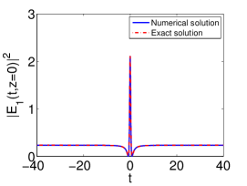
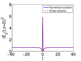
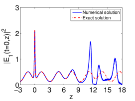
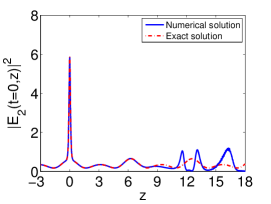
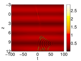
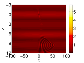
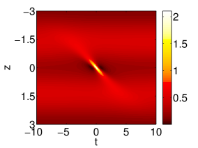
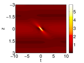
Figure 5: (Color online) Dynamics of rogue waves with a periodically modulated nonlinearity $\gamma(z)$ given by Eq. (10a) and the corresponding trap frequency of Eq. (10b). Left and right panels correspond to density profiles of the numerically obtained fields $E_{1}$ and $E_{2}$, respectively. The top panels (a-b) show the spatial distribution of the intensities $|E_{j}|^{2}$ ($j=1,2$) evaluated at $z=0$, whereas the second row panels (c-d) show their corresponding temporal evolution at $t=0$. The third row panels (e-f) show contour plots of the density profiles of the corresponding rogue waves and the fourth row ones (g-h) zoom-ins of (e-f).

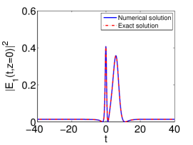
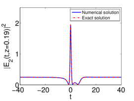
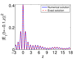
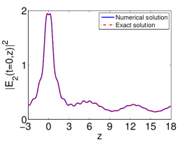
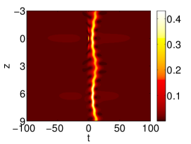
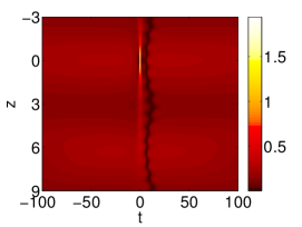
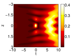
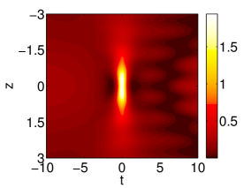
Figure 6: (Color online) Dynamics of co-existing Peregrine and DB boomeronic solitons with a periodically modulated nonlinearity (10a). Left and right panels correspond to density profiles of the numerically obtained fields $E_{1}$ and $E_{2}$, respectively. The top row panels (a-b) show the spatial distribution of the intensities $|E_{1}|^{2}$ at $z=0$ (left) and $|E_{2}|^{2}$ at $z=0.19$ (right), whereas the second row panels (c-d) show their corresponding temporal evolution at $t=-0.1$ and $t=0$, respectively. Again, the panels (e-h) show contour plots of the density profiles of the corresponding waves.

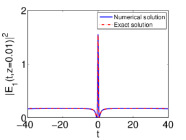
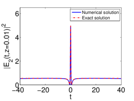
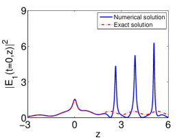
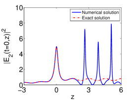
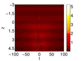
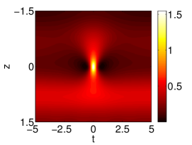
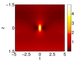
Figure 7: (Color online) Same as Fig. 5 but for the kink-like modulated nonlinearity given by Eq. (11a) and the trap frequency of Eq. (11b). Left and right panels correspond to density profiles of the numerically obtained fields $E_{1}$ and $E_{2}$, respectively. The top row panels (a-b) show the spatial distribution of the intensities $|E_{j}|^{2}$ ($j=1,2$) evaluated at $z=0.01$, whereas the second row panels (c-d) show their corresponding temporal evolution at $t=0$. The panels (e-h) show contour plots of the density profiles of the corresponding rogue waves.

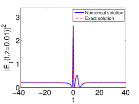
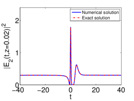
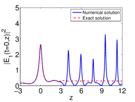
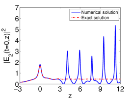
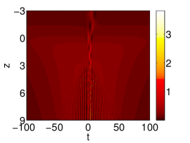
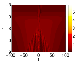
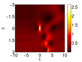
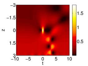
Figure 8: (Color online) Same as Fig. 6 but for the kink-like modulated nonlinearity given by Eq. (11a). Left and right panels correspond to density profiles of the numerically obtained fields $E_{1}$ and $E_{2}$, respectively. The top row panels (a-b) show the spatial distribution of the intensities $|E_{1}|^{2}$ at $z=0.01$ (left) and $|E_{2}|^{2}$ at $z=0.02$ (right), whereas the second row panels (c-d) show their corresponding temporal evolution at $t=0$. The panels (e-h) show contour plots of the density profiles of the corresponding rogue waves.

IV Conclusions and Future Challenges

In the present work, we have revisited the theme of settings presenting modulations in the evolution variable by combining a few relevant, tractable features therein. On the one hand, our starting point was a vector nonlinear Schrödinger system of relevance to both atomic BECs and nonlinear optics, by virtue of specialized yet experimentally tractable settings that were proposed. These featured periodic or hyperbolic dependencies on the evolution variable of the nonlinearity coefficient and the parabolic potential prefactor. We used suitable transformations to convert the non-autonomous version of these multi-component systems into their autonomous siblings. Finally, we explored an intriguing set of recently proposed waveforms in such systems, namely the rogue wave in the form of a Peregrine multi-component soliton, as well as a combination of the rogue wave with a dark-bright solitonic boomeron. Our direct numerical simulations indicated that, indeed, such waveforms were supported and can be observed in the modulated, non-autonomous systems, yet their evolution as perturbed by minimal errors (including round-off and local truncation errors) leads typically to the prominent manifestation of the modulational instability, which, in turn, led to the generation of solitonic trains “emanating” from the location of the principal, large amplitude waves.

There are numerous future directions that can be envisioned as the continuation of the present work. On the one hand, while the current setting refers to “pseudo-spinor” systems (i.e., bearing two components), genuine spinor BECs with more than two components are an intense object of study in the realm of BECs ueda . On the other hand, one can envision generalizing the present considerations (and transformations) to other classes of equations, including to two-dimensional generalizations and non-autonomous variants of models, such as the Kadomtsev-Petviashvili or the Davey-Stewartson equation among others infeld . Such systems are currently under active consideration and will be reported in future publications.

Acknowledgments. E.G.C. gratefully acknowledges financial support from the FP7 People IRSES-606096: “Topological Solitons, from Field Theory to Cosmos”. He also thanks Hans Johnston (UMass) for providing computing facilities. P.G.K. also acknowledges support from the National Science Foundation under grants CMMI-1000337, DMS-1312856, from the Binational Science Foundation under grant 2010239, from FP7-People under grant IRSES-606096 and from the US-AFOSR under grant FA9550-12-10332. The work of D.J.F. was partially supported by the Special Account for Research Grants of the University of Athens. Finally, the work of T.K. and R.B.M. was partially supported by the DST, India under Grant No.SR/S2/HEP-19/2009.

References

- (1) P. G. Kevrekidis, D. J. Frantzeskakis, and R. Carretero-González, Emergent Nonlinear Phenomena in Bose-Einstein Condensates: Theory and Experiment (Springer-Verlag, Heidelberg, 2008); R. Carretero-González, D. J. Frantzeskakis, and P. G. Kevrekidis, Nonlinearity 21, R139 (2008).
- (2) Yu. S. Kivshar and G. P. Agrawal, Optical Solitons: From Fibers to Photonic Crystals (Academic Press, New York, 2003).
- (3) H. Saito and M. Ueda, Phys. Rev. Lett. 90, 040403 (2003). P. G. Kevrekidis, G. Theocharis, D. J. Frantzeskakis, and B. A. Malomed, ibid. 90, 230401 (2003); F. Kh. Abdullaev, A. M. Kamchatnov, V. V. Konotop, and V. A. Brazhnyi ibid. 90, 230402 (2003); F. Kh. Abdullaev, J. G. Caputo, R. A. Kraenkel and B. A. Malomed, Phys. Rev. A 67, 013605 (2003).
- (4) Y. V. Kartashov, B. A. Malomed, and L. Torner, Rev. Mod. Phys. 83, 405 (2011).
- (5) S. Inouye, M. R. Andrews, J. Stenger, H. J. Miesner, D. M. Stamper-Kurn, and W. Ketterle, Nature (London) 392, 151 (1998); J. Stenger, S. Inouye, M. R. Andrews, H.-J. Miesner, D. M. Stamper-Kurn, and W. Ketterle, Phys. Rev. Lett. 82, 2422 (1999); J. L. Roberts, N. R. Claussen, J. P. Burke, Jr., C. H. Greene, E. A. Cornell, and C. E. Wieman, ibid. 81, 5109 (1998); S. L. Cornish, N. R. Claussen, J. L. Roberts, E. A. Cornell, and C. E. Wieman, ibid. 85, 1795 (2000).
- (6) F. K. Fatemi, K. M. Jones, and P. D. Lett, Phys. Rev. Lett. 85, 4462 (2000); M. Theis, G. Thalhammer, K. Winkler, M. Hellwig, G. Ruff, R. Grimm, and J. H. Denschlag, ibid. 93, 123001 (2004).
- (7) S. K. Turitsyn, B. G. Bale, and M. P. Fedoruk, Phys. Rep. 521, 135 (2012).
- (8) I. Towers and B. A. Malomed, J. Opt. Soc. Am. B 19, 537 (2002).
- (9) D. E. Pelinovsky, P. G. Kevrekidis, and D. J. Frantzeskakis, Phys. Rev. Lett. 91, 240201 (2003); D. E. Pelinovsky, P. G. Kevrekidis, D. J. Frantzeskakis and V. Zharnitsky, Phys. Rev. E 70, 047604 (2004).
- (10) M. Centurion, M. A. Porter, P.G. Kevrekidis and D. Psaltis, Phys. Rev. Lett. 97, 033903 (2006); M. Centurion, M. A. Porter, Y. Pu, P. G. Kevrekidis, D. J. Frantzeskakis, D. Psaltis, ibid. 97, 234101 (2006); Phys. Rev. A 75, 063804 (2007).
- (11) C. Kharif, E. Pelinovsky, and A. Slunyaev, Rogue Waves in the Ocean (Springer, New York, 2009).
- (12) D. R. Solli, C. Ropers, P. Koonath, and B. Jalali, Nature (London) 450, 1054 (2007).
- (13) B. Kibler et al., Nat. Phys. 6, 790 (2010).
- (14) B. Kibler et al., Sci. Rep. 2, 463 (2012).
- (15) C. Lecaplain, Ph. Grelu, J. M. Soto-Crespo, and N. Akhmediev, Phys. Rev. Lett. 108, 233901 (2012).
- (16) A. N. Ganshin, V. B. Efimov, G. V. Kolmakov, L. P. Mezhov-Deglin, and P. V. E. McClintock, Phys. Rev. Lett. 101, 065303 (2008).
- (17) A. Chabchoub, N. P. Hoffmann, and N. Akhmediev, Phys. Rev. Lett. 106, 204502 (2011); A. Chabchoub, N. Hoffmann, M. Onorato, and N. Akhmediev, Phys. Rev. X 2, 011015 (2012); A. Chabchoub and M. Fink, Phys. Rev. Lett. 112, 124101 (2014).
- (18) H. Xia, T. Maimbourg, H. Punzmann, and M. Shats, Phys. Rev. Lett. 109, 114502 (2012).
- (19) M. Shats, H. Punzmann, and H. Xia, Phys. Rev. Lett. 104, 104503 (2010).
- (20) H. Bailung, S. K. Sharma, and Y. Nakamura, Phys. Rev. Lett. 107, 255005 (2011).
- (21) Z. Yan, J. Phys. Conf. Ser. 400, 012084 (2012).
- (22) P. T. S. DeVore, D. R. Solli, D. Borlaug, C. Ropers, and B. Jalali, J. Opt. 15, 064001 (2013).
- (23) M. Onorato, S. Residori, U. Bortolozzo, A. Montinad, and F. T. Arecchi, Phys. Rep. 528, 47 (2013).
- (24) D. H. Peregrine, J. Aust. Math. Soc. B 25, 16 (1983).
- (25) E. A. Kuznetsov, Sov. Phys.-Dokl. 22, 507 (1977).
- (26) Ya. C. Ma, Stud. Appl. Math. 60, 43 (1979).
- (27) N. N. Akhmediev, V. M. Eleonskii, and N. E. Kulagin, Theor. Math. Phys. 72, 809 (1987).
- (28) K. B. Dysthe and K. Trulsen, Phys. Scr. T82, 48 (1999).
- (29) M. Onorato, A. R. Osborne, and M. Serio, Phys. Rev. Lett. 96, 014503 (2006).
- (30) Yu. V. Bludov, V. V. Konotop, and N. Akhmediev, Eur. Phys. J. Special Topics 185, 169 (2010).
- (31) P. S. Vinayagam, R. Radha, and K. Porsezian, Phys. Rev. E 88, 042906 (2013).
- (32) N. Vishnu Priya, M. Senthilvelan, and M. Lakshmanan, Phys. Rev. E 89, 062901 (2014).
- (33) S. Xu, K. Porsezian, J. He, and Y. Cheng, Phys. Rev. E 88, 062925 (2013).
- (34) S. Chen, P. Grelu, and J. M. Soto-Crespo, Phys. Rev. E 89, 011201(R) (2014).
- (35) S. V. Manakov, Zh. Eksp. Teor. Fiz. 65, 505 (1973) [Sov. Phys. JETP 38, 248 (1974)].
- (36) F. Baronio, A. Degasperis, M. Conforti and S. Wabnitz, Phys. Rev. Lett. 109, 044102 (2012).
- (37) N. Vishnu Priya, M. Senthilvelan, and M. Lakshmanan Phys. Rev. E 88, 022918 (2013).
- (38) L. Ling, B. Guo, and L.-C. Zhao, Phys. Rev. E 89, 041201(R) (2014); G. Mu, Z. Qin, and R. Grimshaw, arXiv:1404.2988.
- (39) A. Degasperis, M. Conforti, F. Baronio, S. Wabnitz, Eur. Phys. J. Special Topics 147, 233 (2007).
- (40) V. N. Serkin, A. Hasegawa, and T. L. Belyaeva, Phys. Rev. Lett. 98, 074102 (2007).
- (41) J. Belmonte-Beitia, V. M. Pérez-Garcia,V. Vekslerchik, and P. J. Torres, Phys. Rev. Lett. 98, 064102 (2007).
- (42) J. Belmonte-Beitia, V. M. Pérez-García, V. Vekslerchik, and V. V. Konotop, Phys. Rev. Lett. 100, 164102 (2008).
- (43) S. Rajendran, P. Muruganandam, and M. Lakshmanan, Physica D 239, 366 (2010).
- (44) Z. Z. Yan, Phys. Lett. A 374, 4838 (2010).
- (45) J. S. He and Y. S. Li, Stud. Appl. Math. 126, 1 (2011).
- (46) S. W. Xu, J. S. He, L. H. Wang, Europhys. Lett. 97, 30007 (2012).
- (47) J. S. He, Y. S. Tao, K. Porsezian, A. S. Fokas, J. Nonlinear Math. Phys. 20, 407 (2013).
- (48) T. Kanna, R. Babu Mareeswaran, F. Tsitoura, H. E. Nistazakis, and D. J. Frantzeskakis, J. Phys. A: Math. Theor. 46, 475201 (2013).
- (49) J. S. He, E. G. Charalampidis, P. G. Kevrekidis and D. J. Frantzeskakis, Phys. Lett. A 378, 577 (2014).
- (50) M. J. Potasek, J. Opt. Soc. Am. B 10, 941 (1993); M. Lakshmanan, T. Kanna and R. Radhakrishnan, Rep. Math. Phys. 46, 143 (2000); R. Radhakrishnan and M. Lakshmanan, Phys. Rev. E 60, 2317 (1999).
- (51) B. Deconinck, P. G. Kevrekidis, H. E. Nistazakis, and D. J. Frantzeskakis, Phys. Rev. A 70, 063605 (2004).
- (52) H. E. Nistazakis, Z. Rapti, D. J. Frantzeskakis, P. G. Kevrekidis, P. Sodano, and A. Trombettoni, Phys. Rev. A 78, 023635 (2008).
- (53) T. Kanna and M. Lakshmanan, Phys. Rev. Lett. 86, 5043 (2001).
- (54) A. Szameit, I. L. Garanovich, M. Heinrich, A. A. Sukhorukov, F. Dreisow, T. Pertsch, S. Nolte, A. Tünnermann, S. Longhi, and Yu. S. Kivshar Phys. Rev. Lett. 104, 223903 (2010); A. Szameit, I. L. Garanovich, M. Heinrich, A. A. Sukhorukov, F. Dreisow, T. Pertsch, S. Nolte, A. Tünnermann, and Yu.S. Kivshar, Nat. Phys. 5, 271 (2009).
- (55) S. E. Pollack, D. Dries, M. Junker, Y. P. Chen, T. A. Corcovilos, and R. G. Hulet, Phys. Rev. Lett. 102, 090402 (2009); S. E. Pollack, D. Dries, R. G. Hulet, K. M. F. Magalhaes, E. A. L. Henn, E. R. F. Ramos, M. A. Caracanhas, V. S. Bagnato, Phys. Rev. A 81, 053627 (2010).
- (56) E. Hairer, S. P. Nørsett and G. Wanner, Solving Ordinary Differential Equations I (Springer-Verlag, Berlin, 1993).
- (57) K. J. H. Law, P. G. Kevrekidis, D. J. Frantzeskakis and A. R. Bishop, Phys. Lett. A 372, 658 (2008).
- (58) D. M. Stamper-Kurn and M. Ueda, Rev. Mod. Phys. 85, 1191 (2013).
- (59) E. Infeld and G. Rowlands, Nonlinear Waves, Solitons and Chaos (Cambridge University Press, Cambridge, 1990).