Dark-bright solitons in coupled nonlinear Schrödinger equations with unequal dispersion coefficients

Abstract

We study a two-component nonlinear Schrödinger system with equal, repulsive cubic interactions and different dispersion coefficients in the two components. We consider states that have a dark solitary wave in one component. Treating it as a frozen one, we explore the possibility of the formation of bright-solitonic structures in the other component. We identify bifurcation points at which such states emerge in the bright component in the linear limit and explore their continuation into the nonlinear regime. An additional analytically tractable limit is found to be that of vanishing dispersion of the bright component. We numerically identify regimes of potential stability, not only of the single-peak ground state (the dark-bright soliton), but also of excited states with one or more zero crossings in the bright component. When the states are identified as unstable, direct numerical simulations are used to investigate the outcome of the instability development. Although our principal focus is on the homogeneous setting, we also briefly touch upon the counterintuitive impact of the potential presence of a parabolic trap on the states of interest.

I Introduction

Atomic Bose-Einstein condensates (BECs) book2a ; book2 constitute a platform that is ideal for the study of numerous nonlinear-wave phenomena (see, e.g., reviews in emergent ; revnonlin ; rab ; djf ). One of the particularly interesting directions in that regard is the study of multicomponent BEC systems and solitary waves in them. This is a subject of broad interest, not only in the realm of atomic BECs, but also in nonlinear optics yuri as well as in studies of integrable systems in mathematical physics ablowitz . Arguably, one of the most intriguing coherent structures in the multicomponent settings in the presence of defocusing nonlinearities (in terms of optical systems) or repulsive interatomic interactions (in BECs) are dark-bright (DB) solitons. In particular, exact solutions for such states are available in the well-known integrable self-defocusing two-component Manakov system manakov . Generally, the DB solitons are ubiquitous in two-component systems, i.e., the nonlinear Schrödinger equations (NLSEs) or Gross-Pitaevskii equations (GPEs), in which both the self-phase-modulation (SPM) and cross-phase-modulation (XPM) terms are represented by cubic terms.

In the DB structures, the customary dark soliton of the defocusing NLSE induces an effective potential, via the XPM interaction, in the other component, which in turn gives rise to self-trapping of bright-soliton states in the latter component. This possibility has been studied extensively in atomic BECs (see, e.g., Refs. buschanglin ; DDB ; kanna ; rajendran ; val ; berloff ; VB ; Alvarez ; vaspra ; vasnjp ). Such waveforms have been reported in experiments both in two-component BEC mixtures, which make use of two different atomic states of ⁸⁷Rb sengdb ; peterprl ; peter1 ; peter2 ; peterpra ; peter3 , and in nonlinear optics seg1 ; seg2 ; seg3 . The BEC experimental studies have examined the dynamics of a single DB soliton in a trap sengdb ; peter1 , the generation of multiple DB solitons in a counterflow experiment peterprl (see also the theoretical work of Ref. fot ), DB soliton interactions peter2 , and the creation of SU(2)-rotated DB solitons, in the form of beating dark-dark solitons peterpra ; peter3 .

Our aim in the present work is to extend this fundamental structural idea for the existence of DB solitary waves beyond the previously studied integrable or close-to-integrable limit of the Manakov model. In fact, the nearly integrable setting has been especially useful and relevant to the experiment due to the fact that the ratios of interspecies and intraspecies interactions between different hyperfine atomic states of ⁸⁷Rb in the BEC mixtures ($|1,0\rangle$ and $|2,0\rangle$, as well as $|1,-1\rangle$ and $|2,-2\rangle$) are very close to unity sengdb ; peterprl ; peter1 ; peter2 ; peterpra ; peter3 . The dispersion coefficients in this setting are equal too, as they are determined by the same atomic weight. It is relevant to note in passing that, quite recently ourzb , the studies of spin-orbit-coupled BECs dalibard_rmp have led to a set of coupled GPEs (via a multiple-scale reduction scheme), where the effective dispersion coefficients could differ substantially (and controllably), as they depend on the curvature of the corresponding dispersion relation of the two-component branches. A similar situation is in principle possible for a binary condensate loaded into a periodic spin-dependent potential, in which case the effective mass may be altered differently by the potential for two atomic states with different spins.

The possibility of having different dispersion prefactors (which, of course, are also different in the system of coupled GPEs corresponding to a heteronuclear binary BEC) in the model producing the DB solitary waves is the main motivation for the analysis reported below. In particular, if we assume that the dark soliton in the one component induces an approximately frozen effective potential in the other one (reserved for carrying a bright-soliton structure), then varying the dispersion coefficient allows us to modulate the depth and width of the effective potential. In so doing, we can trap different bound modes, representing the ground state or excited ones, at the level of the linear approximation for the bright component. The analysis presented in Sec. II allows us then to infer the value of the dispersion coefficient along with the respective eigenvalue (the chemical potential) for which such multiple states are accessible. Another intriguing case is the limit of vanishing dispersion of the second component. Given the algebraic [Thomas-Fermi (TF)] nature of the second equation in that limit, we can treat that case analytically and then test the solutions numerically (this is presented in Sec. II as well). Based on these aspects of the analysis (the linear and nonlinear TF limits), we then numerically examine the emergence of nonlinear states from the predicted bifurcation points of the linear theory and their continuation (when possible, all the way to the zero-dispersion limit). Identifying these solutions, we also explore their stability against small perturbations, concluding, quite naturally, that higher excited states, i.e., bright solitary waves with a larger number of nodes, are more prone to instability. For unstable states, we simulate the dynamical development of the instability, which often involves mobility of the coherent structure, and possibilities of destruction of higher excited states or their reshaping into lower ones. This computational analysis is performed in Sec. III. Finally, in Sec. IV we summarize our findings and present conclusions and highlight directions for future studies.

The considerations reported in this paper provide us with a systematic means for unveiling a whole series of previously unexplored families of solutions in the two-component NLSE-GPE system. Actually, with the exception of the fundamental DB soliton (i.e., the simplest among the considered states, with a nodeless bright component), understanding of the existence and especially stability of such states, as well as of their nonlinear dynamical behavior, is presently very limited. It is therefore the purpose of this work to find out which of these states are stable and in what parameter regions. For unstable states, our intention is to reveal mechanisms through which the instabilities manifest themselves, as well as eventual configurations into which the unstable states are driven. These issues turn out to be by no means trivial, involving both mobility and different scenarios of transformation into different types of robust configurations.

To conclude the Introduction, it is relevant to note that two-component NLSEs with unequal dispersion coefficients give rise to other families of unusual states, a known example being symbiotic bright solitary waves in heteronuclear binary BECs victor . They are supported by the interplay of repulsive self-interactions and attractive cross interactions between the components, which is essentially different from the setting considered in the present work.

II The model and analytical considerations

Given that the underlying model is relevant to both atomic BECs and nonlinear optics, we present it in the general form of the coupled NLS equations. To this end, we consider the coupled NLS system written in the following dimensionless form:

$$i\partial_{t}{\Phi_{-}} = -\frac{D_{-}}{2}\partial_{xx}\Phi_{-}+\gamma\left(g_{11}|\Phi_{-}|^{2}+g_{12}|\Phi_{+}|^{2}\right)\Phi_{-}+V(x)\,\Phi_{-},$$ (1a)

$$i\partial_{t}{\Phi_{+}} = -\frac{D_{+}}{2}\partial_{xx}\Phi_{+}+\gamma\left(g_{21}|\Phi_{-}|^{2}+g_{22}|\Phi_{+}|^{2}\right)\Phi_{+}+V(x)\,\Phi_{+},$$ (1b)

with dispersion coefficients $D_{\pm}$, nonlinearity strength $\gamma$, interaction coefficients $g_{jk}$ ($j,k=1,2$, with $g_{21}\equiv g_{12}$), and an external harmonic potential $V(x)$, of the form $V(x)=\frac{1}{2}\Omega^{2}x^{2}$, with normalized trap strength $\Omega$. In BECs of different species, $D_{\pm}$ play the role of the inverse masses, while in the spin-orbit BEC they may be associated with the local curvature of different branches of the dispersion relation ourzb . Fields $\Phi_{\pm}=\Phi_{\pm}(x,t)$ in Eqs. (1a) and (1b) will carry the dark (denoted by a minus subscript) and bright (denoted by a plus subscript) soliton components, respectively. We fix $g_{jk}=1$ for all $j,k=1,2$ (motivated, as indicated above, by the actual values of the interaction coefficients for the BEC mixtures in ⁸⁷Rb) and $D_{-}=\gamma=1$, which is always possible upon rescaling, defining $D_{+}\equiv D\,(\geq 0)$. Stationary solutions to Eqs. (1a) and (1b) with chemical potentials $\mu_{\pm}$ are found using the ansatz $\Phi_{\pm}(x,t)=\phi_{\pm}(x)\exp(-i\mu_{\pm}t)$, where $\phi_{\pm}(x)$ are real-valued functions. Then Eqs. (1a) and (1b) reduce to the coupled system of stationary equations

$$\mu_{-}\phi_{-} = -\frac{1}{2}\left(\phi_{-}\right)^{\prime\prime}+\left(\phi_{-}^{2}+\phi_{+}^{2}\right)\phi_{-}+V(x)\,\phi_{-},$$ (2a)

$$\mu_{+}\phi_{+} = -\frac{D}{2}\left(\phi_{+}\right)^{\prime\prime}+\left(\phi_{-}^{2}+\phi_{+}^{2}\right)\phi_{+}+V(x)\,\phi_{+},$$ (2b)

with the prime standing for $d/dx$. In the majority of cases studied below, we will be considering both Eqs. (1) and (2) in the absence of the trapping potential; thus we set $V(x)=0$ from now on (unless explicitly noted otherwise).

In the absence of the bright component, i.e., $\phi_{+}=0$, an obvious dark-soliton solution of Eq. (2a) is

$$\phi_{-}(x)=\sqrt{\mu_{-}}\tanh\left(\sqrt{\mu_{-}}x\right).$$ (3)

With this solution playing the role of the background for the weak bright component $\phi_{+}$, the linearized form of Eq. (2b) for given $\mu_{-}$ amounts to an eigenvalue problem

$$\mathcal{L}\,\phi_{+}=\lambda\,\phi_{+},$$ (4)

where $\displaystyle{\mathcal{L}=\frac{D}{2}}\frac{d^{2}}{dx^{2}}{+\mu_{-}\mathrm{sech}^{2}\left(\sqrt{\mu_{-}}x\right)}$ is a linear operator and $\left(\lambda,\phi_{+}\right)$ is the eigenvalue-eigenvector pair with $\lambda\equiv\mu_{-}-\mu_{+}$. According to commonly known results from quantum mechanics LL for the respective Pöschl-Teller potential teller , Eq. (4) gives rise to bound states of order $n$ ($n=0$ corresponds to the ground spatially even state, $n=1$ to the first odd state, etc.) that exist under the following condition:

$$D<D_{\mathrm{crit}}^{(n)}=\frac{2}{n\left(1+n\right)}.$$ (5)

In particular, the ground state is always present, while the first odd state exists at $D<1$, the first excited even state ($n=2$) exists at $D<1/3$, the next excited odd state ($n=3$) exists at $D<1/6$, and so on. This feature was fully confirmed by our numerical computations [see, in particular, the range of $D$ considered below in Figs. 1-4, which is in accordance with the bound given by Eq. (5) for $\mu_{-}=1$].

It can thus be expected that nonlinear solutions corresponding to the ground and excited states in the linear limit bifurcate at these critical values of $D$ with the corresponding eigenvalues $\mu_{+}$ of the linear problem (4); on the other hand, $\mu_{-}$ is a given amplitude of the background for the dark soliton, which is set to be $\mu_{-}=1$ in our numerical computations below.

The present calculation and its connection to the Pöschl-Teller potential also provides a lower bound for the values of $\mu_{+}$ in the nonlinear system. In particular, considering the known properties of the exact solution of the linear problem LL , nonlinear states may exist above the level of the chemical potentials

$$\mu_{+}=\mu_{-}\left[1-\frac{D}{8}\left(\sqrt{1+\frac{8}{D}}-(2n+1)\right)^{2}\right].$$ (6)

This bound has been also fully confirmed in our numerical computations discussed below. Furthermore, these computations demonstrate that, with the increase of $\mu_{+}$, the bright component grows wider, progressively expanding to the size of the computational domain. The latter determines the upper bound of $\mu_{+}$ values considered herein.

As explained in the Introduction, $D=0$ is an additional case that can be treated analytically. In this case, Eqs. (2a) and (2b) become

$$\frac{1}{2}\phi_{-}^{\prime\prime}+\left(\mu_{-}-\mu_{+}\right)\phi_{-}=0,~{}~{}\phi_{+}^{2}(x)=\mu_{+}-\phi_{-}^{2}(x)~{}~{}\mathrm{at}~{}~{}\phi_{-}^{2}<\mu_{+},$$ (7a)

$$\mu_{-}\phi_{-}=-\frac{1}{2}\phi_{-}^{\prime\prime}+\phi_{-}^{3},~{}~{}\phi_{+}=0~{}~{}\mathrm{at}~{}~{}\phi_{-}^{2}>\mu_{+},$$ (7b)

which resemble the TF approximation book2a ; book2 ; emergent for $$\phi_{-} \phi_{+} \mu_{-}>\mu_{+}$$ in the context of atomic BECs, with the difference that the role of the potential here is played by the component . Solutions to Eqs. (7a) and (7b) exist for , like in the case of Eq. (4). The odd TF-like solutions are built as

$$\phi_{-}(x) = \phi_{0}\sin\left[\sqrt{2\left(\mu_{-}-\mu_{+}\right)}x\right],~{}~{}\phi_{+}^{2}(x)=\mu_{+}-\phi_{-}^{2}(x)~{}~{}\mathrm{at}~{}~{}|x|<\xi,$$

$$\phi_{-}(x) = \mathrm{sgn}(x)\sqrt{\mu_{-}}\tanh\left[\sqrt{\mu_{-}}\left(|x|-x_{0}\right)\right],~{}~{}\phi_{+}=0~{}~{}\mathrm{at}~{}~{}|x|>\xi,$$ (8)

with constants $\phi_{0}$, $\xi$, and $x_{0}$ determined by the three matching conditions

$$\phi_{0}\sin\left[\sqrt{2\left(\mu_{-}-\mu_{+}\right)}\xi\right] = \sqrt{\mu_{+}},$$

$$\sqrt{\mu_{-}}\tanh\left[\sqrt{\mu_{-}}\left(\xi-x_{0}\right)\right] = \sqrt{\mu_{+}},$$ (9)

$$\phi_{0}\sqrt{2\left(\mu_{-}-\mu_{+}\right)}\cos\left[\sqrt{2\left(\mu_{-}-\mu_{+}\right)}\xi\right] = \frac{\mu_{-}}{\cosh^{2}\left[\sqrt{\mu_{-}}\left(\xi-x_{0}\right)\right]}.$$

An exact analytical solution to Eq. (9) can be found as

$$\phi_{0} = \sqrt{\frac{1}{2}\left(\mu_{-}+\mu_{+}\right)},$$

$$\xi-x_{0} = \left(1/\sqrt{\mu_{-}}\right)\atanh\left(\sqrt{\frac{\mu_{+}}{\mu_{-}}}\right),$$ (10)

$$\xi = \frac{1}{\sqrt{2\left(\mu_{-}-\mu_{+}\right)}}\left[\asin\left(\sqrt{\frac{2\mu_{+}}{\mu_{\_}+\mu_{+}}}\right)+2\pi n\right],$$

where $n=0$ represents the single DB soliton, while higher values of $n$ correspond to a larger number of DB solitons, e.g., $n=1$ corresponds to five solitons, etc. Via this approach, exact analytical formulas can be derived for various branches of solutions at $D=0$ (although, given the cumbersome nature of the formulas, we will not discuss the corresponding higher-order analytical expressions here).

III The Computational Analysis

III.1 Numerical methods

Throughout this section, numerical results are presented for the coupled NLS system (1). Our investigation addresses three basic issues: existence, stability and dynamical evolution. The first two are considered by performing one-parameter continuation of steady-state solutions, varying chemical potential $\mu_{+}$, for different values of the dispersion coefficient $D$. When the solutions are found to be unstable (stable), their dynamical evolution is monitored by means of direct numerical simulations to explore (corroborate) the outcome of the instability development (stable relaxation).

Initially, we employ a one-dimensional uniform spatial grid consisting of $N$ points labeled by $x_{j}=-L+2jL/(N+1)$ and $j=1,\dots,N$ with lattice spacing (resolution) $\delta x$ and half-width $L$. The left and right boundary points are located at $j=0$ and $j=N+1$, respectively. In all the cases studied herein we fix $\delta x=0.1$ and $L=30$ (except for the evolution of the first excited symmetric state with $D=0.25$ and $\mu_{+}=0.99$, where we use $L=60$). In this way, both fields $\phi_{\pm}(x)$ and $\Phi_{\pm}(x,t)$ are replaced by their discrete counterparts on the spatial grid, i.e., $\phi_{j,\pm}=\phi_{\pm}(x_{j})$ and $\Phi_{j,\pm}(t)=\Phi_{\pm}(x_{j},t)$, respectively. Then the second-order spatial derivatives in Eqs. (1) and (2) [as well as in Eqs. (14a) and (14e) in the Appendix] are replaced by second-order central-difference formulas. Finally, the no-flux boundary conditions are applied at the edges of the spatial grid, i.e., $\partial_{x}\phi_{\pm}|_{x=\pm L}=0$ and $\partial_{x}\Phi_{\pm}(t)|_{x=\pm L}=0$, for all $t$. The latter conditions are incorporated into the internal discretization scheme using first-order forward and backward difference formulas at the left and right boundaries, respectively. Thus, the no-flux boundary conditions are enforced by explicitly requiring $\phi_{0,\pm}=\phi_{1,\pm}$ and $\phi_{N+1,\pm}=\phi_{N,\pm}$, as well as $\Phi_{0,\pm}(t)=\Phi_{1,\pm}(t)$ and $\Phi_{N+1,\pm}(t)=\Phi_{N,\pm}(t)$.

As far as the existence part is concerned, steady-state solutions to Eqs. (2a) and (2b) are identified by employing a Newton-Krylov method Kelley_nsoli , together with a suitable initial guess in order to ensure convergence. To that end, our starting point is the eigenvalue problem (4), which is solved numerically. In particular, we focus on a bound state of order $n$ and pick a value of $D$ satisfying the threshold condition (5). Then we determine the value of $\mu_{+}$ corresponding to one of the lowest eigenvalues $\lambda$ (e.g., the bound state of order $n=0$ corresponds to the lowest eigenvalue $\lambda$, the bound state of order $n=1$ to the second lowest eigenvalue $\lambda$, and so on) and the corresponding eigenvector (or bright component) $\phi_{+}$ is obtained afterward. As a result, the “seed,” which is fed into the nonlinear solver, consists, essentially, of the pair $(\mu_{+},\phi_{+})$ together with the dark component $\phi_{-}$ given by Eq. (3). Next we trace steady-state solutions, for a given value of dispersion coefficient $D$, by performing a single-parameter numerical continuation with respect to chemical potential $\mu_{+}$. Our approach is based on the sequential continuation method, i.e., using the solution for given $\mu_{+}$, found by the nonlinear solver, as the seed for the next continuation step. We corroborate our results using the pseudo-arc-length continuation method (see, for instance, Ref. ps_method and references therein), while numerical results obtained by means of the sequential method are reported throughout this section.

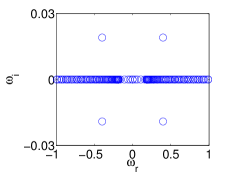
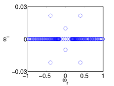
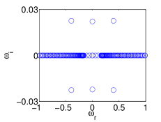
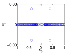
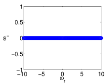
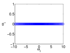
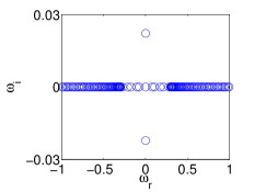
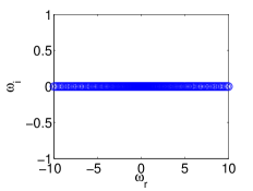
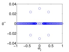
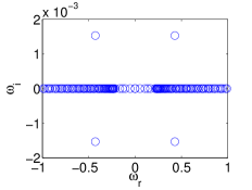
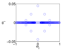
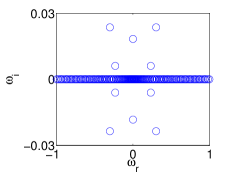
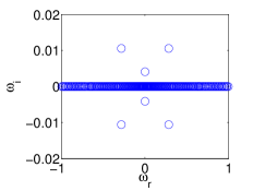
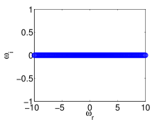
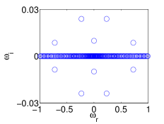
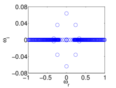
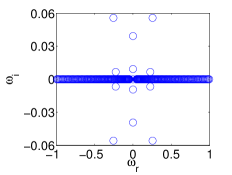
We investigate the stability of the steady states obtained by the Newton solvers at each continuation step, using linearized equations for small perturbations (see the Appendix). In particular, an eigenvalue problem [cf. Eq. (13)] is obtained (at order $\varepsilon$) and solved numerically afterward. The steady state is classified as a stable one if none of the eigenfrequencies $\omega=\omega_{r}+i\,\omega_{i}$ has a non-vanishing imaginary part $\omega_{i}$. Two types of instabilities can be thus identified: (i) exponential instabilities characterized by a pair of imaginary eigenfrequencies with zero real part and (ii) oscillatory instabilities characterized by a complex eigenfrequency quartet.

Finally, the spectral stability results obtained from the eigenvalue problem are checked against direct dynamical evolution of the coupled NLS system (1) forward in time. To this end, the Dormand-Prince method with an automatic time-step adaptation procedure (see the Appendix in Ref. Hairer ) and tolerance $10^{-13}$ is employed. We have also corroborated our results using the standard fourth-order Runge-Kutta method with a fixed time step of $\delta t=10^{-4}$, although numerical results are presented throughout this section using only the Dormand-Prince method. Thus, we initialize the dynamics at $t=0$ using the available steady states, with two distinct initialization approaches. We initialize the dynamics under the presence of a small (uniformly distributed) random perturbation with amplitude $10^{-3}$ for the class of stable steady states. An alternative approach is to initialize the dynamics using the linearization ansatz (12) for the unstable solutions with $\varepsilon=10^{-2}$ (except for the first excited antisymmetric steady state with $D=0.2$ and $\mu_{+}=0.77$, where $\varepsilon=10^{-1}$ is used) and eigenvector $\mathcal{V}$ corresponding to the (complex) eigenfrequency having the largest imaginary part. The latter approach is useful towards seeding the relevant instability and observing the ensuing dynamics.

III.2 Numerical results

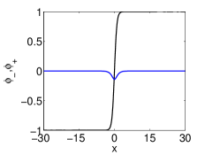
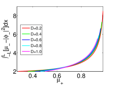
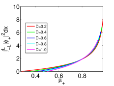
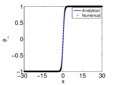
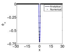
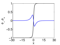
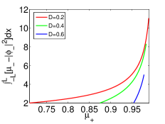
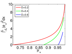
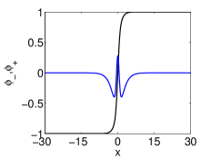
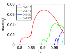
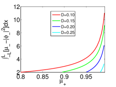
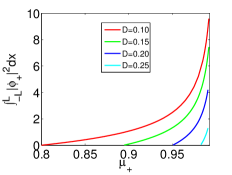
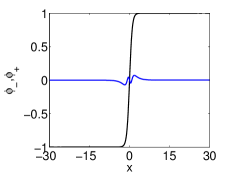
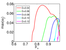
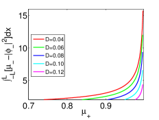
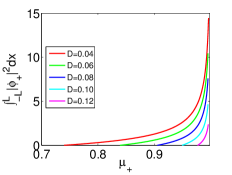
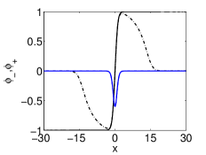
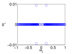
In this section, numerical results are presented for the coupled NLS system (1) and organized following the reasoning mentioned in the previous section. Figures 1-4 summarize the results for the existence of steady-state solutions and the corresponding parametric continuations (using $\mu_{+}$ as the continuation parameter, at different fixed values of $D$) for bound states of order $n=0$ (ground states with a single-hump bright component, corresponding to a generalization of the fundamental DB solitary waves), $n=1$ (the first excited odd states), $n=2$ (the second excited states, which are spatially even), and $n=3$ (the third excited states overall and second excited odd ones), respectively. Figures 1-4 present a typical example of the relevant profiles, while Figs. 1-4 showcase the growth rate of the most unstable perturbation mode $\textrm{max}(\omega_{i})$, which, if positive, indicates instability for the particular pair $(\mu_{+},D)$. Furthermore, Figs. 1-4 and 1-4 summarize the existence results by presenting

$$\int_{-L}^{L}\left[{\mu_{-}-|\phi_{-}(x)|^{2}}\right]{dx,~{}~{}}~{}~{}\int_{-L}^{L}{|\phi_{+}(x)|^{2}dx},$$ (11)

respectively, as functions of $\mu_{+}$ and for various fixed values of $D$. These integrals represent the total power in optics or the atom number in the BEC, considered as a function of the propagation constant or chemical potential, respectively.

Figure 1: (Color online) Bound states and continuation results corresponding to $n=0$ (i.e., the ground states). (a) Steady-state profiles of the dark (black line) and bright (blue line) soliton solutions for the parameters $D=1$ and $\mu_{+}=0.51$. (b) Maximal imaginary eigenfrequency as a function of the continuation parameter $\mu_{+}$ at various fixed values of $D$. (c) and (d) Solution norms, i.e., integral powers (11) associated with the solution branches, as functions of the continuation parameter $\mu_{+}$ at various fixed values of $D$. (e) Dark and (f) bright soliton solutions analytically predicted by Eq. (8) (blue line) and numerically obtained (black circles) for $D=0$ and $\mu_{+}=0.51$.

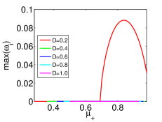
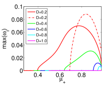
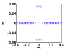
In particular, it can be inferred from Fig. 1 that solutions corresponding to the ground state are stable for $D=0.4-1.0$ and for all values of $\mu_{+}$ within the range of interest [see, e.g., Eq. (6) and the subsequent discussion]. In contrast, the solution branch corresponding to $D=0.2$ is stable up to a critical point $\mu_{+}^{\mathrm{crit}}\approx 0.69$, while past this value an exponential instability, accounted for by an imaginary eigenfrequency pair with zero real part, emerges [see also Fig. 7]. Similar arguments can be applied to Figs. 2-4, although the description is somewhat different. In particular, it can be seen in Fig. 2 that the solution branch corresponding to $D=0.2$ possesses a number of instability intervals for $\mu_{+}>0.71$. However, in the present case the instability is accounted for by a complex eigenfrequency quartet, which corresponds to an oscillatory instability related to a Hamiltonian Hopf bifurcation [see also Fig. 8 below as a case example]; for a recent discussion of relevant bifurcations, see, e.g., Ref. royg . While instabilities of this type are present as shown in Fig. 5, past the value of $\mu_{+}\approx 0.8252$ an additional imaginary eigenfrequency pair appears too, as depicted in Fig. 5 and initially marked with a dash-dotted red line in Fig. 2. As $\mu_{+}$ further increases, the exponentially unstable mode grows [cf. Fig. 5] and becomes dominant [cf. Fig. 5], while the oscillatory one follows a smaller growth rate, as depicted in Fig. 2 by a dash-dotted red line (the crossing of the solid line with the dash-dotted line marks the exchange of the dominant form of the instability). This is also the case for the solution branches with $D=0.4$ and $0.6$ depicted in Fig. 2 by dash-dotted green and blue lines, respectively. This transition between the exponentially and oscillatory unstable modes also occurs for the bound states of order $n=2$ [cf. Fig. 3] and $n=3$ [cf. Fig. 4]. An additional feature that arises in the latter figures is well known in the context of discrete systems as a finite-size effect and was introduced in Ref. kivshar . This is related to the fact that the continuous spectrum of background (phonon) excitations is discretized on our spatial grid, hence complex eigenfrequencies may return to the real eigenfrequency axis temporarily before colliding with another pair to exit again as quartets. It is expected (cf. Ref. kivshar ) that these discrete effects gradually disappear as the spectrum becomes denser, i.e., in the infinite-domain limit. It is the combination of the above-mentioned exchanges of the dominant instability type and of temporary restabilizations that gives rise to the spikes in Figs. 3 and 4. In such cases, only the dominant instability growth rate is shown; recall that Fig. 3 presents the results for the second excited (first excited even) branch and Fig. 4 those for the third excited (second excited odd) branch.

Figure 2: (Color online) Same as Fig. 1, but for bound states of order $n=1$ (i.e., first excited spatially odd states). (a) Steady-state profiles of the dark (black line) and bright (blue line) soliton solutions for $D=0.6$ and $\mu_{+}=0.96$. (b) Maximal imaginary eigenfrequency as a function of the continuation parameter $\mu_{+}$ at various fixed values of $D$. Notice that the second highest instability growth rates are also shown by dash-dotted lines (see the text for details). (c) and (d) Solution norms, given by integrals (11), as functions of the continuation parameter $\mu_{+}$ at various fixed values of $D$.

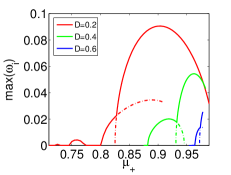
It is relevant to note that the branches with higher $n$ are generally more prone to instability than ones with lower $n$. The ground-state single-hump solution is generally fairly robust, as is suggested by the observability of the fundamental DB soliton in both atomic and optical settings sengdb ; peterprl ; peter1 ; seg1 . Our results reveal that only at very low values of $D$ does an instability arise for this state. On the other hand, branches with $n=1-3$ are less robust. Among them, our results suggest that the $n=1$ branch attains the highest instability growth rates. However, examining the parametric intervals of the instability (i.e., widths of the intervals of $\mu_{+}$ over which the branches remain stable), we observe that the higher the $n$, the narrower the corresponding stability interval becomes. Actually, the instability growth rates are relatively weak, typically $\sim 10^{-2}$, which suggests that the solutions should be long-lived ones, as the dynamical simulations corroborate below.

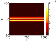
In a similar fashion, we also present results on steady-state solutions for bound states of order $n=0$ in Figs. 6 and 6 in the presence of the trapping potential in Eqs. (1a) and (1b) with $\Omega=0.1$. Specifically, Fig. 6 displays trapped DB soliton solutions (dash-dotted black and blue lines, respectively) which, according to our stability analysis, are fairly stable in the absence of the trap [cf. Fig. 1]. The naive intuition here would be that the trap would only contribute to the stability of the configuration. Yet exactly the opposite is happening here. In particular, deeper intuition suggests that the trap contributes to the breaking of the translational invariance of the system, releasing a negative-energy (negative-Krein-signature) mode along the imaginary axis of perturbation eigenvalues (see also the discussion in Ref. peter2 ). Upon variation of parameters, such as the chemical potential, this eigenvalue collides with other ones that correspond to positive energy, giving rise to instability quartets. Thus, while the $D=1$ case is, as is well known from previous studies of DB solitons in BECs (see, e.g.,  Refs.buschanglin ; peter2 ), generally stable, for other values of $D$, the setting with the trap is considerably less robust than in the homogeneous limit, where the translational invariance absorbs this potentially dangerous eigendirection. This scenario is depicted in Fig. 6, which complements the existence results presenting stability characteristics, namely, the dominant unstable eigenfrequency. Note that in Fig. 6 we include the $D=0.2$ branch of Fig. 1 denoted by a dash-dotted red line, for comparison.

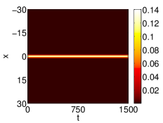
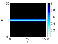
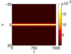
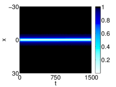
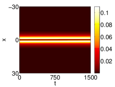
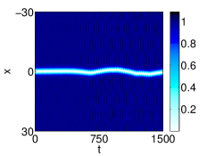
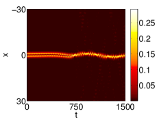
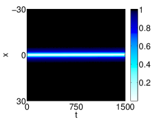
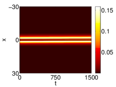
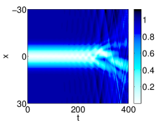
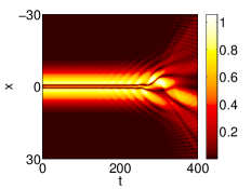
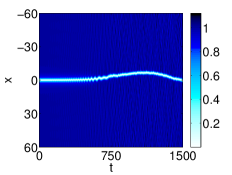
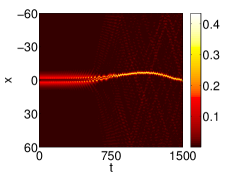
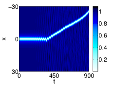
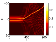
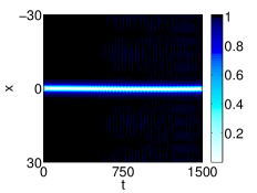
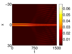
Finally, we present results on the evolution of perturbed steady-state solutions of orders $n=0,1,2,3$ (for various values of $D$ and $\mu_{+}$) in Figs. 7-10, respectively, while results corresponding to the bound state of order $n=0$ (with $D=0.2$) in the presence of the trapping potential are presented in Figs. 6-6 ($\mu_{+}=0.36$) and 6-6 ($\mu_{+}=0.8$). In particular, Figs. 6 and 6 and Figs. 6 and 6 correspond to the spatiotemporal evolution of the dark and bright components, respectively, while the corresponding eigenfrequency spectra of perturbations around the steady states (for which the evolution is examined) are presented in Figs. 6 and 6. For the stable steady states at hand [see Figs. 1-4], the corresponding dynamical evolution of the (a) dark and (b) bright components is depicted in the top rows of Figs. 7-10, respectively. In addition, the dynamical evolution of stable steady states in the presence of a harmonic trap is presented in Figs. 6-6 [see, in particular, Figs. 6 and 6]. Clearly, the stable solutions are indeed persistent, in the presence of small random perturbations, within the time range of the simulations.

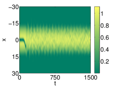
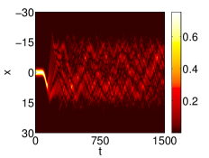
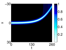
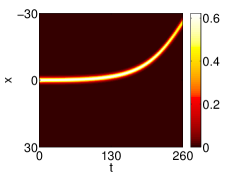
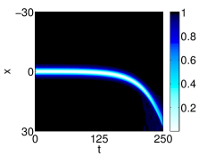
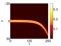
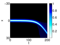
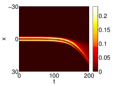
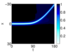
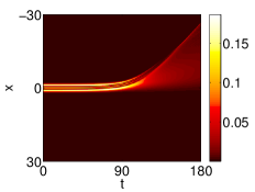
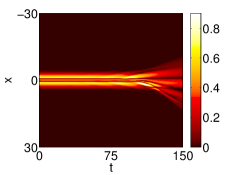
In contrast, a number of different scenarios are observed for unstable solutions, depending upon the corresponding dominant unstable eigenmode, as predicted by computations of the eigenfrequencies. Specifically, perturbations applied along the unstable eigendirection corresponding to an exponential eigenmode typically lead to solitons’ mobility. This is the case in Figs. 7, 7, 8, 8, 9, 9, 10, and 10 where motion of the solitons is observed. While for the fundamental branch this type of mobility may be persistent, for the higher excited states the acceleration induced by the instability eventually leads to a breakdown of the solution (an apparent merging of the dark-in-bright solitons therein njp_yan ), after a sufficiently long time has elapsed. In the presence of the trapping potential, in Fig. 6, the oscillatory instability displaces once again the solitary wave from its equilibrium position. However, here the large difference of $D$ from $1$ does not allow the resulting moving DB to oscillate in the trap (as it would at $D$ close to $1$ buschanglin ; peter1 ; peter2 ) but rather contributes to its rapid destruction upon interaction with the background.

Figure 3: (Color online) Same as Fig. 1, but for bound states of order $n=2$ (i.e., first excited spatially even states). (a) Steady-state profiles of the dark (black line) and bright (blue line) soliton solutions for $D=0.2$ and $\mu_{+}=0.9655$. (b) Maximal imaginary eigenfrequency as a function of the continuation parameter $\mu_{+}$ at various values of $D$. (c) and (d) Powers associated with the solution branches [see Eq. (11)] versus the continuation parameter $\mu_{+}$ at various values of $D$.

Figure 4: (Color online) Same as Fig. 1, but for bound states of order $n=3$ (i.e., second excited antisymmetric states). (a) Steady-state profiles of the dark (black line) and bright (blue line) soliton solutions for $D=0.12$ and $\mu_{+}=0.977$. (b) Maximal imaginary eigenfrequency as a function of the continuation parameter $\mu_{+}$ at various values of $D$. (c) and (d) are similar to Figs. 3 and 3.

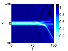
A number of additional possibilities emerge when unstable steady states are perturbed by oscillatory eigenmodes. This leads to oscillatory growth eventually translating into an apparent jerky motion of the corresponding dark and bright components. This behavior is presented in Figs. 8 and 8 (for $n=1$) [here it is clear that the instability wipes out the initial dark-in-bright solitary wave, transforming the bright component into a fundamental single-peak mode that is breathing in time]. Note also Figs. 9 and 9 (for $n=2$), where an explosion breaks apart the entire solitary wave. In Figs. 9 and 9 (i.e., for $n=2$), we observe a progression through the instability from a two-node solution in the bright component to a single-node one, and, eventually, to a fundamental state that is again breathing in time. In Figs. 10 and 10, a rapid destruction of the $n=3$ state occurs again, this time directly transforming it into a fundamental traveling-wave structure. In Figs. 10 and 10, a more complex scenario arises, with the dark soliton splitting off into apparently gray ones, the fastest of which is not accompanied by a bright counterpart. As a result, the bright component disperses, maintaining, however, some of its nodal structure. Finally, in Figs. 10 and 10 (once again, for $n=3$), the third excited state (the second spatially odd one) transforms itself into the corresponding first excited state maintaining, again, breathing oscillations.

It is worth noting that, for the fundamental branch, there is at most a translational (imaginary) eigenfrequency responsible for the instability. It is thus rather natural that its manifestation in direct simulations involves mobility. However, as we progressively move to higher excited states, the number of potentially unstable modes increases, creating an oscillatory instability for $n=1$, two instabilities for $n=2$, and so on, in accord with Figs. 8,  9, etc. It is the intricate interplay of these distinct dynamical instabilities (often with comparable growth rates) that is responsible for the resulting complex dynamics.

Figure 5: (Color online) Eigenfrequency spectra corresponding to bound states of order $n=1$ with $D=0.2$ and for (a) $\mu_{+}=0.82$, (b) $\mu_{+}=0.8257$, (c) $\mu_{+}=0.8277$, and (d) $\mu_{+}=0.8294$.

Figure 6: (Color online) Summary of results corresponding to $n=0$ (i.e., the ground states) in the presence of the trapping potential with $\Omega=0.1$. (a) Comparison of the steady-state profiles in the absence (solid lines) and presence (dash-dotted lines) of the trap. In particular, the dark (black) and bright (blue) soliton solutions are depicted for $D=0.2$ and $\mu_{+}=0.51$. (b) Maximal imaginary eigenfrequency as a function of the continuation parameter $\mu_{+}$ at various values of $D$; the dash-dotted red line corresponds to the $D=0.2$ branch of Fig. 1, for comparison. Also shown is the spatiotemporal evolution of densities $|\Phi_{-}(x,t)|^{2}$ (c) and (f) $|\Phi_{+}(x,t)|^{2}$ and (d) and (g) corresponding to perturbed soliton solutions, along with (e) and (h) the eigenfrequency spectrum of the steady states for (c)-(e) $D=0.2$ and $\mu_{+}=0.36$ and (f)-(h) $D=0.2$ and $\mu_{+}=0.8$.

Figure 7: (Color online) Spatiotemporal evolution of densities $|\Phi_{-}(x,t)|^{2}$ (a) and (d), and $|\Phi_{+}(x,t)|^{2}$ (b) and (e) corresponding to (perturbed) soliton solutions of order $n=0$, as well as the eigenfrequency spectra (c) and (f) of the steady states for (a)-(c) $D=1$ and $\mu_{+}=0.51$ and (d)-(f) $D=0.2$ and $\mu_{+}=0.7$.

Figure 8: (Color online) Same as in Fig. 7, but for soliton solutions of order $n=1$: spatiotemporal evolution of densities $|\Phi_{-}(x,t)|^{2}$ (a), (d), and (g), and $|\Phi_{+}(x,t)|^{2}$ (b), (e), and (h). Panels (c), (f), and (i) display the eigenfrequency spectra of the steady-state solutions for (a)-(c) $D=0.6$ and $\mu_{+}=0.96$, (d)-(f) $D=0.2$ and $\mu_{+}=0.83$, and (g)-(i) $D=0.2$ and $0.77$.

Figure 9: (Color online) Same as in Fig. 7, but for soliton solutions of order $n=2$: spatiotemporal evolution of densities $|\Phi_{-}(x,t)|^{2}$ (a), (d), (g), and (j), and $|\Phi_{+}(x,t)|^{2}$ (b), (e), (h), and (k). Panels (c), (f), (i), and (l) display the eigenfrequency spectra of the steady-state solutions for (a)-(c) $D=0.2$ and $\mu_{+}=0.9655$, (d)-(f) $D=0.1$ and $\mu_{+}=0.86$, (g)-(i) $D=0.1$ and $\mu_{+}=0.99$, and (j)-(l) $D=0.25$ and $\mu_{+}=0.99$.

Figure 10: (Color online) Same as in Fig. 7, but for soliton solutions of order $n=3$ and (a)-(c) $D=0.12$ and $\mu_{+}=0.977$, (d)-(f) $D=0.12$ and $\mu_{+}=0.99$, (g)-(i) $D=0.04$ and $\mu_{+}=0.8$, (j)-(l) $D=0.04$ and $\mu_{+}=0.95$, and (m)-(o) $D=0.06$ and $\mu_{+}=0.851$.

IV Conclusions

In the present work we have revisited the model based on two-component nonlinear Schrödinger equations with defocusing nonlinearity, which plays a fundamental role in nonlinear optics, as well as in the description of repulsively interacting binary BEC mixtures. We have examined the fundamental dynamical features of dark-bright solitons, namely, the formation of the effective potential well for the bright component induced by the dark one via the XPM interaction. Using the dispersion coefficient of the bright component as a control parameter, we modified the depth of the effective potential well, enabling the formation of higher-order excited bound states in this well, including those with $n=1,2$, and $3$ nodes. These may be considered as dark-in-bright solitary structures njp_yan or as excited states trapped in the potential well. We have shown that, while the ground single-peak state is generally very robust (except for the case of large difference between the dispersion coefficients of the two components), this is not true for the excited states, which are subject to progressively wider intervals of both exponential and oscillatory instabilities. The instability of the ground state leads to motion of the DB soliton, but does not destroy it. For the excited states with progressively increasing $n$, the complexity of the evolution scenarios also increases, resulting from the interplay of the increasing number of instability modes. Exotic scenarios involve the fusion of the dark-in-bright solitary waves, the explosion of the waveforms into multiple splinters, and relaxation, either abruptly or gradually, into less excited states, possibly accompanied by breathing.

The present analysis suggests a number of paths for future studies. One possibility might be to expand on the exact solutions identified herein for $D=0$ beyond this special limit, using a perturbative expansion to explore both their existence and, potentially, also their stability in the limit of small $D$. Moreover, one can extend the present considerations to the quite important (e.g., in BEC) and widely studied class of spinor systems, involving more than two components ueda_spin . Following this possibility, one can envision, in the spirit of Ref. DDB , one dark component creating a potential for the other two bright components, which could be found either in the same or, for suitable parametric regimes, possibly in different states of their respective potential wells. This would be a particularly intriguing setup to explore, as concerns its existence and stability properties. Furthermore, we note that the possibility of one component forming a well for another one is independent of the spatial dimension. For instance, in two dimensions the notion of vortex-bright solitons VB ; pola is a by-product of the same type of potential approach (the topological charge of the vortices is not experienced by the bright component when the interaction is incoherent, i.e., the potential well is solely determined by the density distribution in the vortex). Here it would be interesting to explore what type of excited states could be created, such as a dark-in-bright ring and associated multi ring states, inter alia.

ACKNOWLEDGMENTS

E.G.C. gratefully acknowledges financial support from the FP7-People Grant No. IRSES-605096 and thanks Hans Johnston (UMass Amherst) for providing computing facilities. The work of D.J.F. was partially supported by the Special Account for Research Grants of the University of Athens. P.G.K. acknowledges support from the National Science Foundation under Grants No. CMMI-1000337 and No. DMS-1312856, from FP7-People under Grant No. IRSES-605096, and from the U.S. AFOSR under Grant No. FA9550-12-10332. The work of P.G.K. and B.A.M. was supported in part by the U.S.-Israel Binational Science Foundation through Grant No. 2010239.

Appendix A The linearization ansatz and stability matrix

In this appendix we briefly discuss the linearization ansatz employed for the investigation of the stability of the stationary solutions, together with the formulation of the stability matrix. We start with the perturbation ansatz around stationary solutions $\phi_{\pm}^{0}(x)$ (which may be complex, in principle)

$$\widetilde{\Phi}_{-} = e^{-i\mu_{-}t}\Big{\{}\phi_{-}^{0}+\varepsilon\left[a(x)e^{i\omega t}+b^{\ast}(x)e^{-i\omega^{\ast}t}\right]\Big{\}},$$ (12a)

$$\widetilde{\Phi}_{+} = e^{-i\mu_{+}t}\Big{\{}\phi_{+}^{0}+\varepsilon\left[c(x)e^{i\omega t}+d^{\ast}(x)e^{-i\omega^{\ast}t}\right]\Big{\}},$$ (12b)

where $\omega$ is the (complex) eigenfrequency, $\varepsilon$ is a small amplitude of the perturbation, and the asterisk stands for complex conjugation. Then we insert Eqs. (12) into Eqs. (1) and thus obtain, at order $\varepsilon$, an eigenvalue problem in the following matrix form:

$$\rho\begin{pmatrix}a\\ b\\ c\\ d\end{pmatrix}=\begin{pmatrix}A_{11}&A_{12}&A_{13}&A_{14}\\ -A_{12}^{\ast}&-A_{11}&-A_{14}^{\ast}&-A_{13}^{\ast}\\ A_{13}^{\ast}&A_{14}&A_{33}&A_{34}\\ -A_{14}^{\ast}&-A_{13}&-A_{34}^{\ast}&-A_{33}\end{pmatrix}\begin{pmatrix}a\\ b\\ c\\ d\end{pmatrix},$$ (13)

with eigenvalues $\rho=-\omega$, eigenvectors $\mathcal{V}=(a,b,c,d)^{T}$, and matrix elements given by

$$A_{11} = -\frac{D_{-}}{2}\frac{\partial^{2}}{\partial x^{2}}+\gamma\left(2g_{11}|\phi_{-}^{0}|^{2}+g_{12}|\phi_{+}^{0}|^{2}\right)+V-\mu_{-},$$ (14a)

$$A_{12} = \gamma\,g_{11}\,\left(\phi_{-}^{0}\right)^{2},$$ (14b)

$$A_{13} = \gamma\,g_{12}\,\phi_{-}^{0}\left(\phi_{+}^{0}\right)^{\ast},$$ (14c)

$$A_{14} = \gamma\,g_{12}\,\phi_{-}^{0}\phi_{+}^{0},$$ (14d)

$$A_{33} = -\frac{D_{+}}{2}\frac{\partial^{2}}{\partial x^{2}}+\gamma\left(g_{12}|\phi_{-}^{0}|^{2}+2g_{22}|\phi_{+}^{0}|^{2}\right)+V-\mu_{+},$$ (14e)

$$A_{34} = \gamma\,g_{22}\,\left(\phi_{+}^{0}\right)^{2}.$$ (14f)

References

- (1) C. J. Pethick and H. Smith, Bose-Einstein Condensation in Dilute Gases (Cambridge University Press, Cambridge, 2002).
- (2) L. P. Pitaevskii and S. Stringari, Bose-Einstein Condensation (Oxford University Press, Oxford, 2003).
- (3) P. G. Kevrekidis, D. J. Frantzeskakis, and R. Carretero-González, Emergent Nonlinear Phenomena in Bose-Einstein Condensates: Theory and Experiment (Springer, Heidelberg, 2008).
- (4) R. Carretero-González, D. J. Frantzeskakis, and P. G. Kevrekidis, Nonlinearity 21, R139 (2008).
- (5) F. Kh. Abdullaev, A. Gammal, A. M. Kamchatnov, and L. Tomio, Int. J. Mod. Phys. B 19, 3415 (2005).
- (6) D. J. Frantzeskakis, J. Phys. A: Math. Theor. 43, 213001 (2010).
- (7) Yu. S. Kivshar and G. P. Agrawal, Optical Solitons: From Fibers to Photonic Crystals (Academic, San Diego, 2003).
- (8) M. J. Ablowitz, B. Prinari and A. D. Trubatch, Discrete and Continuous Nonlinear Schrödinger Systems (Cambridge University Press, Cambridge, 2004).
- (9) S. V. Manakov, Zh. Eksp. Teor. Fiz. 65, 505 (1973) [Sov. Phys. JETP 38, 248 (1974)].
- (10) Th. Busch and J. R. Anglin, Phys. Rev. Lett. 87, 010401 (2001).
- (11) H. E. Nistazakis, D. J. Frantzeskakis, P. G. Kevrekidis, B. A. Malomed, and R. Carretero-González, Phys. Rev. A 77, 033612 (2008).
- (12) M. Vijayajayanthi, T. Kanna, and M. Lakshmanan, Phys. Rev. A 77, 013820 (2008).
- (13) S. Rajendran, P. Muruganandam, M. Lakshmanan, J. Phys. B 42, 145307 (2009).
- (14) V. A. Brazhnyi and V. M. Pérez-García, Chaos Solitons Fractals 44, 381 (2011).
- (15) C. Yin, N. G. Berloff, V. M. Pérez-García, D. Novoa, A. V. Carpentier, and H. Michinel, Phys. Rev. A 83, 051605 (2011).
- (16) K. J. H. Law, P. G. Kevrekidis, and L. S. Tuckerman, Phys. Rev. Lett. 105, 160405 (2010).
- (17) A. Álvarez, J. Cuevas, F. R. Romero, and P. G. Kevrekidis, Physica D 240, 767 (2011).
- (18) V. Achilleos, P. G. Kevrekidis, V. M. Rothos, and D. J. Frantzeskakis, Phys. Rev. A 84, 053626 (2011).
- (19) V. Achilleos, D. Yan, P. G. Kevrekidis, and D. J. Frantzeskakis, New J. Phys. 14, 055006 (2012).
- (20) C. Becker, S. Stellmer, P. Soltan-Panahi, S. Dörscher, M. Baumert, E.-M. Richter, J. Kronjäger, K. Bongs, and K. Sengstock, Nat. Phys. 4, 496 (2008).
- (21) C. Hamner, J. J. Chang, P. Engels, M. A. Hoefer, Phys. Rev. Lett. 106, 065302 (2011).
- (22) S. Middelkamp, J. J. Chang, C. Hamner, R. Carretero-González, P. G. Kevrekidis, V. Achilleos, D. J. Frantzeskakis, P. Schmelcher, and P. Engels, Phys. Lett. A 375, 642 (2011).
- (23) D. Yan, J. J. Chang, C. Hamner, P. G. Kevrekidis, P. Engels, V. Achilleos, D. J. Frantzeskakis, R. Carretero-González, and P. Schmelcher, Phys. Rev. A 84, 053630 (2011).
- (24) M. A. Hoefer, J. J. Chang, C. Hamner, and P. Engels, Phys. Rev. A 84, 041605 (2011).
- (25) D. Yan, J. J. Chang, C. Hamner, M. A. Hoefer, P. G. Kevrekidis, P. Engels, V. Achilleos, D. J. Frantzeskakis, and J. Cuevas, J. Phys. B 45, 115301 (2012).
- (26) Z. Chen, M. Segev, T. H. Coskun, D. N. Christodoulides, Yu. S. Kivshar, and V. V. Afanasjev, Opt. Lett. 21, 1821 (1996).
- (27) E. A. Ostrovskaya, Yu. S. Kivshar, Z. Chen, and M. Segev, Opt. Lett. 24, 327 (1999).
- (28) Z. Chen, M. Segev, T. H. Coskun, D. N. Christodoulides, and Yu. S. Kivshar, J. Opt. Soc. Am. B 14, 3066 (1997).
- (29) F. Tsitoura, V. Achilleos, B. A. Malomed, D. Yan, P. G. Kevrekidis, and D. J. Frantzeskakis, Phys. Rev. A 87, 063624 (2013).
- (30) V. Achilleos, D. J. Frantzeskakis, and P. G. Kevrekidis Phys. Rev. A 89, 033636 (2014).
- (31) J. Dalibard, F. Gerbier, G. Juzeliünas, and P. Öhberg, Rev. Mod. Phys. 83, 1523 (2011).
- (32) V. M. Pérez-García and J. B. Beitia, Phys. Rev. A 72, 033620 (2005); S. K. Adhikari, Phys. Lett. A 346, 179 (2005); Phys. Rev. A 72, 053608 (2005).
- (33) L. D. Landau and E. M. Lifshitz, Quantum Mechanics (Nauka, Moscow, 1989).
- (34) G. Pöschl, E. Teller, Z. Phys. 83, 143 (1933).
- (35) C. T. Kelley, Solving Nonlinear Equations with Newton’s Method (SIAM, Philadelphia, 2003).
- (36) A. H. Nayfeh and B. Balachandran, Applied Nonlinear Dynamics: Analytical, Computational and Experimental Methods (Wiley, New York, 1995).
- (37) E. Hairer, S. P. Nørsett and G. Wanner, Solving ordinary differential equations I (Springer, Berlin, 1993).
- (38) R. H. Goodman, J. Phys. A: Math. Theor. 44, 425101 (2011).
- (39) M. Johansson and Yu. S. Kivshar, Phys. Rev. Lett. 82, 85 (1999).
- (40) P. G. Kevrekidis, D. J. Frantzeskakis, B. A. Malomed, A. R. Bishop and I. G. Kevrekidis New J. Phys. 5, 64 (2003).
- (41) D. M. Stamper-Kurn and M. Ueda Rev. Mod. Phys. 85, 1191 (2013).
- (42) M. Pola, J. Stockhofe, P. Schmelcher, and P. G. Kevrekidis Phys. Rev. A 86, 053601 (2012).