models for random hypergraphs with a given degree sequence
Abstract
We introduce the beta model for random hypergraphs in order to represent the occurrence of multi-way interactions among agents in a social network. This model builds upon and generalizes the well-studied beta model for random graphs, which instead only considers pairwise interactions. We provide two algorithms for fitting the model parameters, IPS (iterative proportional scaling) and fixed point algorithm, prove that both algorithms converge if maximum likelihood estimator (MLE) exists, and provide algorithmic and geometric ways of dealing the issue of MLE existence.
1 Introduction
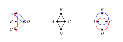
Social network models [8] are statistical models for the joint occurrence of random edges in a graph, as a means to model social interactions among agents in a population of interest. These models typically focus on representing only binary relations between individuals. As a result, when one is interested in higher-order (-ary) interactions, statistical models based on graphs may be ineffective or inadequate. Examples of -ary relations are plentiful, and include forum or committee membership, co-authorship on scientific papers, or proximity of groups of people in photographs. These datasets have been studied by replacing each -dimensional group with a number of binary relations (in particular, of them, which form a clique), thus extracting binary information from the data, and then modeling and studying the resulting graph. Such a process inevitably causes information loss. For instance, let us consider statisticians Adam (), Barbara (), Cassandra (), and David (), see Figure 1. Suppose the authors wrote three papers in following groups: , , . Representing this information as a graph with edges between any two individuals who have co-authored a paper provides a graph with edges . A hypergraph representing this information would instead use the exact groups as hyperedges and, unlike , would be able to represent additional properties of such interactions, including how many papers were coauthored by these four individuals; see Figure 1. If, in addition, is more likely to write a 3-author paper than a 2-author paper, this requires modeling separately the probabilities of these collaborations. Despite the growing needs of practical values, models for random hypergraphs are relatively few and simple. Random hypergraphs have been studied ([7]) as generalizations of the simple Erdös-Rényi model [4] for networks; [5] considers an application of random tripartite hypergraphs to Flickr photo-tag data.
In this paper we introduce a simple and natural class of statistical models for random hypergraphs, which we term hypergraph beta models, that allows one to model directly simultaneous higher-order (and not only binary) interactions among individuals in a network. As its name suggests, our model arises as a natural extension of the well-studied beta model for random graphs, the exponential family for undirected networks which assumes independent edges and whose minimal sufficient statistics vector is the degree sequence of the graph. It is a special class of the more general of models [6] which assume independent edges and parametrize the probability of each edge by the propensity of the two endpoint nodes. This model has been studied extensively; see [2, 3, 9, 10, 11], which give, among other results, methods for model fitting.
Below we formalize the class of the beta models for hypergraphs. Just like the graph beta model, these are natural exponential random graph models over hypergraphs which postulate independent edges and whose sufficient statistics are the (hypergraph) degree sequences. Our contributions are two-fold: first we formalize three classes of linear exponential families for random hypergraphs of increasing degree of complexity and derive the corresponding sufficient statistics and moment equations for obtaining the maximum likelihood estimator (MLE) of the model parameters. Secondly, we design two iterative algorithms for fitting these models that do not require evaluating the gradient or Hessian of the likelihood function and can therefore be applied to large data: a variant of the IPS algorithm and a fixed point iterative algorithm to compute the MLE of the edge probabilities and of the natural parameters, respectively. We show that both algorithms will converge if the MLE exists. Finally, we illustrate our results and methods with some simulations.
As our analysis reveals, the study of the theoretical and asymptotic properties of hypergraph beta models is especially challenging, more so than with the ordinary beta model. The complexity of the new models, in turn, leads to the problem of optimizing a complex likelihood function. Indeed, when the MLE does not exist, optimizing the likelihood function becomes highly non-trivial and, to a large extent, unsolved for our model as well as for many other discrete linear exponential families. To this end, we describe a geometric way for dealing with the issue of existence of the MLE for these models and gain further insights into this difficult problem with simulation experiments.
2 The hypergraph beta model: three variants
A hypergraph is a pair , where is a set of nodes (vertices) and is a family of non-empty subsets of of cardinality different than ; the elements of are called the hyperedges (or simply edges) of . In a -uniform hypergraph, all edges are of size . We restrict ourselves to the set of hypergraphs on nodes, where nodes have a distinctive labeling. Let be the set of all realizable hyperedges for a hypergraph on nodes. While can in principle be the set of all possible hyperedges, below we will consider more parsimonious models in which is restricted to be a structured subset of edges. Thus we may write a hypergraph as the zero/one vector , where for and for . The degree of a node in is the number of edges it belongs to; the degree information for is summarized in the degree sequence vector whose th entry is the degree of node in .
Hypergraph beta models are families of probability distributions over which postulate that the hyperedges occur independently. In details, let be a vector of probabilities whose th coordinate indicates the probability of observing the hyperedge . We will assume . Every such vector parametrizes a beta-hypergraph model as follows: the probability of observing the hypergraph is
| (1) |
The graph beta model is a simple instance of this model, with . The edge probabilities are parametrized as , for and some real vector .
Various social network modeling considerations for node interactions require a flexible class of models adaptable to those settings. Thus, we introduce three variants of the beta model for hypergraphs with independent edges in the form of linear exponential families: beta models for uniform hypergraphs, for general hypergraphs, and for layered uniform hypergraphs. For each, we provide an exponential family parametrization in minimal form and describe the corresponding minimal sufficient statistics.
Uniform hypergraphs.
The probability of a size- hyperedge appearing in the hypergraph is parametrized by a vector as follows:
| (2) |
with for all . In terms of odds ratios,
| (3) |
In order to write the model in exponential family form, we abuse notation and define for each hyperedge , . In addition, let be the set of all subsets of size of the set . By using (1), we obtain
where is the degree of the node in . Then it is clear that the sufficient statistics for the uniform beta model are the entries of the degree sequence vector of the hypergraph, , and the normalizing constant is
| . | (4) |
Layered uniform hypergraphs.
Allowing for various size edges has the advantage of controlling the propensity of each individual to belong to a size- group independently for distinct ’s. Let be the (natural bound for the) maximum size of a hyperedge that appears in . This model is then parametrized by vectors in as follows:
where, for each , . There are parameters in this parametrization. By using (1) again, we obtain
where is the number of hyperedges of size to which node belongs in . Notice that the vector of sufficient statistics in this case is , and the normalizing constant is
| . | (5) |
General hypergraphs.
In the third variant of the model we define one parameter for each node, controlling the propensity of that node to be in a relation of any size. The probability of observing a hypergraph is thus
The vector of sufficient statistics is then , where , and the normalizing constant is .
3 Parameter estimation
Iterative proportional scaling algorithms.
From the theory of exponential families, it is known that the MLE satisfies the following system of equations:
| (6) |
where is the average observed degree sequence. By using (4), we then obtain
| (7) |
which is itself equivalent to , for .
Iterative proportional scaling (IPS) algorithms fit the necessary margins of a provided table, whose elements correspond to the mean-value parameters (in this case probabilities of observing an edge). We design the following IPS algorithm for computing .
Algorithm 3.1.
Define to be an -way table with margins for all its layers. Set the following structural zeros on the table: if for at least one pair , . (Note that there are non-zero elements in the table.) Place on all other elements of the matrix, where . Then apply the following iterative st step for every element : where .
IPS algorithms are known to converge to elements of the limiting matrix () which are unique and preserve all the marginals (see e.g. [1]). Solving the system (3) for every provides . Algorithm 3.1 can be adjusted for layered uniform and general hypergraph beta models.
For layered -uniform hypergraphs, by using (12) and (5) we obtain for and ,
| (8) |
Therefore, we can apply Algorithm 3.1 to -way tables similar to those of the -uniform case, where ranges from to .
For general hypergraphs, we similarly obtain
| (9) |
In this case we apply the IPS algorithm to the following table: Define to be a -way table of size consisting of labels with margins for all its layers, where does not need to be known or calculated. We also set the following structural zeros in the table: if (1) for at least one pair , ; (2) except possibly for one . We apply Algorithm 3.1 as in the -uniform case except the fact that we do not fit the margins. We read the elements of the limiting matrix of from, as , which corresponds to a lower dimensional probability.
Fixed Point Algorithms.
An alternative method for computing MLE is based on [3]. In the -uniform case, for , Equation (7) can be rewritten as
| (10) |
Therefore, in order to find , it is sufficient to find the fixed point of the function .
Algorithm 3.2.
Start from any and define for .
Theorem 3.3.
If the MLE exists, Algorithm 3.2 converges geometrically fast; if the MLE does not exist there is a diverging subsequence in .
The proof is omitted due to space limitations. For the other models, the above theory can be easily generalized. For the layered models and general hypergraph models, we apply the same algorithm to obtain the fixed points of the following functions respectively for and and .
| (11) | |||||
| (12) |
4 Simulations and Analysis
MLE.
We use the fixed point algorithm to estimate the natural parameters for hypergraph beta models, examine non-existence of MLE and compare the layered and general variants of the model on simulated data. Note that most dense hypergraphs, when reduced to binary relations give the complete graph, for which the MLE does not exist. In contrast, MLE is expected to exist for the hypergraph beta model in this case.
Example 4.1.
We simulate a hypergraph drawn from the beta model for -uniform hypergraphs on vertices with . The average simulated degree sequence of hypergraphs drawn from this model is and the average simulated density of the corresponding hypergraph is 0.33. Algorithm 3.2 provides the following MLE estimate using as the sufficient statistic: . Note that .
For a larger example, we select a value giving rise to -uniform hypergraphs on vertices with density , and obtain a closer estimate: .
Example 4.2.
Theorem 3.3 guarantees that if is the solution to the ML equations (10), (12), or (12), then the sequence of -estimates that the fixed point algorithm produces will converge to ; else there will be a divergent subsequence. To detect a divergent sequence in practice, we either look for a periodic subsequence, or for a number with large absolute value in the sequence that seems to be growing, sometimes quite slowly. From (2), since converges to quickly (), for graphs with small number of nodes (i.e. far from the asymptotic behavior), it is plausible to conclude that the corresponding mean value parameter is approximately or , and hence the MLE does not exist. Figure 2 demonstrates MLE existence against edge densities for random hypergraphs with a fixed edge-density. Interestingly, in this restricted class, our simulations give evidence of a transition from non-existence of the MLE to existence as the density of the hypergraphs increases. The transition point seems to depend on both the number of vertices and the edge sizes allowed in the model.

|

|

|

|

|

|
Model fitting: Layered versus general hypergraph beta models.
Consider the two variants of the beta model for non-uniform hypergraphs: the general model, with one parameter per node , and the layered model, with one parameter per node and edge size . Since the former can be considered a submodel of the latter by setting certain constraints on , , we compare the fit of these two models using the likelihood ratio test with test statistics . Our experiments indicate that the layered model fits significantly better than the general case. Using 100 random sequences on 10 vertices, with allowed edge-sizes 2 and 3, we obtain the average observed test statistics , in the critical region for significance level, , for chi-square with degrees of freedom. The layered model fits significantly better for significance level 0.05 in all 100 cases, and 97 and 94 times better for significance levels 0.01 and 0.005, respectively.
References
-
[1]
Y. M. M. Bishop, S. E. Fienberg, and P. W. Holland.
Discrete Multivariate Analysis: Theory and Practice.
MIT Press, Cambridge, Mass.-London, 1975.
-
[2]
J. Blitzstein and P. Diaconis.
A sequential importance sampling algorithm for generating random
graphs with prescribed degrees.
Available at www.people.fas.harvard.edu/~blitz/BlitzsteinDiaconisGraphAlgorithm.pdf, 2009.
-
[3]
Sourav Chatterjee, Persi Diaconis, and Allan Sly.
Random graphs with a given degree sequence.
The Annals of Applied Probability, 21(4):1400–1435, 2011.
-
[4]
P. Erdös and A. Rényi.
On random graphs.
Publicationes Mathematicae, 6:290–297, 1959.
-
[5]
Gourab Ghoshal, Vinko Zlatic, Guido Caldarelli, M. E. J. Newman.
Random hypergraphs and their applications, 2009.
http://arxiv.org/abs/0903.0419.
-
[6]
Paul Holland, Samuel Leinhardt.
An exponential family of probability distributions for directed
graphs.
Journal of the American Statistical Association,
76:33–50, 1981.
-
[7]
Michal Karonski and Tomasz Luczak.
The phase transition in a random hypergraph.
Journal of Computational and Applied Mathematics,
142:125—135, 2002.
-
[8]
Erik Koladzyk: (2009): Statistical Analysis of Network Data: Methods and Models. Springer Series in Statistics
-
[9]
Alessandro Rinaldo, Sonja Petrović, and Stephen E. Fienberg.
Maximum lilkelihood estimation in the beta model.
Annals of Statistics, 41(3):1085–1110,
2013.
-
[10]
T Yan, J Xu, and Y Yang.
High dimensional Wilks phenomena in random graph models.
Available at http://arxiv.org/abs/1201.0058, 2012.
-
[11]
T Yan and J Xu.
A central limit theorem in the -model for undirected random
graphs with a diverging number of vertices.
Available at http://arxiv.org/abs/1202.3307, 2012.