Resolving kinematic ambiguities in QCD predictions for Deeply Virtual Compton Scattering

Abstract:

The existing QCD predictions for the Deeply Virtual Compton Scattering (DVCS) depend on the convention used for the skewedness parameter and on the reference frame used to define helicity amplitudes. These ambiquities are formally power-suppressed but numerically significant. They are cancelled by finite-$t$ and target mass corrections that have been calculated recently to the $1/Q^{2}$ accuracy. It turns out that these corrections can be minimized, at least for unpolarized observables, by choosing a specific reference frame where longitudinal directions are defined by the photon momenta.

Deeply Virtual Compton Scattering (DVCS) is the simplest process that gives access to generalized parton distributions (GPDs) and is receiving a lot of attention. The existing experimental results come from DESY (HERA H1, ZEUS and HERMES) and Jefferson Lab (Hall A and CLAS) and many more measurements are planned after the Jefferson Lab $12$ GeV upgrade and at COMPASS-II at CERN. The standard theoretical framework is based on collinear factorization which is proven in QCD to the leading power accuracy in the photon virtuality $Q$. This approach, commonly referred to as the leading twist (LT) approximation, appears to be sufficient to describe main features of the available data raising the hope that a fully quantitative description is within reach. The future data will have much higher statistics and allow one to extract at least some GPDs with controllable precision.

The LT approximation is, however, incomplete and in fact convention-dependent. It is well known that the LT DVCS amplitudes do not satisfy electromagnetic Ward identities. The Lorentz (translation) invariance is violated as well: The results depend on the frame of reference chosen to define the skewedness parameter and the helicity amplitudes. The required symmetries are restored by a subset of higher-twist, i.e power-suppressed, corrections $\sim t/Q^{2}$ and $\sim m^{2}/Q^{2}$ that can be called kinematic as they are expressed in terms of the same GPDs that enter the LT amplitudes, i.e. they do not involve new nonperturbative input. One expects that the subset of kinematical power corrections is factorizable for arbitrary twist. The structure of kinematic corrections turns out to be nontrivial and was understood only recently [1, 2, 3, 4]. The first detailed study of their impact on various DVCS observables is presented in [5].

The reason why the LT approximation is intrinsically ambiguous is that in the DVCS kinematics the four-momenta of the initial and final photons and protons do not lie in one plane. Hence the distinction of longitudinal and transverse directions is convention-dependent. In the Bjorken high-energy limit this is a $1/Q$ effect. The freedom to redefine large ‘plus’ parton momenta by adding smaller transverse components has two consequences. First, the relation of the skewedness parameter $\xi$ appearing as an argument in GPDs to the Bjorken variable $x_{B}$ may involve power suppressed contributions. Second, such a redefinition generally leads to excitation of the subleading photon helicity-flip amplitudes. Any attempt to compare the calculations with and without kinematic power corrections must start with specifying the precise conventions, i.e. the definition of what is meant by ‘leading-twist’ to the power accuracy. This is an important point that is often overlooked in phenomenological studies.

The common wisdom is that at leading order (LO) and the LT level there are four Compton form factors (CFFs) ${\mathcal{F}}\in\{{\mathcal{H}},{\mathcal{E}},\widetilde{\mathcal{H}},\widetilde{\mathcal{E}}\}$ that are given by convolution integrals of GPDs $F\in\{H,E,\widetilde{H},\widetilde{E}\}$ over the momentum fraction $x$ with simple coefficient functions,

$${\mathcal{F}} \stackrel{{\scriptstyle\rm LO}}{{=}}\sum_{q}e_{q}^{2}\int_{-1}^{1}\!\!\frac{dx}{2\xi}\,T_{0}\biggl{(}\!\frac{\xi+x-i\epsilon}{2(\xi-i\epsilon\!)}\biggr{)}F^{q^{(+)}}(x,\xi,t)\,~{}\stackrel{{\scriptstyle\rm LO}}{{\equiv}}T_{0}\!\circledast\!F\,, T_{0}(u)=\frac{1}{1-u}$$ (1)

with an obvious correspondence ${\mathcal{H}}\leftrightarrow H\,,\;\;{\mathcal{E}}\leftrightarrow E\,,\;\;\widetilde{\mathcal{H}}\leftrightarrow\widetilde{H}\,,\;\;\widetilde{\mathcal{E}}\leftrightarrow\widetilde{E}\,.$ Here and below $F\equiv F^{q^{(+)}}(x,\xi,t)$ are the $C=+1$ combinations of the GPDs defined with the established conventions, and we have introduced a notation ‘$\circledast$’ for the (normalized) convolution integral, including the sum over the quark flavors.

If the QCD calculation is done to the ${1/Q^{2}}$ accuracy, the following complications occur and must be taken into account: a) The skewedness parameter $\xi$ must be defined with a power accuracy

$$\xi\to\xi(x_{B},t,Q^{2})=\frac{x_{B}}{2-x_{B}}+\mathcal{O}(1/Q^{2})\,,$$ (2)

b) The CFFs must be defined through a certain decomposition of the DVCS tensor. The LO CFFs (1) are recovered as the scaling limit of the helicity-conserving CFFs, that is

$${}\hskip 17.07182pt\mathcal{F}_{++} =T_{0}\!\circledast\!F\Big{|}_{\xi\to\xi(x_{B},t,Q^{2})}+\mathcal{O}(1/Q,1/Q^{2}),$$ (3)

where the expression for the $\mathcal{O}(1/Q,1/Q^{2})$ addenda depends both on the chosen form factor decomposition and on the convention used for the skewedness parameter. c) There are eight more CFFs $\mathcal{F}_{0+},\mathcal{F}_{-+}$ corresponding to photon helicity flip transitions that must be taken into account in the same approximation. The existing freedom in definitions is related to the choice of the reference frame in which one performs the calculation. It is important to realize that the corresponding ambiguities only cancel at the level of physical observables.

One possibility is to use a certain generalization of the standard DIS reference frame where the initial photon and proton momenta form the longitudinal plane. In the Belitsky, Müller and Ji (BMJ) reference frame [6, 7, 8] the nucleon target is at rest, $p_{1}^{\mu}=(m,0,0,0)$, and the incoming photon momentum is specified as $q_{1}^{\mu}=({Q}/{\gamma})\bigl{(}1,0,0,-\sqrt{1+\gamma^{2}}\bigr{)}$ with $\gamma\equiv\epsilon^{\rm BMJ}={2mx_{\rm B}}/{Q}$. The polarization vectors of the initial photon are defined as $\epsilon_{1}^{\mu}(0)=({1}/{\gamma})\bigl{(}-\sqrt{1+\gamma^{2}},0,0,1\bigr{)}$ and $\epsilon_{1}^{\mu}(\pm)=({e^{\mp i\phi}}/{\sqrt{2}})\bigl{(}0,1,\pm i,0\bigr{)}$, where the phase is given by the azimuthal angle $\phi$ of the final state nucleon. BMJ employ the KM convention for the skewedness variable $\xi(x_{\rm B},t,Q^{2})=\xi_{\rm KM}={x_{\rm B}}/(2-x_{\rm B})$, used by Kumerički and Müller in global DVCS fits [9, 10]. A complete parametrization of the Compton tensor in terms of CFFs in this frame was proposed in Ref. [6]. Starting from this parametrization, the electroproduction cross section has been calculated [7, 8] (BMJ) for all possible polarization options of the initial electron and nucleon.

In contrast to this traditional approach, Braun, Manashov and Pirnay (BMP) [3, 4] define the longitudinal plane as spanned by the two photon momenta $q_{1}$ and $q_{2}$. For this choice the momentum transfer to the target $\Delta=q_{1}-q_{2}$ is purely longitudinal and both — initial and final state — protons have the same nonvanishing transverse momentum $P_{\perp}$, such that $|\xi P_{\perp}|^{2}=(1/4)(1-\xi^{2})(t_{\rm min}-t)\,,\quad t_{\rm min}=-4m^{2}\xi^{2}/(1-\xi^{2})\,,$ where $\xi=\xi_{\rm BMP}$ is the BMP skewedness parameter defined with respect to the real (final state) photon momentum $q_{2}^{2}=0$: $\xi_{\rm BMP}=x_{\rm B}(1+t/Q^{2})/[2-x_{\rm B}(1-t/Q^{2})].$ The main advantage of this choice is that polarization of both the initial and the final photon can be described using the same polarization vectors, see Appendix A in Ref. [5], that allows to obtain a comparatively simple Lorentz-decomposition of the Compton tensor in terms of the CFFs.

The BMP CFFs ${\mathfrak{F}}\in\{{\mathfrak{H}},{\mathfrak{E}},\widetilde{\mathfrak{H}},\widetilde{\mathfrak{E}}\}$ are, however, different from their BMJ analogues ${\mathcal{F}}\in\{{\mathcal{H}},{\mathcal{E}},\widetilde{\mathcal{H}},\widetilde{\mathcal{E}}\}$. The relation can easily be worked out [5]:

$${\mathcal{F}}_{\pm+}={\mathfrak{F}}_{\pm+}+\frac{\varkappa}{2}\Big{[}{\mathfrak{F}}_{++}+{\mathfrak{F}}_{-+}\Big{]}-\varkappa_{0}\,{\mathfrak{F}}_{0+}, {\mathcal{F}}_{0+}=-\left(1+\varkappa\right){\mathfrak{F}}_{0+}+\varkappa_{0}\Big{[}{\mathfrak{F}}_{++}+{\mathfrak{F}}_{-+}\Big{]}$$ (4)

with an obvious correspondence ${\mathcal{H}}\leftrightarrow{\mathfrak{H}}$, etc. Explicit expressions for the kinematic factors $\varkappa_{0}=\mathcal{O}(1/Q)$ and $\varkappa=\mathcal{O}(1/Q^{2})$ are given in Eq. (48) in [5]. Using the exact transformation formulas from the BMP to the BMJ basis, Eq. (4), one can calculate physical observables from the expressions given in Ref. [8]. In this way the results are the same as the corresponding results which one would obtain by a direct calculation by means of the original BMP parametrization.

Within the BMJ conventions, the LT approximation to LO accuracy can be summarized as:

$$\text{LT}\equiv\text{LT}_{\rm KM} :~{}\begin{cases}{\mathcal{F}}_{++}=T_{0}\!\circledast\!F,&{\mathcal{F}}_{0+}=0\\ {\mathcal{F}}_{-+}=0,&\xi=\xi_{\rm KM}\end{cases}$$ (5)

i.e. the BMJ helicity-conserving CFF is calculated in the LO approximation using $\xi_{\rm KM}=x_{B}/(2-x_{B})$ for the skewedness parameter and the other CFFs are put to zero. This ansatz [10] in practical terms is not very different from the VGG convention used by Guidal, and also the convention used by Kroll, Moutarde and Sabatie in [11].

Starting instead from the BMP framework, the analogous LT and LO approximation, rewritten in terms of the BMJ CFFs using the transformation rules in (4), reads

$$\text{LT}_{\rm BMP} :~{}\begin{cases}{\mathcal{F}}_{++}=\left(\!1+\frac{\varkappa}{2}\!\right){\mathfrak{F}}_{++}\,,&{\mathcal{F}}_{0+}=\varkappa_{0}\,{\mathfrak{F}}_{++}\\[2.84526pt] {\mathcal{F}}_{-+}=\frac{\varkappa}{2}{\mathfrak{F}}_{++},&\xi=\xi_{\rm BMP}\,.\end{cases}$$ (6)

The two LT ansätze in Eq. (5) and Eq. (6) are both perfectly legitimate. Their difference reveals that both the distinction between helicity-conserving and helicity-flip CFFs, and the expression for skewedness parameter in terms of kinematic invariants, depend to power $1/Q$ accuracy on the reference frame. The resulting ambiguity is quite large because, first, the kinematic factors $\varkappa_{0}$ and $\varkappa$ are sizable despite of being power-suppressed. For example, for $-t/Q^{2}\simeq 1/4$ one obtains $\varkappa/2\sim 1/3$. Second, $\xi_{\rm BMP}<\xi_{\rm KM}$, for practical purposes one can approximate $\xi_{\rm BMP}\approx(1+t/Q^{2})\xi_{\rm KM}$ for $x_{\rm B}\leq 0.4$. Thus generally $F(\xi_{\rm BMP},\xi_{\rm BMP})>F(\xi_{\rm KM},\xi_{\rm KM})$ if the GPDs have Regge behavior, although this effect is moderated for larger $t$ by the slope of the Regge-trajectory.

This ambiguity is resolved by adding kinematic power corrections to the Compton amplitude that correspond to contributions of higher-twist operators of special type, obtained from the LT operators by adding total derivatives [1, 2]. The same contributions restore electromagnetic gauge invariance and translation invariance of the results. To the $\mathcal{O}(1/Q^{2})$ accuracy one obtains [4, 5], e.g. for ${\mathfrak{H}}_{ab}$ CFFs in the BMP basis:

$${\mathfrak{H}}_{++} ={T}_{0}\circledast H+\frac{t}{Q^{2}}\Big{[}-\frac{1}{2}{T}_{0}+{T}_{1}+2\xi\mathbb{D}_{\xi}\,{T}_{2}\Big{]}\circledast H+\frac{2t}{Q^{2}}\xi^{2}\partial_{\xi}\xi{T}_{2}\circledast M\,,$$

$${\mathfrak{H}}_{0+} =-\frac{4|\xi P_{\perp}|}{\sqrt{2}Q}\Big{[}\xi\partial_{\xi}{T}_{1}\circledast H+\frac{t}{Q^{2}}\partial_{\xi}\xi\,{T}_{1}\circledast M\Big{]}-\frac{t}{\sqrt{2}Q|P_{\perp}|}{T}_{1}\circledast\Big{[}\xi\,M-\widetilde{H}\Big{]}\,,$$ (7)

$${\mathfrak{H}}_{-+} =\frac{4|\xi P_{\perp}|^{2}}{Q^{2}}\Big{[}\xi\partial^{2}_{\xi}\xi\,T_{1}^{(+)}\circledast H+\frac{t}{Q^{2}}\partial^{2}_{\xi}\xi^{2}\,T_{1}^{(+)}\circledast M\Big{]}+\frac{2t}{Q^{2}}\xi\Big{[}\xi\partial_{\xi}\xi\,T_{1}^{(+)}\circledast M+\partial_{\xi}\,\xi\,T_{1}\circledast\widetilde{H}\Big{]},$$

where $M=H+E$, $\mathbb{D}_{\xi}=\partial_{\xi}+(2/t){|\xi P_{\perp}|^{2}}\partial^{2}_{\xi}\xi$ and $\xi\equiv\xi_{\rm BMP}$. The new coefficient functions appearing in these expressions are defined as

$$T^{(+)}_{1}(u)=\,\frac{(1-2u)\ln(1-u)}{u}, T_{1}(u)=-\frac{\ln(1-u)}{u}, T_{2}(u)= \,\frac{{\rm Li}_{2}(1)-{\rm Li}_{2}(u)}{1-u}+\frac{\ln(1-u)}{2u}.$$ (8)

The LT_BMP approximation takes into account the first term ${T}_{0}\circledast H$ in ${\mathfrak{H}}_{++}$ and neglects the addenda (and the helicity-flip CFFs). The expressions for ${\mathfrak{E}}_{ab}$, $\widetilde{\mathfrak{H}}_{ab}$, $\widetilde{\mathfrak{E}}_{ab}$ CFFs are similar [4, 5].

In Ref. [5] we have carried out a detailed comparison of the LT_KM and LT_BMP approximations vs. the complete calculation to the $1/Q^{2}$ accuracy for several key DVCS observables for unpolarized and longitudinally polarized targets.

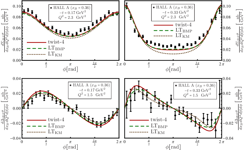
Figure 1: The unpolarized cross section [upper panels] and electron helicity dependent cross section difference [lower panels] from HALL A collaboration [12] vs. GK12 GPD model predictions.

As an example, we show in Fig. 1 [upper panels] the HALL A collaboration data [12] for the unpolarized cross section. Their description using popular GPD models is widely regarded as challenging. The data are compared with the QCD calculation using the GK12 GPD model in three different approximations: LT_KM (dotted curves), LT_BMP (dashed curves), and with the full account of kinematic twist-four effects (solid curves). The BH squared term is calculated using the formula set from [6]. Because of this contribution, the differences of the predictions of the unpolarized cross section in different models or approximations are washed out. Changing $\text{LT}_{\rm KM}\to\text{LT}_{\rm BMP}$ produces relative large enhancement of both the DVCS cross section and the interference term and the prediction becomes closer to the data, whereas the remaining kinematical twist corrections are hardly visible. Thus, for this observable, the $\text{LT}_{\rm BMP}$ approximation alone captures the main part of the total kinematic power correction.

The electron helicity dependent cross section difference is shown in Fig. 1 in the two lower panels. For $t=-0.33\,{\rm GeV}^{2}$ the differences in the three predictions are clearly visible and affect significantly the shape of the $\phi$-distribution. Having in mind the experimental errors, all of the predictions are, nevertheless, compatible with the data.

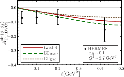
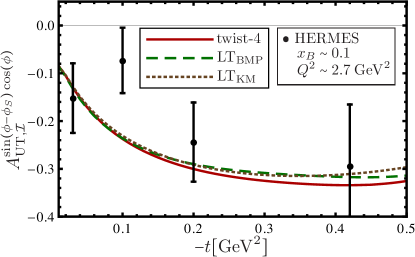
Figure 2: Transverse target spin asymmetries by HERMES collaboration [14].

The similar comparison for several DVCS observables for transversely polarized targets that are key to access the GPD $E$, is done in Ref. [13], see an example in Fig. 2. Surprisingly, we observe that also here the twist-corrections are rather mild. However, it is also known that the model dependence is rather strong [10].

To summarize, we have carried out a detailed numerical analysis of finite-$t$ and target mass corrections in DVCS, based on the recent calculation [1, 2, 3, 4] of the DVCS tensor to twist-four accuracy taking into account the descendants of the leading-twist operators. In order to discuss the impact of kinematic higher-twist corrections one has to formulate the LT approximation that would serve as the reference. This choice is not unique as the LT calculations are intrinsically ambiguous. In particular the change in the definition of the skewedness parameter has a large effect. It turns out that at least for some observables this difference presents the main source (numerically) of kinematic corrections, whereas the remaining higher-twist contributions to the BMP CFFs are rather mild. In future phenomenological studies it is highly advisable to implement besides the kinematical corrections also perturbative next-to-leading order corrections and, certainly, GPD evolution must be taken properly into account. This requires a change to global fitting routines that are based on appropriate GPD model parametrizations.

Acknowledgments:  This study was supported by the DFG, grant BR2021/5-2.

References

- [1] V. M. Braun and A. N. Manashov, Phys. Rev. Lett. 107 (2011) 202001.
- [2] V. M. Braun and A. N. Manashov, JHEP 1201 (2012) 085.
- [3] V. M. Braun, A. N. Manashov and B. Pirnay, Phys. Rev. D 86 (2012) 014003.
- [4] V. M. Braun, A. N. Manashov and B. Pirnay, Phys. Rev. Lett. 109 (2012) 242001.
- [5] V. M. Braun, A. N. Manashov, D. Müller and B. M. Pirnay, Phys. Rev. D 89 (2014) 074022.
- [6] A. V. Belitsky, D. Müller and A. Kirchner, Nucl. Phys. B 629 (2002) 323.
- [7] A. V. Belitsky and D. Müller, Phys. Rev. D 82 (2010) 074010.
- [8] A. V. Belitsky, D. Müller and Y. Ji, Nucl. Phys. B 878 (2014) 214.
- [9] K. Kumerički and D. Müller, Nucl. Phys. B 841 (2010) 1.
- [10] K. Kumerički, D. Müller and M. Murray, arXiv:1301.1230 [hep-ph].
- [11] P. Kroll, H. Moutarde and F. Sabatie, Eur. Phys. J. C 73 (2013) 2278.
- [12] C. M. Camacho et al. [Jefferson Lab Hall A Collaboration], Phys. Rev. Lett. 97 (2006) 262002.
- [13] B. Pirnay, Higher twist effects in deeply virtual Compton scattering, PhD Thesis (unpublished).
- [14] A. Airapetian et al. [HERMES Collaboration], JHEP 0806 (2008) 066.