Local properties of almost-Riemannian structures in dimension 3thanks: This research has been supported by the European Research Council, ERC StG 2009 “GeCoMethods”, contract number 239748 and by the Fondation Mathématique Jacques Hadamard.

U. Boscain G. Charlot M. Gaye P. Mason
Abstract

A 3D almost-Riemannian manifold is a generalized Riemannian manifold defined locally by 3 vector fields that play the role of an orthonormal frame, but could become collinear on some set $\mathcal{Z}$ called the singular set. Under the Hormander condition, a 3D almost-Riemannian structure still has a metric space structure, whose topology is compatible with the original topology of the manifold. Almost-Riemannian manifolds were deeply studied in dimension 2.

In this paper we start the study of the 3D case which appear to be reacher with respect to the 2D case, due to the presence of abnormal extremals which define a field of directions on the singular set. We study the type of singularities of the metric that could appear generically, we construct local normal forms and we study abnormal extremals. We then study the nilpotent approximation and the structure of the corresponding small spheres.

We finally give some preliminary results about heat diffusion on such manifolds.

Keywords: Almost-Riemannian structure, Sub-Riemannian geometry, cut locus, hypoelliptic diffusion  MSC: 53C17, 35H10

1 Introduction

A $n$-dimensional Almost Riemannian Structure ($n$-ARS for short) is a rank-varying sub-Riemannian structure that can be locally defined by a set of $n$ (and not by less than $n$) smooth vector fields on a $n$-dimensional manifold, satisfying the Hörmander condition (see for instance [2, 12, 31, 39]). These vector fields play the role of an orthonormal frame.

Let us denote by $\blacktriangle(q)$ the linear span of the vector fields at a point $q$. Around a point $q$ where $\blacktriangle(q)$ is $n$-dimensional, the corresponding metric is Riemannian.

On the singular set $\mathcal{Z}$, where $\blacktriangle(q)$ has dimension dim$(\blacktriangle(q))<n$, the corresponding Riemannian metric is not well-defined. However, thanks to the Hörmander condition, one can still define the Carnot–Caratheodory distance between two points, which happens to be finite and continuous.

Almost-Riemannian structures were deeply studied for $n=2$: they were introduced in the context of hypoelliptic operators [10, 27, 28]; they appeared in problems of population transfer in quantum systems [19, 20, 21] and have applications to orbital transfer in space mechanics [16, 15].

For 2-ARS, generically, the singular set is a $1$-dimensional embedded submanifold (see [7]) and there are three types of points: Riemannian points, Grushin points where $\blacktriangle(q)$ is $1$-dimensional and $\dim(\blacktriangle(q)+[\blacktriangle,\blacktriangle](q))=2$ and tangency points where $\dim(\blacktriangle(q)+[\blacktriangle,\blacktriangle](q))=1$ and the missing direction is obtained with one more bracket. Generically tangency points are isolated (see [7, 17]).

$2$-ARSs present very interesting phenomena. For instance, the presence of a singular set permits the conjugate locus to be nonempty even if the Gaussian curvature is negative where it is defined (see [7]). Moreover, a Gauss–Bonnet-type formula can be obtained [7, 23, 5].

In [18] a necessary and sufficient condition for two 2-ARSs on the same compact manifold $M$ to be Lipschitz equivalent was given. In [22] the heat and the Schrödinger equation with the Laplace–Beltrami operator on a 2-ARS were studied. In that paper it was proven that the singular set acts as a barrier for the heat flow and for a quantum particle, even though geodesics can pass through the singular set without singularities.

In this paper we start the study of 3-ARSs. An interesting feature of these structures is that abnormal extremals could be present. Abnormal extremals are special candidates to be length minimisers that cannot be obtained as a solution of Hamiltonian equations. They do not exist in Riemannian geometry and they could be present in sub-Riemannian geometry. Abnormal minimisers are responsible for the non sub-analyticity of the spheres in certain analytic cases [3] and they are the subject of one of the most important open question in sub-Riemannian geometry, namely “are length minimisers always smooth?” (see [6, 34]).

Moreover the presence of abnormal minimisers seems related to the non analytic hypoellipticity of the sub-Laplacian (built as the square of the vector fields defining the structure [25, 26, 38]).

The simplest example of analytic sub-Riemannian structure for which there are abnormal minimisers and for which the “sum of the square” is not analytic hypoelliptic is provided by a 3-ARS, namely the Baouendi-Goulaouic example, defined by the following three vector fields:

$\displaystyle X_{1}(x,y,z)=\left(\begin{array}[]{c}1\\ 0\\ 0\end{array}\right),~{}~{}~{}X_{2}(x,y,z)=\left(\begin{array}[]{c}0\\ 1\\ 0\end{array}\right),~{}~{}~{}X_{3}(x,y,z)=\left(\begin{array}[]{c}0\\ 0\\ x\end{array}\right).$ (10)

For this structure, the trajectory $(0,y_{0}+t,0)$ is an abnormal minimizer and the Green functions of the operator

$\displaystyle\partial_{t}\phi=\Delta\phi\mbox{ where }\Delta=X_{1}^{2}+X_{2}^{2}+X_{3}^{2}=\partial_{x}^{2}+\partial_{y}^{2}+x^{2}\partial_{z}^{2}$ (11)

are not analytic.

Our first result concerns the generic structure of singular sets for 3-ARSs. More precisely we prove that the following properties hold under generic conditions111 for the precise definition of generic see Definition 7

  • (G1)

    the dimension of $\blacktriangle(q)$ is larger than or equal to 2 and $\blacktriangle(q)+[\blacktriangle,\blacktriangle](q)=T_{q}M$, for every $q\in M$;

  • (G2)

    the singular set $\mathcal{Z}$ (i.e., the set of points where dim$(\mathcal{Z})<3$) is an embedded 2-dimensional manifold;

  • (G3)

    the points where $\blacktriangle(q)=T_{q}\mathcal{Z}$ are isolated.

As a consequence, under generic conditions, we can single out three types of points: Riemannian points (where dim$(\blacktriangle(q))=3$), type-1 points (where dim$(\blacktriangle(q))=2$ and $\blacktriangle(q)\neq T_{q}\mathcal{Z}$) and type-2 points (where $\blacktriangle(q)=T_{q}\mathcal{Z}$). See Figure 1. Moreover $\mathcal{Z}$ is formed by type-1 and type-2 points (type-2 points are isolated).

Refer to caption
$q$ ${\cal Z}$ $q$ $\blacktriangle(q)$ ${\cal Z}$ $\blacktriangle(q)$
Figure 1: The 3 type of points occurring in the generic case

Then for each type of point we build a local representation. See Theorem 2 below. These local representations are fundamental to study the local properties of the distance.

Next we study abnormal extremals. The intersection of $\blacktriangle$ with the tangent space to $\mathcal{Z}$ define a field of directions on $\mathcal{Z}$ whose integral trajectories are abnormal extremals. The singular points of this field of directions are type-2 points.

Since $\blacktriangle(q)+[\blacktriangle,\blacktriangle](q)=T_{q}M$ for every $q\in M$, as a consequence of a theorem of A.Agrachev and J.P. Gauthier [2, 8] if an abnormal extremal is optimal then it is not strict (i.e., it is at the same time a normal extremal). This condition is quite restrictive and indeed under generic conditions there are no abnormal minimisers.

We then focus on the nilpotent approximation of the structure at the different types of singular points. Obviously, at Riemannian points the nilpotent approximation is the Euclidean space. Interestingly, at type-1 points the nilpotent approximation depends on the point and it is a combination of an Heisenberg sub-Riemannian structure and a Baouendi-Goulaouic 3-ARS. Surprisingly the nilpotent approximation at a type-2 point is the Heisenberg sub-Riemannian structure and hence is not a 3-ARS.

We then describe the metric spheres for the nilpotent approximation for type-1 points. As explained above, type-1 points are the only ones for which the nilpotent approximation is not yet well understood. We recall that for small radii, sub-Riemannian balls tend to those of the nilpotent approximation (after a suitable rescaling) in the Hausdorff-Gromov sense.

We then study heat diffusion on 3-ARSs for nilpotent structures of type-1. We study the diffusion related to two types of operators: $\Delta_{L}$, the Laplace operator built as the divergence of the horizontal gradient, where the divergence is computed with respect to the Euclidean volume and $\Delta_{\omega}$, the Laplace operator built in the same way, but with the divergence computed with respect to the intrinsic (diverging on $\mathcal{Z}$) Riemannian volume. The first operator is hypoelliptic and for it we compute the explicit expression of the heat kernel. For the second operator we prove that it is not hypoelliptic and that the singular set $\mathcal{Z}$ acts as a barrier for the heat flow.

Structure of the paper. Section 2 contains generalities about ARS. Section 3 contains the construction (under generic conditions) of the local representations. Section 4 contains results on abnormal extremals. Section 5 contains the analysis of the spheres and of the cut locus for the nilpotent points of type-1. This is the most important and technical part of the paper. Section 6 contains the discussion of the heat diffusion on 3-ARS. Appendix A contains the proof of the genericity of (G1), (G2), (G3). Appendix B contains the explicit construction of the heat kernel for $\Delta_{L}$.

2 Basic Definitions

Definition 1

A $n$-dimensional almost-Riemannian structure ($n$-ARS, for short) is a triple ${\mathcal{S}}=(E,\mathfrak{f},\langle\cdot,\cdot\rangle)$ where $E$ is a vector bundle of rank $n$ over a $n$ dimensional smooth manifold $M$ and $\langle\cdot,\cdot\rangle$ is a Euclidean structure on $E$, that is, $\langle\cdot,\cdot\rangle_{q}$ is a scalar product on $E_{q}$ smoothly depending on $q$. Finally $\mathfrak{f}:E\rightarrow TM$ is a morphism of vector bundles, i.e., (i) the diagram

(16)

commutes, where $\pi:TM\rightarrow M$ and $\pi_{E}:E\rightarrow M$ denote the canonical projections and (ii) $\mathfrak{f}$ is linear on fibers.

Denoting by $\Gamma(E)$ the $C^{\infty}(M)$-module of smooth sections on $E$, and by $\mathfrak{f}_{*}:\Gamma(E)\rightarrow\mathrm{Vec}(M)$ the map $\sigma\mapsto\mathfrak{f}_{*}(\sigma):=\mathfrak{f}\circ\sigma$, we require that the submodule of Vec$(M)$ given by $\blacktriangle=\mathfrak{f}_{*}(\Gamma(E))$ to be bracket generating, i.e., $Lie_{q}(\blacktriangle)=T_{q}M$ for every $q\in M$. Moreover, we require that $\mathfrak{f}_{*}$ is injective.

Here Lie$(\blacktriangle)$ is the smallest Lie subalgebra of Vec(M) containing $\blacktriangle$ and Lie${}_{q}(\blacktriangle)$ is the linear subspace of $T_{q}M$ whose elements are evaluation at $q$ of elements belonging to Lie$(\blacktriangle)$. The condition that $\blacktriangle$ satisfies the Lie bracket generating assumption is also known as the Hörmander condition.

We say that a $n$-ARS $(E,\mathfrak{f},\langle\cdot,\cdot\rangle)$ is trivializable if $E$ is isomorphic to the trivial bundle $M\times\mathbb{R}^{n}$. A particular case of $n$-ARSs is given by $n$-dimensional Riemannian manifolds. In this case $E=TM$ and $\mathfrak{f}$ is the identity.

Let ${\mathcal{S}}=(E,\mathfrak{f},\langle\cdot,\cdot\rangle)$ be a $n$-ARS on a manifold $M$. We denote by $\blacktriangle(q)$ the linear subspace $\{V(q)\mid V\in\blacktriangle\}=\mathfrak{f}(E_{q})\subseteq T_{q}M$. The set of points in $M$ such that $\dim(\blacktriangle(q))<n$ is called singular set and denoted by $\mathcal{Z}$.

If $(\sigma_{1},\ldots,\sigma_{n})$ is an orthonormal frame for $\langle\cdot,\cdot\rangle$ on an open subset $\Omega$ of $M$, an orthonormal frame on $\Omega$ is given by $(\mathfrak{f}\circ\sigma_{1},\ldots,\mathfrak{f}\circ\sigma_{n})$. Orthonormal frames are systems of local generators of $\blacktriangle$.

For every $q\in M$ and every $v\in\blacktriangle(q)$ define

$${{\bf G}}_{q}(v)=\min\{\langle u,u\rangle_{q}\mid u\in E_{q},\mathfrak{f}(u)=v\}.$$

For a vector field $X$, we call $\sqrt{{{\bf G}}_{q}(X(q))}$ the ponctual norm of $X$ at $q$.

An absolutely continuous curve $\gamma:[0,T]\to M$ is admissible for ${\mathcal{S}}$ if there exists a measurable essentially bounded function

$$[0,T]\ni t\mapsto u(t)\in E_{\gamma(t)},$$

called control function such that $\dot{\gamma}(t)=\mathfrak{f}(u(t))$ for almost every $t\in[0,T]$. Given an admissible curve $\gamma:[0,T]\to M$, the length of $\gamma$ is

$\displaystyle\ell(\gamma)=\int_{0}^{T}\sqrt{{\bf G}_{\gamma(t)}(\dot{\gamma}(t))}~{}dt.$

The Carnot-Caratheodory distance (or sub-Riemannian distance) on $M$ associated with ${\mathcal{S}}$ is defined as

$\displaystyle d(q_{0},q_{1})=\inf\{\ell(\gamma)\mid\gamma(0)=q_{0},\gamma(T)=q_{1},\gamma\ \mathrm{admissible}\}.$

It is a standard fact that $\ell(\gamma)$ is invariant under reparameterization of the curve $\gamma$. Moreover, if an admissible curve $\gamma$ minimizes the so-called energy functional $E(\gamma)=\int_{0}^{T}{\bf G}_{\gamma(t)}(\dot{\gamma}(t))~{}dt$ with $T$ fixed (and fixed initial and final point) then $v(t)=\sqrt{{\bf G}_{\gamma(t)}(\dot{\gamma}(t))}$ is constant and $\gamma$ is also a minimizer of $\ell(\cdot)$. On the other hand, a minimizer $\gamma$ of $\ell(\cdot)$, such that $v$ is constant, is a minimizer of $E(\cdot)$ with $T=\ell(\gamma)/v$.

The finiteness and the continuity of $d(\cdot,\cdot)$ with respect to the topology of $M$ are guaranteed by the Lie bracket generating assumption on the $n$-ARS (see [9]). The Carnot-Caratheodory distance endows $M$ with the structure of metric space compatible with the topology of $M$ as differential manifold.

When the $n$-ARS is trivializable, the problem of finding a curve minimizing the energy between two fixed points $q_{0},q_{1}\in M$ is naturally formulated as the distributional optimal control problem with quadratic cost and fixed final time

$\displaystyle\dot{q}=\sum_{i=1}^{n}u_{i}X_{i}(q)\,,~{}~{}u_{i}\in\mathbb{R}\,,~{}~{}\int_{0}^{T}\sum_{i=1}^{n}u_{i}^{2}(t)~{}dt\to\min,~{}~{}q(0)=q_{0},~{}~{}q(T)=q_{1}.$ (17)

where $\{X_{1},\ldots,X_{n}\}$ is an orthonormal frame.

2.1 Minimizers and geodesics

In this section we briefly recall some facts about geodesics in $n$-ARSs. In particular, we define the corresponding exponential map.

Definition 2

A geodesic for a $n$-ARS is an admissible curve $\gamma:[0,T]\to M$ such that ${\bf G}_{\gamma(\cdot)}(\dot{\gamma}(\cdot))$ is constant and, for every sufficiently small interval $[t_{1},t_{2}]\subset[0,T]$, the restriction $\gamma_{|_{[t_{1},t_{2}]}}$ is a minimizer of $\ell(\cdot)$. A geodesic for which ${\bf G}_{\gamma(\cdot)}(\dot{\gamma}(\cdot))=1$ is said to be parameterized by arclength.

A $n$-ARS is said to be complete if $(M,d)$ is complete as a metric space. If the sub-Riemannian metric is the restriction of a complete Riemannian metric, then it is complete.

Under the assumption that the manifold is complete, a version of the Hopf-Rinow theorem (see [24, Chapter 2]) implies that the manifold is geodesically complete (i.e. all geodesics are defined for every $t\geq 0$) and that for every two points there exists a minimizing geodesic connecting them.

Trajectories minimizing the distance between two points are solutions of first order necessary conditions for optimality, which in the case of sub-Riemannian geometry are given by a weak version of the Pontryagin Maximum Principle ([35]).

Theorem 1

Let $q(\cdot)$ be a solution of the minimization problem (17) such that ${\bf G}_{q(\cdot)}(\dot{q}(\cdot))$ is constant and $u(\cdot)$ be the corresponding control. Then there exists a Lipschitz map $p:t\in[0,T]\mapsto p(t)\in T^{*}_{q(t)}M\setminus\{0\}$ such that one and only one of the following conditions holds:

  • (i)

    $\dot{q}=\dfrac{\partial H}{\partial p},\quad\dot{p}=-\dfrac{\partial H}{\partial q},\quad u_{i}(t)=\left\langle p(t),X_{i}(q(t))\right\rangle,$ where $H(q,p)=\frac{1}{2}\sum_{i=1}^{n}\left\langle p,X_{i}(q)\right\rangle^{2}$.

  • (ii)

    $\dot{q}=\dfrac{\partial{\cal H}}{\partial p},\quad\dot{p}=-\dfrac{\partial{\cal H}}{\partial q},\quad 0=\left\langle p(t),X_{i}(q(t))\right\rangle,$ where ${\cal H}(t,q,p)=\sum_{i=1}^{n}u_{i}(t)\left\langle p,X_{i}(q)\right\rangle$.

For an elementary proof of Theorem 1 see [2].

Remark 1

If $(q(\cdot),p(\cdot))$ is a solution of (i) (resp. (ii)) then it is called a normal extremal (resp. abnormal extremal). It is well known that if $(q(\cdot),p(\cdot))$ is a normal extremal then $q(\cdot)$ is a geodesic (see [2]). This does not hold in general for abnormal extremals. An admissible trajectory $q(\cdot)$ can be at the same time normal and abnormal (corresponding to different covectors). If an admissible trajectory $q(\cdot)$ is normal but not abnormal, we say that it is strictly normal. An abnormal extremal such that $q(\cdot)$ is constant, is called trivial.

In the following we denote by $(q(t),p(t))=e^{t\vec{H}}(q_{0},p_{0})$ the solution of $(i)$ with initial condition $(q(0),p(0))=(q_{0},p_{0})$. Moreover we denote by $\pi:T^{*}M\to M$ the canonical projection.

Normal extremals (starting from $q_{0}$) parametrized by arclength correspond to initial covectors $p_{0}\in\Lambda_{q_{0}}:=\{p_{0}\in T^{*}_{q_{0}}M|\,H(q_{0},p_{0})=1/2\}.$

Definition 3

Consider a $n$-ARS. We define the exponential map starting from $q_{0}\in M$ as

$\displaystyle\mathcal{E}_{q_{0}}:\Lambda_{q_{0}}\times\mathbb{R}^{+}\to M,\qquad\mathcal{E}_{q_{0}}(p_{0},t)=\pi(e^{t\vec{H}}(q_{0},p_{0})).$ (18)

Notice that each $\mathcal{E}_{q_{0}}(p_{0},\cdot)$ is a geodesic. Next, we recall the definition of cut and conjugate time.

Definition 4

Let $q_{0}\in M$ and $\gamma(t)$ an arclength geodesic starting from $q_{0}$. The cut time for $\gamma$ is $t_{cut}(\gamma)=\sup\{t>0,\,\gamma|_{[0,t]}\text{ is optimal}\}$. The cut locus from $q_{0}$ is the set $\operatorname{Cut}(q_{0})=\{\gamma(t_{cut}(\gamma)),\gamma$ arclength geodesic from $q_{0}\}$.

Definition 5

Let $q_{0}\in M$ and $\gamma(\cdot)=\mathcal{E}_{q_{0}}(p_{0},\cdot)$, $p_{0}\in\Lambda_{q_{0}}$ a normal arclength geodesic. The first conjugate time of $\gamma$ is $t_{con}(\gamma)=\min\{t>0,\ (p_{0},t)$ is a critical point of $\mathcal{E}_{q_{0}}\}$. The first conjugate locus from $q_{0}$ is the set $\operatorname{Con}(q_{0})=\{\gamma(t_{con}(\gamma)),\gamma$ normal arclength geodesic from $q_{0}\}$.

It is well known that, for a geodesic $\gamma$ which is not abnormal, the cut time $t_{*}=t_{cut}(\gamma)$ is either equal to the conjugate time or there exists another geodesic $\widetilde{\gamma}$ such that $\gamma(t_{*})=\widetilde{\gamma}(t_{*})$ (see for instance [4]).

Let $(q(\cdot),p(\cdot))$ be an abnormal extremal. In the following we use the convention that all points of Supp$(q(\cdot))$ are conjugate points.

Remark 2

In $n$-ARSs, the exponential map starting from $q_{0}\in\mathcal{Z}$ is never a local diffeomorphism in a neighborhood of the point $q_{0}$ itself. As a consequence the metric balls centered in $q_{0}$ are never smooth and both the cut and the conjugate loci from $q_{0}$ are adjacent to the point $q_{0}$ itself (see [1]).

To study local properties of $n$-ARSs, it is useful to use local representations.

Definition 6

A local representation of a $n$-ARS ${\mathcal{S}}$ at a point $q\in M$ is a $n$-tuple of vector fields $(X_{1},\ldots,X_{n})$ on $\mathbb{R}^{n}$ such that there exist: i) a neighborhood $U$ of $q$ in $M$, a neighborhood $V$ of the origin in $\mathbb{R}^{n}$ and a diffeomorphism $\varphi:U\rightarrow V$ such that $\varphi(q)=(0,\ldots,0)$; ii) a local orthonormal frame $(F_{1},\dots,F_{n})$ of ${\mathcal{S}}$ around $q$, such that $\varphi_{*}F_{1}=X_{1}$, $\varphi_{*}F_{2}=X_{2},\ldots,\varphi_{*}F_{n}=X_{n}$ where $\varphi_{*}$ denotes the push-forward.

3 Local Representations

The main purpose of this section is to give local representations of 3-ARS under generic conditions.

Definition 7

A property $(P)$ defined for 3-ARSs is said to be generic if for every rank-3 vector bundle $E$ over $M$, $(P)$ holds for every $\mathfrak{f}$ in a residual subset of the set of morphisms of vector bundles from $E$ to $TM$, endowed with the ${\mathcal{C}}^{\infty}$-Whitney topology, such that $(M,E,\mathfrak{f})$ is a 3-ARS.

For the definition of residual subset, see Appendix A. We have the following

Proposition 1

Consider a 3-ARS. The following conditions are generic for 3-ARSs.

(G1) dim($\blacktriangle(q))\geq 2$ and $\blacktriangle(q)+[\blacktriangle,\blacktriangle](q)=T_{q}M$ for every $q\in M$;

(G2) $\mathcal{Z}$ is an embedded two-dimensional submanifold of $M$;

(G3) the points where $\blacktriangle(q)=T_{q}\mathcal{Z}$ are isolated.

For the proof see Appendix A. In the following we refer to the set of conditions (G1), (G2), (G3) as to the (G) condition. (G) is the condition under which the main results of the paper are proved.

A way of rephrasing Proposition 1 is the following (see Figure 1):
Proposition 1bis Under the condition (G) on the 3-ARS there are three types of points:

  • Riemannian points where $\blacktriangle(q)=T_{q}M$.

  • type-1 points where $\blacktriangle(q)$ has dimension 2 and is transversal to $\mathcal{Z}$.

  • type-2 points where $\blacktriangle(q)$ has dimension 2 and is tangent to $\mathcal{Z}$.

Moreover type-2 points are isolated, type-1 points form a 2 dimensional manifold and all the other points are Riemannian points.
The main result of this section is the following Theorem.

Theorem 2

If a 3-ARS satisfies (G) then for every point $q\in M$ there exists a local representation having the form

$\displaystyle X_{1}(x,y,z)=\left(\begin{array}[]{c}1\\ 0\\ 0\end{array}\right),~{}~{}~{}X_{2}(x,y,z)=\left(\begin{array}[]{c}0\\ \alpha(x,y,z)\\ \beta(x,y,z)\end{array}\right),~{}~{}~{}X_{3}(x,y,z)=\left(\begin{array}[]{c}0\\ 0\\ \nu(x,y,z)\end{array}\right),~{}~{}~{}$ (28)

where $\alpha(0,0,0)=1$, $\beta(0,0,0)=0$. Moreover one of following conditions holds:

Riemannian case:

$\nu(0,0,0)=1$.

type-1 case:

$\alpha=1+x\bar{\alpha}$, $\beta=x\bar{\beta}$, $\nu=x\bar{\nu}$ where $\bar{\alpha}$, $\bar{\beta}$, $\bar{\nu}$ are smooth functions such that $\bar{\nu}(0,0,z)^{2}+\bar{\beta}(0,0,z)^{2}=1$. Moreover the function $\bar{\nu}$ may have zeros only on the plane $\{x=0\}$.

type-2 case:

$\alpha=1+x\bar{\alpha}_{1}+h\bar{\alpha}_{2}$, $\beta=x\bar{\beta}_{1}+h\bar{\beta}_{2}$ and $\nu=h\bar{\nu}$ where $\bar{\nu}$, $\bar{\alpha}_{i}$ and $\bar{\beta}_{i}$, $i=1,2$ are smooth functions such that $\bar{\beta}_{1}(0,0,0)\neq 0$, $h(x,y,z)=z-\varphi(x,y)$ with $\varphi$ a smooth function satisfying $\varphi(0,0)=\frac{\partial\varphi}{\partial x}(0,0)=\frac{\partial\varphi}{\partial y}(0,0)=\frac{\partial^{2}\varphi}{\partial x\partial y}(0,0)=0$. Moreover the function $\bar{\nu}$ may have zero only on $\{h(x,y,z)=0\}$ which defines a two-dimensional surface.

Remark 3

Notice that Theorem 2 implies that

  • in the type-1 case, $\mathcal{Z}=\{x=0\}$.

  • in the type-2 case, the set $\mathcal{Z}=\{h(x,y,z)=0\}$ has its tangent space at zero equal to span$\{\partial_{x},\partial_{y}\}$. Moreover, the set of type-2 points being discrete, we can assume the generic condition

    (iiibis) $\bar{\nu}(0,0,0)\neq 0$, $\frac{\partial^{2}\varphi}{\partial x^{2}}(0,0)\neq 0$ and $\frac{\partial^{2}\varphi}{\partial y^{2}}(0,0)\neq 0$.

    Condition (iiibis) implies that in the type-2 case $\nu=az+bx^{2}+cy^{2}+o(x^{2}+y^{2}+|z|)$ where $a$, $b$ and $c$ are not zero.

Remark 4

Notice that in a neighbourhood where the almost-Riemannian structure is expressed in the form (28) the corresponding Riemannian metric has the expression (where it is defined)

$$\left(\begin{array}[]{ccc}1&0&0\\ 0&\frac{\beta^{2}+\nu^{2}}{\alpha^{2}\nu^{2}}&-\frac{\beta}{\alpha\nu^{2}}\\ 0&-\frac{\beta}{\alpha\nu^{2}}&\frac{1}{\nu^{2}}\\ \end{array}\right).$$

The corresponding Riemannian volume is (where it is defined)

$\displaystyle\omega(x)=\frac{1}{\sqrt{\alpha(x)^{2}\nu(x)^{2}}}dx\wedge dy\wedge dz$ (29)

3.1 Proof of Theorem 2

Let $W$ be a 2-dimensional surface transversal to ${\blacktriangle}$ at $q$.

Lemma 1

There exist a local coordinate system $(x,y,z)$ centered at $q$ such that $W=\{x=0\}$, $t\mapsto(t,y,z)$ is a geodesic transversal to $W$ for every $(y,z)$ and the following triple is an orthonormal frame of the metric

$$X_{1}(x,y,z)=\left(\begin{array}[]{c}1\\ 0\\ 0\end{array}\right),~{}~{}~{}X_{2}(x,y,z)=\left(\begin{array}[]{c}0\\ \alpha(x,y,z)\\ \beta(x,y,z)\end{array}\right),~{}~{}~{}X_{3}(x,y,z)=\left(\begin{array}[]{c}0\\ 0\\ \nu(x,y,z)\end{array}\right),~{}~{}~{}$$

where $\alpha$, $\beta$ and $\nu$ are smooth functions with $\alpha(0,0,0)\neq 0$.

Proof Assume that a coordinate system $(y,z)$ is fixed on $W$ and fix a transversal orientation along $W$. Then consider the family of geodesics $t\mapsto\gamma_{yz}(t)$ parameterized by arclength, positively oriented and transversal to $W$ at $(y,z)$. The map $(x,y,z)\mapsto\gamma_{yz}(x)$ is a local diffeomorphism and hence defines a coordinate system. In this system $\partial_{x}(q)$ has norm 1 and is orthogonal, with respect to ${\bf G}_{q}$, to $T_{q}\{x=c\}\cap\blacktriangle_{q}$ for any constant $c$ close to 0. Call it $X_{1}^{\prime}$.

Now, since the distribution has dimension at least two at each point, one can find a vector field $X_{2}^{\prime}$ of the distribution of norm one whose ponctual norm is equal to 1 and which is orthogonal to $X_{1}^{\prime}$. It is tangent to ${x=c}$ for any constant $c$ close to 0. We can fix the coordinate system on $W$ in such a way $X_{2}^{\prime}(0,y,z)=\partial_{y}(0,y,z)$. If we complete the orthonormal frame with a vector field $X_{3}^{\prime}$ we find that

$$X_{1}^{\prime}(x,y,z)=\left(\begin{array}[]{c}1\\ 0\\ 0\end{array}\right),~{}~{}~{}X_{2}^{\prime}(x,y,z)=\left(\begin{array}[]{c}0\\ \alpha_{1}(x,y,z)\\ \beta_{1}(x,y,z)\end{array}\right),~{}~{}~{}X_{3}^{\prime}(x,y,z)=\left(\begin{array}[]{c}0\\ \mu_{1}(x,y,z)\\ \nu_{1}(x,y,z)\end{array}\right),$$

with $\alpha_{1}(0,y,z)=1$ and $\beta_{1}(0,y,z)=0$. Locally $\alpha_{1}^{2}(0,0,0)+\mu_{1}^{2}(0,0,0)>0$ hence we can choose the orthonormal frame $(X_{1},X_{2},X_{3})=(X_{1}^{\prime},\frac{\alpha_{1}X_{2}^{\prime}+\mu_{1}X_{3}^{\prime}}{\sqrt{\alpha_{1}^{2}+\mu_{1}^{2}}},\frac{-\mu_{1}X_{2}^{\prime}+\alpha_{1}X_{3}^{\prime}}{\sqrt{\alpha_{1}^{2}+\mu_{1}^{2}}})$ satisfying

$$X_{1}(x,y,z)=\left(\begin{array}[]{c}1\\ 0\\ 0\end{array}\right),~{}~{}~{}X_{2}(x,y,z)=\left(\begin{array}[]{c}0\\ \alpha(x,y,z)\\ \beta(x,y,z)\end{array}\right),~{}~{}~{}X_{3}(x,y,z)=\left(\begin{array}[]{c}0\\ 0\\ \nu(x,y,z)\end{array}\right),$$

where $\alpha=\sqrt{\alpha_{1}^{2}+\mu_{1}^{2}}$, $\beta=\frac{\alpha_{1}\beta_{1}+\mu_{1}\nu_{1}}{\sqrt{\alpha_{1}^{2}+\mu_{1}^{2}}}$ and $\nu=\frac{-\mu_{1}\beta_{1}+\alpha_{1}\nu_{1}}{\sqrt{\alpha_{1}^{2}+\mu_{1}^{2}}}$. $\blacksquare$


End of the proof of Theorem 2: Let us start with the Riemannian case. In the construction, we are still free in fixing the vertical axis, that is the curve $z\mapsto(0,0,z)$. Let us choose it orthogonal to $X_{2}$ and parameterized such that $\partial_{z}(0,0,z)$ has norm one. Then $\mu_{1}(0,0,z)=0$ and $\nu_{1}(0,0,z)=1$ for $z$ small enough. As a consequence, since $\alpha_{1}(0,0,0)=1$ and $\beta_{1}(0,0,0)=0$ we find at $(0,0,0)$

$$X_{2}=\left(\begin{array}[]{c}0\\ \sqrt{\alpha_{1}^{2}+\mu_{1}^{2}}\\ \frac{\alpha_{1}\beta_{1}+\mu_{1}\nu_{1}}{\sqrt{\alpha_{1}^{2}+\mu_{1}^{2}}}\end{array}\right)=\left(\begin{array}[]{c}0\\ 1\\ 0\end{array}\right),~{}~{}~{}X_{3}=\left(\begin{array}[]{c}0\\ 0\\ \frac{-\mu_{1}\beta_{1}+\alpha_{1}\nu_{1}}{\sqrt{\alpha_{1}^{2}+\mu_{1}^{2}}}\end{array}\right)=\left(\begin{array}[]{c}0\\ 0\\ 1\end{array}\right),$$

which finishes the proof for the Riemannian case.

Let us assume now that $q\in\mathcal{Z}$. Since in the construction in the proof of lemma 1 $X_{1}$ and $X_{2}$ are assumed of ponctual norm 1, then $X_{3}$ is zero along $\mathcal{Z}$. hence $\mu=\nu=0$ on $\mathcal{Z}$. Hence

$$X_{2}=\left(\begin{array}[]{c}0\\ \alpha\\ \beta\end{array}\right),~{}~{}~{}X_{3}=\left(\begin{array}[]{c}0\\ 0\\ \nu\end{array}\right),$$

where $\alpha=\alpha_{1}$, $\beta=\beta_{1}$ and $\nu=0$ on $\mathcal{Z}$.

Now, if $\mathcal{Z}$ is transversal to the distribution, one can fix $W=\mathcal{Z}=\{x=0\}$ which implies that $\alpha=1$ and $\beta=0$ for $x=0$ since $W=\{x=0\}$, and $\nu=0$ for $x=0$ since $\mathcal{Z}=\{x=0\}$. As a consequence $\alpha=1+x\bar{\alpha}$, $\beta=x\bar{\beta}$, $\nu=x\bar{\nu}$ where $\bar{\alpha}$, $\bar{\beta}$, $\bar{\nu}$ are smooth functions. The fact that $[{\blacktriangle},{\blacktriangle}](q)=T_{q}M$ implies that $\bar{\beta}(0,0,0)\neq 0$ or $\bar{\nu}(0,0,0)\neq 0$. Up to a reparameterization of the $z$-axis, one can hence assume that $\bar{\beta}(0,0,z)^{2}+\bar{\nu}(0,0,z)^{2}=1$ for $z$ small enough.

Finally, if $\mathcal{Z}$ is tangent to the distribution then its tangent space at $q$ is generated by $X_{1}(q)$ and $X_{2}(q)$. This implies that it exists $\varphi$ sur that $\mathcal{Z}=\{h(x,y,z)=z-\varphi(x,y)=0\}$ where $\varphi$ is a smooth function such that $\varphi(0,0)=\frac{\partial\varphi}{\partial x}(0,0)=\frac{\partial\varphi}{\partial y}(0,0)=0$. Now, up to a rotation in the $(x,y)$-coordinates (and in the choice of $X_{1}$ and $X_{2}$) we can moreover assume that $\frac{\partial^{2}\varphi}{\partial x\partial y}(0,0)=0$. The fact that $\bar{\nu}$ has no zero outside $\{h(x,y,z)=0\}$ is a consequence of the fact that this last set is a two dimensional manifold passing through $q$ which is included in $\mathcal{Z}$ implying that locally $\mathcal{Z}=\{h(x,y,z)=0\}$.

4 Abnormal extremals

In this section we investigate the presence and characterization of abnormal extremals for 3-ARS. Notice that, on one hand, there are no abnormal extremals starting from a Riemannian point. On the other hand, as we will see, from type-1 points abnormal extremals start, except in some exceptional case. Roughly speaking, abnormal extremals can be described as trajectories of a field of directions defined on the surface $\mathcal{Z}$ and corresponding, at a given point $q$ of $\mathcal{Z}$, to the one-dimensional intersection $T_{q}\mathcal{Z}\cap\blacktriangle(q)$. Let us formalize this point.

Assume that (G) holds. Let $q_{0}\in\mathcal{Z}$ be of type-1 and assume that $X_{1},X_{2},X_{3}$ are vector fields spanning $\blacktriangle$ in a neighborhood of $q_{0}$ such that $X_{1}(q_{0})\wedge X_{2}(q_{0})\neq 0$. Assume moreover that $\sum_{i=1}^{3}\det\left(X_{1}(q_{0}),X_{2}(q_{0}),[X_{i-1},X_{i+1}](q_{0})\right)X_{i}(q_{0})\neq 0$, with the convention that $X_{0}=X_{3},\ X_{4}=X_{1}$. This condition is satisfied in the whole $\mathcal{Z}$ except some isolated points. Then we claim that there exists an open neighborhood $U$ of $q_{0}$ such that for any point $q\in U\cap\mathcal{Z}$ there exists only one nontrivial abnormal extremal passing through $q$ and the latter is, up to reparametrization, a trajectory of the vector field

$\displaystyle X(q)=\sum_{i=1}^{3}u_{i}(q)X_{i}(q)$ (30)
$\displaystyle u_{i}(q)=\det\left(X_{1}(q),X_{2}(q),[X_{i-1},X_{i+1}](q)\right),\quad i=1,2,3.$ (31)

From the Pontryagin maximum principle we have that with each abnormal extremal $q(\cdot)$ one can associate an adjoint vector $p(\cdot)$ such that $\langle p(t),X_{i}(q(t))\rangle=0$, for $i=1,2,3$. It turns out that $q(\cdot)$ must be contained in $\mathcal{Z}$ and, in a neighborhood of $q_{0}$, $p(t)$ must be proportional to the nonzero vector $X_{1}(q(t))\wedge X_{2}(q(t))$. By differentiating with respect to time the equality $\langle p(t),X_{i}(q(t))\rangle=0$, and knowing that the adjoint vector $p$ satisfies the equation

$$\dot{p}=\sum_{i=1}^{3}u_{i}\left(\frac{\partial X_{i}}{dq}\right)^{T}p$$

we get that $\sum_{j\neq i}u_{j}\langle p,[X_{i},X_{j}]\rangle=0$ leading to

$$\sum_{j\neq i}u_{j}\langle X_{1}\wedge X_{2},[X_{i},X_{j}]\rangle=\sum_{j\neq i}u_{j}\,\det(X_{1},X_{2},[X_{i},X_{j}])=0.$$

Whenever the triple of components $\mathrm{det}(X_{1},X_{2},[X_{i},X_{j}])$, $i\neq j$ is different from 00 we get that the linear equation above is satisfied for the $u_{i}$’s given in (31). Taking into account the local representation given in Theorem 2 one can see by a direct computation, and by using the fact that $\partial_{x}\beta(0,0,0)\neq 0$ or $\partial_{x}\nu(0,0,0)\neq 0$, that such a triple is always nonzero for a type-1 point. Note that the condition $X(0)\neq 0$ characterizing the possibility of having a nontrivial abnormal extremal parameterized by arclength passing through the origin is verified whenever $\bar{\nu}(0,0,0)\neq 0$. Note also that, close to a type-1 point, the equations $\langle p,X_{i}(q)\rangle=0,\ i=1,2,3,$ define a three-dimensional submanifold of $T^{*}M$ (this can be checked easily via the local representation of $X_{1},X_{2},X_{3}$). The Hamiltonian field, with $u_{i}=u_{i}(q)$, turns out to be tangent to such submanifold, confirming that the abnormal extremals are exactly those trajectories that satisfy (30)-(31).

On a type-2 point, again by direct computation with the local representation defined as in Theorem 2, one sees that the vector field $X$ vanishes at $q_{0}=0$. By considering $x,y$ as local coordinates in $\mathcal{Z}$, we have the following linearized equation for the abnormal extremals around the type-2 point

$\displaystyle\dot{x}$ $\displaystyle=$ $\displaystyle 2by-x\bar{\beta}_{1}(0,0,0)$
$\displaystyle\dot{y}$ $\displaystyle=$ $\displaystyle-2ax$

where $a=\frac{\partial^{2}\varphi}{\partial x^{2}}$ and $b=\frac{\partial^{2}\varphi}{\partial y^{2}}$. Note that, depending on the values $a,b,\bar{\beta}_{1}(0,0,0)$, the previous system can be stable or unstable, and may have real or complex non-real eigenvalues. Moreover, since $u_{1}(0)=-\bar{\beta}_{1}(0,0,0)\neq 0$, it turns out that abnormal extremals parameterized by arclength cannot reach or escape from a type-2 point in finite time.

Concerning optimality of abnormal extremals, since $\blacktriangle(q)+[\blacktriangle,\blacktriangle](q)=T_{q}M$ for every $q\in M$, as a consequence of a Theorem of A.Agrachev and J.P. Gauthier [2, 8] if an abnormal extremal is optimal then it is not strict. Generically this can never happen. Let us notice that, since the vector field $X_{3}$ is zero on $\mathcal{Z}$ with respect to the chosen local representation, optimality would imply that $u_{3}=0$ locally along the trajectory, and this implies $\partial_{x}\beta=\bar{\beta}=0$ along the trajectory.

Refer to caption
type-2 points$\mathcal{Z}$
Figure 2: The singular set $\mathcal{Z}$ with the field of abnormal extremals. The type-2 points correspond to to singularity of this field. All other points on $\mathcal{Z}$ are type-1 points.

The following theorem summarizes the results obtained in this section.

Theorem 3

For any type-1 point there exists an abnormal extremal, parameterized by arclength passing through it if and only if

$$\sum_{i=1}^{3}\det\left(X_{1}(q_{0}),X_{2}(q_{0}),[X_{i-1},X_{i+1}](q_{0})\right)X_{i}(q_{0})\neq 0,$$

with the convention that $X_{0}=X_{3},\ X_{4}=X_{1}$. Using the local representation given by Theorem 2, this condition is equivalent to $\bar{\nu}(0,0,0)\neq 0$. There is no nontrivial abnormal extremal passing through type-2 points, which are poles of the extremal flow corresponding to abnormal extremals.

Generically all nontrivial abnormal extremals are not optimal and they are strictly abnormal.

Remark 5

If $q_{0}$ is a type-1 point such that $\sum_{i=1}^{3}\det\left(X_{1}(q_{0}),X_{2}(q_{0}),[X_{i-1},X_{i+1}](q_{0})\right)X_{i}(q_{0})=0,$ then the trajectory $q(\cdot)=q_{0}$ is a trivial abnormal extremal.

5 Nilpotent approximations

For each kind of points it is an easy exercise to find the nilpotent approximation in the coordinate system constructed in the local representation. For the general theory of the nilpotent approximation, see, for instance, [2, 12]. We have:

  • in the Riemannian case

    $$\hat{X}_{1}(x,y,z)=\left(\begin{array}[]{c}1\\ 0\\ 0\end{array}\right),~{}~{}~{}\hat{X}_{2}(x,y,z)=\left(\begin{array}[]{c}0\\ 1\\ 0\end{array}\right),~{}~{}~{}\hat{X}_{3}(x,y,z)=\left(\begin{array}[]{c}0\\ 0\\ 1\end{array}\right),$$
  • in the type-1 case

    X^1(x,y,z)=(100),X^2(x,y,z)=(01cos(σ)x),X^3(x,y,z)=(00sin(σ)x),formulae-sequencesubscript^𝑋1𝑥𝑦𝑧100formulae-sequencesubscript^𝑋2𝑥𝑦𝑧01𝜎𝑥subscript^𝑋3𝑥𝑦𝑧00𝜎𝑥\hat{X}_{1}(x,y,z)=\left(\begin{array}[]{c}1\\ 0\\ 0\end{array}\right),~{}~{}~{}\hat{X}_{2}(x,y,z)=\left(\begin{array}[]{c}0\\ 1\\ \cos(\sigma)x\end{array}\right),~{}~{}~{}\hat{X}_{3}(x,y,z)=\left(\begin{array}[]{c}0\\ 0\\ \sin(\sigma)x\end{array}\right),

    where $\sigma\in[0,\pi/2]$ is a parameter.

  • in the type-2 case

    $$\hat{X}_{1}(x,y,z)=\left(\begin{array}[]{c}1\\ 0\\ 0\end{array}\right),~{}~{}~{}\hat{X}_{2}(x,y,z)=\left(\begin{array}[]{c}0\\ 1\\ x\end{array}\right),~{}~{}~{}\hat{X}_{3}(x,y,z)=\left(\begin{array}[]{c}0\\ 0\\ 0\end{array}\right).$$
Remark 6

For type-1 points, the nilpotent approximation is not universal and keeps track of the original vector fields through the parameter $\sigma$. The nilpotent approximation for the type-2case is a special case of the one obtained for the type-1 case.

The computation of the exponential flow of the nilpotent approximation is trivial in the Riemannian case. In the type-1 case (including also the type-2 case), the Hamiltonian for the normal flow is given by

$$H(p,q)=\frac{1}{2}(p_{x}^{2}+(p_{y}+x\cos(\sigma)p_{z})^{2}+x^{2}\sin(\sigma)^{2}p_{z}^{2}).$$

One computes easily that the geodesic with initial conditions $x(0)=y(0)=z(0)=0$, $p_{x}(0)=\cos(\theta)$, $p_{y}(0)=\sin(\theta)$, $p_{z}(0)=a$ is given, when $a\neq 0$, by

$\displaystyle x(a,\theta,t)$ $\displaystyle=$ $\displaystyle\frac{1}{a}(\cos(\theta)\sin(at)+(\cos(at)-1)\cos(\sigma)\sin(\theta)),$
$\displaystyle y(a,\theta,t)$ $\displaystyle=$ $\displaystyle\frac{1}{a}((\sin(at)-at)\sin(\theta)\cos^{2}(\sigma)-(\cos(at)-1)\cos(\theta)\cos(\sigma)+at\sin(\theta)),$
$\displaystyle z(a,\theta,t)$ $\displaystyle=$ $\displaystyle\frac{1}{8a^{2}}\bigg{(}4\sin(2\theta)\cos(\sigma)\cos(at)(1-\cos(at))$
$\displaystyle+\cos(2\theta)\big{(}2at\sin^{2}(\sigma)-\sin(2at)(1+\cos^{2}(\sigma))+4\sin(at)\cos^{2}(\sigma)\big{)}$
$\displaystyle+2at(1+\cos^{2}(\sigma))-\sin(2at)\sin^{2}(\sigma)-4\sin(at)\cos^{2}(\sigma)\bigg{)}$

and, when $a=0$, by

$\displaystyle x(a,\theta,t)$ $\displaystyle=$ $\displaystyle t\cos(\theta),$
$\displaystyle y(a,\theta,t)$ $\displaystyle=$ $\displaystyle t\sin(\theta),$
$\displaystyle z(a,\theta,t)$ $\displaystyle=$ $\displaystyle\frac{1}{4}t^{2}\cos(\sigma)\sin(2\theta).$

Notations. We denote $\gamma(a,\theta,t)=(x(a,\theta,t),y(a,\theta,t),z(a,\theta,t)).$ In the following, we denote $\tau$ the smallest positive real number such that

$$\sin(\tau)\cos^{2}(\sigma)+\tau\cos(\tau)\sin^{2}(\sigma)=0.$$ (32)

The number $\tau$ belongs to $[\frac{\pi}{2},\pi]$. We also denote by $s_{1}$ the first positive real number such that

$$s_{1}=\tan(s_{1}),$$ (33)

and by $\theta_{\sigma}^{+}$ and $\theta_{\sigma}^{-}$ the angles defined modulo $\pi$ such that

$\displaystyle\cos(\sigma)\cos(\theta_{\sigma}^{+})\sin(\tau)+\cos(\tau)\sin(\theta_{\sigma}^{+})$ $\displaystyle=$ $\displaystyle 0,$ (34)
$\displaystyle-\cos(\sigma)\cos(\theta_{\sigma}^{-})\sin(\tau)+\cos(\tau)\sin(\theta_{\sigma}^{-})$ $\displaystyle=$ $\displaystyle 0.$ (35)

One checks easily that $\theta_{\sigma}^{-}=-\theta_{\sigma}^{+}$.

5.1 Conjugate time in the nilpotent cases

In this section we prove the following result.

Theorem 4

Let us consider a type-1 nilpotent point for a fixed value of $\sigma$ then

  • if $\cos(\sigma)=0$ any geodesic with initial conditions $x(0)=y(0)=z(0)=0$, $p_{x}(0)=\cos(\theta)\neq 0$, $p_{y}(0)=\sin(\theta)$ and $p_{z}(0)=a\neq 0$ has a first conjugate time equal to $\frac{s_{1}}{|a|}$. If $a=0$ and $\cos(\theta)\neq 0$, the geodesic has no conjugate time. If $\cos(\theta)=0$ then the geodesic is entirely included in the conjugate locus.

  • if $\cos(\sigma)\neq 0$ any geodesic with initial conditions $x(0)=y(0)=z(0)=0$, $p_{x}(0)=\cos(\theta)$, $p_{y}(0)=\sin(\theta)$ and $p_{z}(0)=a\neq 0$ has a first conjugate time in the interval $[\frac{2\tau}{|a|},\frac{2\pi}{|a|}]$. If $a=0$, the geodesic has no conjugate time.

Proof. In the following, instead of considering the case $a<0$ we equivalently consider the case $a>0$ with $t<0$.

The computation of the Jacobian of the exponential map gives, for $a\neq 0$

$$Jac=\det(\frac{\partial\gamma}{\partial a},\frac{\partial\gamma}{\partial\theta},\frac{\partial\gamma}{\partial t})=\frac{1}{2a^{4}}(A\cos(2\theta)+B+C\sin(2\theta))$$

with

$\displaystyle A$ $\displaystyle=$ $\displaystyle at\sin^{2}(\sigma)(at\cos(at)-\sin(at)),$
$\displaystyle C$ $\displaystyle=$ $\displaystyle-at\cos(\sigma)\sin^{2}(\sigma)(2\cos(at)+at\sin(at)-2),$
$\displaystyle B$ $\displaystyle=$ $\displaystyle 4(\cos(at)-1)\cos^{2}(\sigma)+\frac{at}{2}\left(2at\cos(at)\sin^{2}(\sigma)+3\cos(2\sigma)\sin(at)+\sin(at)\right),$

and, for $a=0$

$$Jac=-\frac{1}{12}t^{4}(1+\sin^{2}(\sigma)(1+2\cos(2\theta))).$$

For $a=0$ and $t\neq 0$, one can check easily that $Jac=0$ if and only if $\sigma$ and $\theta$ are equal to $\frac{\pi}{2}[\pi]$. This allows to prove the cases corresponding to $a=0$.

Assume $a>0$. If $t$ is fixed, there exists a conjugate point for a certain $\theta$ if and only if $B^{2}-A^{2}-C^{2}\leq 0$. After simplification, one gets

$\displaystyle B^{2}-A^{2}-C^{2}$ $\displaystyle=$ $\displaystyle 64\cos^{2}(\sigma)\sin\left(\frac{at}{2}\right)\left(\frac{at}{2}\cos\left(\frac{at}{2}\right)-\sin\left(\frac{at}{2}\right)\right)$
$\displaystyle\times\left(\sin\left(\frac{at}{2}\right)\cos^{2}(\sigma)+\frac{at}{2}\cos\left(\frac{at}{2}\right)\sin^{2}(\sigma)\right)$
$\displaystyle\times\left(\frac{at}{2}\cos\left(\frac{at}{2}\right)-\sin\left(\frac{at}{2}\right)-\left(\frac{at}{2}\right)^{2}\sin\left(\frac{at}{2}\right)\sin^{2}(\sigma)\right).$

The term $\sin\left(\frac{at}{2}\right)$ is positive if $0<at<2\pi$. The term $\left(\frac{at}{2}\cos\left(\frac{at}{2}\right)-\sin\left(\frac{at}{2}\right)\right)$ is negative if $0<at<2\pi$. The last term is negative for $0<at<2\pi$, being the sum of $\left(\frac{at}{2}\cos\left(\frac{at}{2}\right)-\sin\left(\frac{at}{2}\right)\right)$ and $-\left(\frac{at}{2}\right)^{2}\sin\left(\frac{at}{2}\right)\sin^{2}(\sigma)$ which are both negative for $0<at<2\pi$. Since $\tau$, defined by (32) belongs to $[\frac{\pi}{2},\pi]$, the smallest time $t_{1}(a)$ such that $\sin\left(\frac{at}{2}\right)\cos^{2}(\sigma)+\frac{at}{2}\cos\left(\frac{at}{2}\right)\sin^{2}(\sigma)=0$ belongs to $[\frac{\pi}{a},\frac{2\pi}{a}]$.

The same computations can be done with $t<0$. In that case $t_{1}(a)=-\frac{2\tau}{a}$ and belongs to $[-\frac{2\pi}{a},-\frac{\pi}{a}]$.

If $\cos(\sigma)\neq 0$ and $t>0$, $t_{1}(a)$ is the first time for which $B^{2}-A^{2}-C^{2}\leq 0$ and, as a consequence, for any $\theta$ the geodesic with initial data $(a,\theta)$ is not conjugate at time $t<t_{1}(a)$. At time $t_{1}(a)$, since $B^{2}-A^{2}-C^{2}=0$ there are exactly two values of $\theta$ in $[0,2\pi[$ such that the jacobian is zero, when just after time $t_{1}(a)$ there are 4. One can check easily that if $t=\frac{2\pi}{a}$ then $A=B=4\pi^{2}\sin^{2}(\sigma)$ and $C=0$ which implies that $Jac\geq 0$ for any $\theta$. Moreover for $0<t<t_{1}(a)$ we know that the jacobian is not zero. But $B=\frac{1}{12}(at)^{4}(\cos(2\sigma)-3)+o((at)^{5})$ which is negative hence for $t$ small $Jac<0$. Hence we know that the conjugate time of the geodesic is between $t_{1}(a)$ and $\frac{2\pi}{a}$. The same arguments work for the part of the synthesis corresponding to $t<0$.

If $\cos(\sigma)=0$, then $B^{2}-A^{2}-C^{2}=0$ for all $t$. It corresponds to the fact that, in that case, for every $a>0$ and $t>0$, $\frac{\partial\gamma}{\partial a}(a,\frac{\pi}{2},t)=\frac{\partial\gamma}{\partial a}(a,-\frac{\pi}{2},t)=0$. The jacobian is equal to

$$Jac=\frac{t\cos(\theta)^{2}}{a^{3}}(at\cos(at)-\sin(at)).$$

When $\theta\neq\frac{\pi}{2}[\pi]$ the first conjugate time is $t=\frac{s_{1}}{a}$ where $s_{1}$ is defined by (33).

$\blacksquare$

Refer to caption
Figure 3: The first conjugate locus in the case $\sigma=\pi/4$

5.1.1 Some numerical simulations describing the conjugate locus

One can go further in the study of the conjugate locus in the nilpotent case. This is out of the purpose of this paper. Let us just mention that the first conjugate locus for $\sigma\in]0,\pi/2[$ looks like a suspension of a 4-cusp astroid, similarly to the 3D contact case. The interesting difference is that the two components of the conjugate locus for $z>0$ and $z<0$ are twisted of an angle which depends on $\sigma$, see Figure 3.

5.2 Cut locus in the nilpotent cases

In this section we prove the following result.

Theorem 5

Let us consider a type-1 nilpotent case for a fixed value of $\sigma$.

  • Case $\cos(\sigma)=0$. For an initial condition with $\cos(\theta)=0$ or $a=0$, the corresponding geodesic is optimal for any time. For an initial condition with $\cos(\theta)\neq 0$ and $a\neq 0$, the cut time is equal to $\frac{\pi}{|a|}$. The cut locus at $(0,0,0)$ is the set

    $$\{(x,y,z)\;|\;x=0,z\neq 0\}.$$
  • Case $\cos(\sigma)\neq 0$. For an initial condition with $a=0$, the corresponding geodesic is optimal for any time. For an initial condition with $a\neq 0$, the cut time is equal to $\frac{2\tau}{|a|}$ with $\tau$ defined by (32). The cut locus at $(0,0,0)$ is

    $$\bigcup_{a\neq 0,\theta\in\mathbb{R}}\gamma(a,\theta,\frac{2\tau}{|a|}).$$

    More precisely the cut locus is included in the union of the half plane $P_{+}=\{z>0,\;\cos(\theta_{\sigma}^{+})y+\sin(\theta_{\sigma}^{+})x=0\}$ and the half plane $P_{-}=\{z<0,\;\cos(\theta_{\sigma}^{-})y+\sin(\theta_{\sigma}^{-})x=0\}$ where $\theta_{\sigma}^{+}$ and $\theta_{\sigma}^{-}$ are defined by (34) and (35). The intersection of the cut locus with $P_{+}$ is exactly the set of points which are on or above the curve

    $$a\mapsto(x_{\sigma}^{+}(a),y_{\sigma}^{+}(a),z_{\sigma}^{+}(a))$$

    and the intersection of the cut locus with $P_{-}$ is exactly the set of points which are on or below the curve

    $$a\mapsto(x_{\sigma}^{-}(a),y_{\sigma}^{-}(a),z_{\sigma}^{-}(a))$$

    where

    $\displaystyle x_{\sigma}^{\pm}(a)$ $\displaystyle=$ $\displaystyle\frac{2}{a}\tan(\pm\tau)(\cos^{2}(\tau)+\sin^{2}(\tau)\cos^{2}(\sigma))\cos(\theta_{\sigma}^{\pm}),$ (36)
    $\displaystyle y_{\sigma}^{\pm}(a)$ $\displaystyle=$ $\displaystyle-\frac{2}{a}\tan(\pm\tau)(\cos^{2}(\tau)+\sin^{2}(\tau)\cos^{2}(\sigma))\sin(\theta_{\sigma}^{\pm}),$ (37)
    $\displaystyle z_{\sigma}^{\pm}(a)$ $\displaystyle=$ $\displaystyle\frac{\pm\tau}{a^{2}}-\frac{\tan(\pm\tau)}{a^{2}}(\cos^{2}(\tau)-\sin^{2}(\tau))(\cos^{2}(\tau)+\sin^{2}(\tau)\cos^{2}(\sigma)).$ (38)

5.2.1 Case $\cos(\sigma)\neq 0$

We make the proof for the upper part of the cut locus, the computations being the same for the lower part.

Let us make the following observation: if one consider the closed curve $\theta\mapsto(x,y)(a,\theta,t)$, it happens to be an ellipse for any value of $a$ and $t$. The ellipse is flat when the coefficients of $\cos(\theta)$ and $\sin(\theta)$ in $x$ and $y$ form a matrix of zero determinant which gives the equation

$$\sin\left(\frac{at}{2}\right)\left(\sin\left(\frac{at}{2}\right)\cos^{2}(\sigma)+\frac{at}{2}\cos\left(\frac{at}{2}\right)\sin^{2}(\sigma)\right)=0.$$ (39)

One easily proves that the first positive time satisfying this relation is $t_{1}(a)=\frac{2\tau}{a}$ computed before, where $\tau$ is defined by (32). Along this flat ellipse, the extremities correspond to values of $\theta$ such that $\partial_{\theta}x=\partial_{\theta}y=0$. Since at $t=t_{1}(a)$

$$\partial_{\theta}x=-\frac{2}{a}\sin(\tau)\left(\cos(\sigma)\cos(\theta)\sin(\tau)+\cos(\tau)\sin(\theta)\right)$$

then the values of $\theta$ corresponding to the extremities are the solutions $\theta_{\sigma}^{+}$ of (34). In particular it does not depend on $a$. Thanks to the fact that for $t=t_{1}(a)$ the curve $\theta\mapsto(x,y)(a,\theta,t_{1}(a))$ is a flat ellipse, one gets $x(a,\theta_{\sigma}^{+}+\vartheta,t_{1}(a))=x(a,\theta_{\sigma}^{+}-\vartheta,t_{1}(a))$ and $y(a,\theta_{\sigma}^{+}+\vartheta,t_{1}(a))=y(a,\theta_{\sigma}^{+}-\vartheta,t_{1}(a))$.

Let us consider now the variable $z$. Its derivate with respect to $\theta$ satisfies

$\displaystyle\partial_{\theta}z$ $\displaystyle=$ $\displaystyle\frac{1}{4a^{2}}(8\cos(at)\cos(\sigma)\sin^{2}\left(\frac{at}{2}\right)\cos(2\theta)$
$\displaystyle+\left((2at-4\sin(at)+\sin(2at))\cos^{2}(\sigma)-2at+\sin(2at)\right)\sin(2\theta))$

hence it is a function of $\theta$ of the type $A_{t,a}\cos(2\theta+B_{t,a})$. As a consequence, if $\theta_{0}$ is a zero of $\partial_{\theta}z$ then $z(\theta_{0}-\vartheta)=z(\theta_{0}+\vartheta)$. Now fixe $t=t_{1}(a)$ and $\theta=\theta_{\sigma}^{+}$. Combining equation (32) and (34), one prove that $(\cos(\theta_{\sigma}^{+}),\sin(\theta_{\sigma}^{+}))$ is colinear to $(\cos(\tau),-\cos(\sigma)\sin(\tau))$ which implies that $(\cos(2\theta_{\sigma}^{+}),\sin(2\theta_{\sigma}^{+}))$ is colinear to $(\cos(\tau)^{2}-\cos(\sigma)^{2}\sin(\tau)^{2},-2\cos(\sigma)cos(\tau)\sin(\tau))$. Replacing in the formula of $\partial_{\theta}z$ one finds

$$\partial_{\theta}z(a,\theta_{\sigma}^{+},t_{1}(a))=\frac{\lambda}{a^{2}}(\cos(\sigma)\sin(\tau)(2\cos(\sigma)^{2}\sin(\tau)+2\tau\cos(\tau)\sin(\sigma)^{2})=0$$

thanks to equation (32). This proves that $\theta_{\sigma}^{+}$ is such that $z(a,\theta_{\sigma}^{+}+\vartheta,t_{1}(a))=z(a,\theta_{\sigma}^{+}-\vartheta,t_{1}(a))$. But we have yet proved that $(x,y)(a,\theta_{\sigma}^{+}+\vartheta,t_{1})=(x,y)(a,\theta_{\sigma}^{+}-\vartheta,t_{1})$. Hence we have proved that the lift of the flat ellipse (except its extremities) is included in the Maxwell set of points where two geodesics of same length intersect one each other. Moreover for what concerns the two points correponding to the extremities of the flat ellipse, since $\partial_{\theta}\gamma(a,\theta_{1},t_{1}(a))=0$, they are in the conjugate locus.

In what follows, we prove that the union for $a>0$ of the flat ellipses corresponding to $t=t_{1}(a)$ is in fact the upper part of the cut locus.

Let us first prove that the ellipses corresponding to $(a,t)$ with $0\leq a<2\tau$ and $t=1$ have no intersection. In order to prove that they are disjoint, we are going to prove that their projections on the $(x,y)$-plane are disjoint. We compute the determinant

$${\mathfrak{D}}=\left|\begin{array}[]{cc}\partial_{a}x&\partial_{\theta}x\\ \partial_{a}y&\partial_{\theta}y\end{array}\right|.$$

If we prove that it is never zero for every $a$ smallest that the one corresponding to the flat ellipse that is $2\tau$, then it is of constant sign proving that the vector $(\partial_{a}x(a,\theta,1),\partial_{a}y(a,\theta,1))$ points inside the ellipse for every $0\leq a<2\tau$ and every $\theta$. As a consequence we get that, before the flat ellipse which is singular, all the ellipses are disjoint. The computation gives :

$${\mathfrak{D}}={\mathfrak{A}}\cos(2\theta)+{\mathfrak{B}}+{\mathfrak{C}}\sin(2\theta)$$

where

$\displaystyle{\mathfrak{A}}$ $\displaystyle=$ $\displaystyle\frac{1}{2}a(a\cos(a)-\sin(a))\sin^{2}(\sigma),$
$\displaystyle{\mathfrak{B}}$ $\displaystyle=$ $\displaystyle\frac{1}{2}\left(a(a\cos(a)-\sin(a))-\cos^{2}(\sigma)\left(\left(a^{2}-4\right)\cos(a)-3a\sin(a)+4\right)\right),$
$\displaystyle{\mathfrak{C}}$ $\displaystyle=$ $\displaystyle-a\cos(\sigma)\left(a\cos\left(\frac{a}{2}\right)-2\sin\left(\frac{a}{2}\right)\right)\sin\left(\frac{a}{2}\right)\sin^{2}(\sigma).$

If ${\mathfrak{A}}^{2}+{\mathfrak{C}}^{2}-{\mathfrak{B}}^{2}<0$, then ${\mathfrak{D}}$ has the same signe as ${\mathfrak{B}}$ whatever $\theta$. But

$\displaystyle{\mathfrak{A}}^{2}+{\mathfrak{C}}^{2}-{\mathfrak{B}}^{2}$ $\displaystyle=$ $\displaystyle-\frac{1}{2}\cos^{2}(\sigma)\left(a\cos\left(\frac{a}{2}\right)-2\sin\left(\frac{a}{2}\right)\right)\sin\left(\frac{a}{2}\right)$
$\displaystyle\times\left(\sin\left(\frac{a}{2}\right)\cos^{2}(\sigma)+\frac{1}{2}a\cos\left(\frac{a}{2}\right)\sin^{2}(\sigma)\right)$
$\displaystyle\times\left(16\left(\frac{1}{2}a\cos\left(\frac{a}{2}\right)-\sin\left(\frac{a}{2}\right)\right)-4a^{2}\sin\left(\frac{a}{2}\right)\sin^{2}(\sigma)\right).$

The term $\sin\left(\frac{a}{2}\right)$ is positive for $a\in]0,2\tau[$ since $2\tau\leq 2\pi$. The term $\left(a\cos\left(\frac{a}{2}\right)-2\sin\left(\frac{a}{2}\right)\right)$ is negative for $a\in]0,2\pi[$, the positive solution of $s\cos(s)-\sin(s)=0$ being greater then $\pi$. The last factor is also negative for $a\in]0,2\pi[$ being the sum of two negative terms on this interval. The remaining factor is positive for $a\in]0,2\tau[$ since it is the one defining $\tau$ in (32). As a consequence ${\mathfrak{D}}$ is negative for $a\in]0,2\tau[$ whatever $\theta$ and we can conclude that no couple of geodesics of length 1 with $0\leq a,a^{\prime}<2\tau$ do intersect at time 1.

A geodesic with the initial condition $(a^{\prime},\theta)$ with $a^{\prime}>2\tau$ and $\theta\neq\theta_{\sigma}^{+}$ is not optimal at time 1 since it joins the Maxwell set at time $\frac{2\tau}{a^{\prime}}<1$.

For what concerns a geodesic with initial condition $(a^{\prime},\theta_{\sigma}^{+})$, it is not optimal after time $\frac{2\tau}{a^{\prime}}$. This is due to the fact that it is a strictly normal geodesic which implies that it is not optimal after the first conjugate time.

Now consider two geodesics corresponding to $(a^{\prime},\theta^{\prime})$ and $(a",\theta")$ with $a^{\prime}$ and $a"$ less or equal to $2\tau$. Let $t_{2}<1\leq\max(t_{1}(a^{\prime}),t_{1}(a"))$. Reproducing the argument we have developped for $t=1$ we can deduce that $(x,y)(a^{\prime},\theta^{\prime},t_{2})\neq(x,y)(a",\theta",t_{2})$ which implies that these two geodesics do not intersect at any time $t_{2}<1$.

To conclude, we have proved that the sphere of radius 1 is given by the union of the lifts of the ellipses for $-2\tau\leq a\leq 2\tau$, and that the upper part of the cut locus is exactly the union for $a>0$ of the lifts of the flat ellipses corresponding to $t=t_{1}(a)$.

For what concerns the expressions given in the theorem for $x_{\sigma}^{+}$, $y_{\sigma}^{+}$, etc, it is just a matter of making simplifications in the expression of $\gamma(a,\theta_{\sigma}^{+},t_{1}(a))$ using (32) and (34).

5.2.2 Case $\cos(\sigma)=0$

In that case

$\displaystyle x(a,\theta,t)$ $\displaystyle=$ $\displaystyle\frac{1}{a}\cos(\theta)\sin(at),$
$\displaystyle y(a,\theta,t)$ $\displaystyle=$ $\displaystyle t\sin(\theta),$
$\displaystyle z(a,\theta,t)$ $\displaystyle=$ $\displaystyle\frac{1}{4a^{2}}\cos(\theta)^{2}(2at-\sin(2at)),$

and

$\displaystyle Jac$ $\displaystyle=$ $\displaystyle\frac{t\cos(\theta)^{2}}{a^{3}}(at\cos(at)-\sin(at)).$

Let us again fix $t=1$. For a given $a$, the curve $\theta\mapsto(x(a,\theta,1),y(a,\theta,1))$ is an ellipse. For $a=\pi$ the ellipse is flat and $(x,y,z)(\pi,\theta,1)=(x,y,z)(\pi,\pi-\theta,1)$. This implies that a geodesic with initial condition $(a,\theta)$ is no more optimal after time $t=\frac{\pi}{a}$ if $\theta\neq\frac{\pi}{2}[\pi]$.

For what concerns the geodesics with initial condition $\theta=\frac{\pi}{2}[\pi]$, one proves easily that they are optimal for every $t$. It is a simple consequence of the fact that the projection of a curve on the $(x,y)$-plane with the Euclidean metric preserves its length and that the geodesics with $\theta=\frac{\pi}{2}[\pi]$ are geodesics for this last metric. Moreover, as seen before, they are entirely conjugate.

The ellipses $\theta\mapsto(x(a,\theta,1),y(a,\theta,1))$ with $0\leq a<\pi$ have exactly two common points : $(0,-1,0)$ and $(0,1,0)$. If we consider these ellipses without these two points, they are disjoint. The same arguments as before allow to conclude that the sphere of radius $t>0$ is the union of the lifts of the ellipses with $-\frac{\pi}{t}\leq a\leq\frac{\pi}{t}$ and that the cut locus is the set $\{(x,y,z)\;|\;x=0,z\neq 0\}$.

Remark. A consequence of the previous computations is that the spheres of the nilpotent cases are sub-analytic.

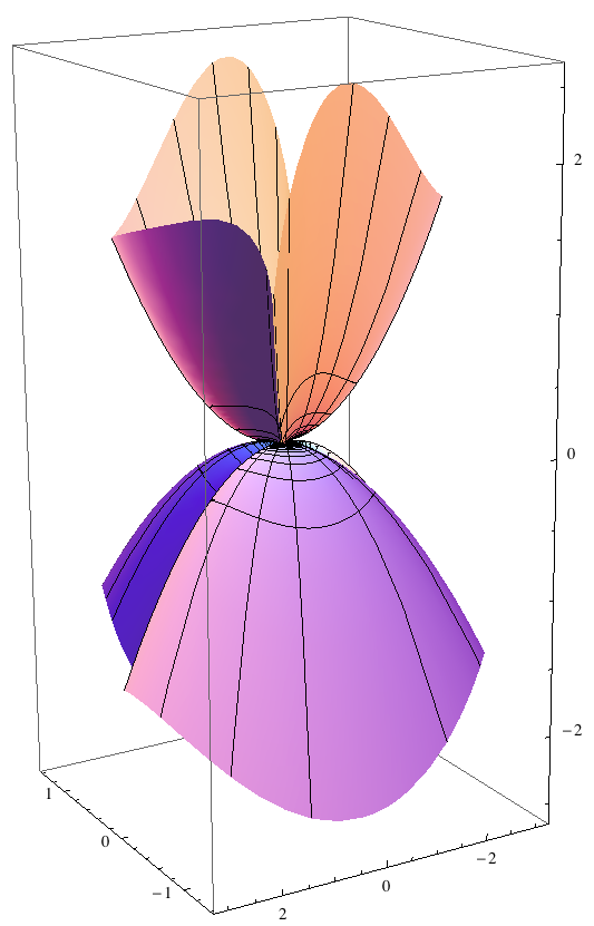
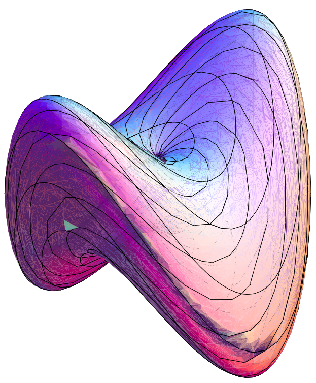
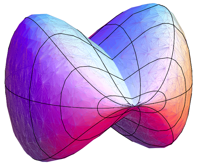
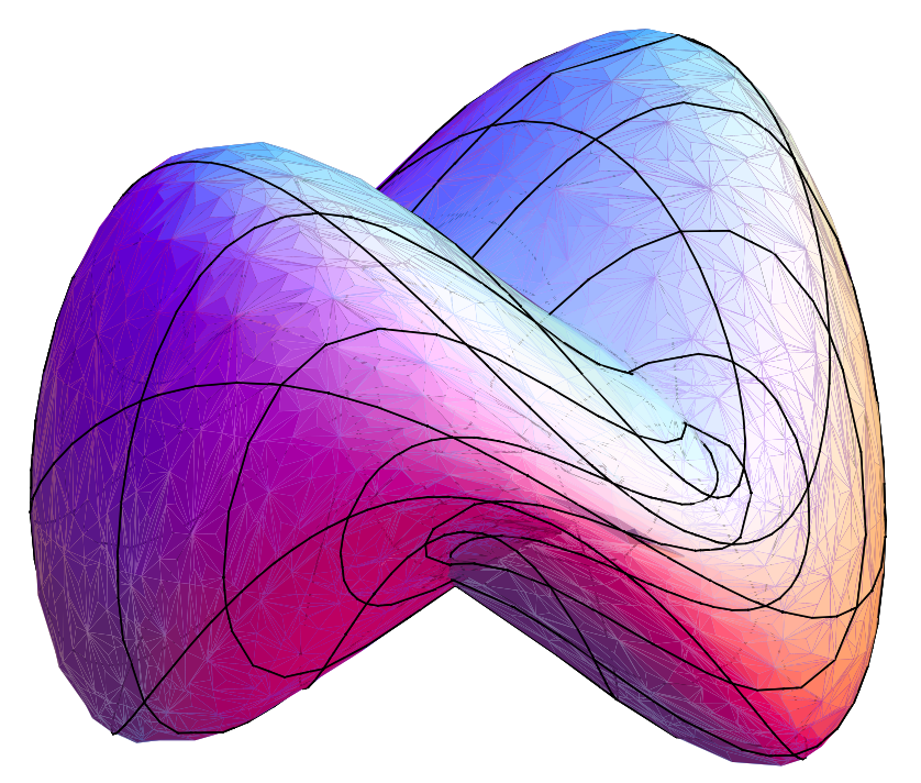
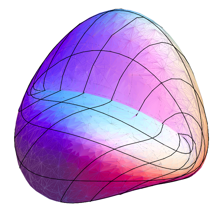
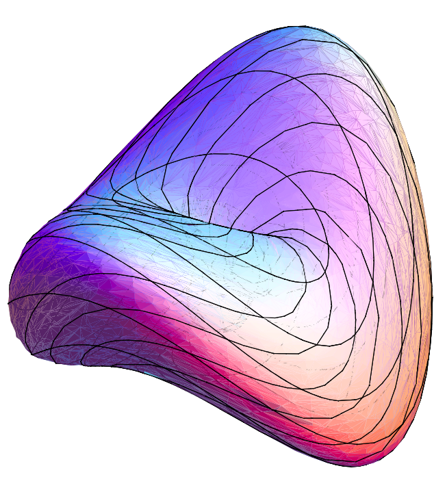
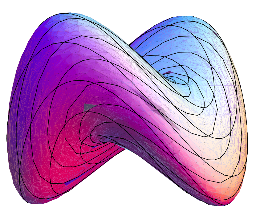
5.3 Images of the balls in the nilpotent cases

In the Riemannian case, the balls are the one of the Euclidean case. In the type-2 case, $\hat{X}_{3}$ being null and the couple $(\hat{X}_{1},\hat{X}_{2})$ being one representation of the Heisenberg metric, the balls are those of the Heisenberg case in the corresponding representation. For what concerns the type-1 case, the nilpotent approximation has a parameter $\sigma$ and the balls vary with the $\sigma$.

Refer to caption
Refer to caption
Figure 4: The spheres in the case $\sigma=0$ (Heisenberg) and $\sigma=\pi/2$ (Baouendi-Goulaouic)
Refer to caption
Refer to caption
Figure 5: Two points of view of the case $\sigma=1$
Refer to caption
Refer to caption
Figure 6: Two points of view of the case $\sigma=0,5$

6 Some Remarks on the heat diffusion

In this section we briefly discuss the heat diffusion on 3-ARSs.

For a sub-Riemannian manifold, the Laplace operator is defined as the divergence of the horizontal gradient [2, 22]. The divergence is computed with respect to a given volume, while the horizontal gradient is computed using an orthonormal frame $\{X_{1},\ldots,X_{m}\}$ via the formula grad${}_{H}(\phi)=\sum_{i}^{m}X_{i}(\phi)X_{i}$.

In particular in the case of 3-ARSs, we have the following.

Definition 8

Consider a 3-ARS on a smooth manifold $M$. Let $\{X_{1},X_{2},X_{3}\}$ be an orthonormal frame defined in an open set $U\subset M$ and let $\mu$ be a smooth volume on $M$. Then the Laplacian on $U$ is defined as

$$\Delta_{\mu}\phi=\mbox{div${}_{\mu}$(grad}_{H}(\phi))=\sum_{i=1}^{3}\left(X_{i}^{2}+\mbox{div${}_{\mu}$}(X_{i})X_{i}\right)\phi$$

Here divμ is the divergence with respect to the volume $\mu$.

Remark 7

We recall that if $X=(X^{1}(x,y,z),X^{2}(x,y,z),X^{3}(x,y,z))$ and $\mu=h(x,y,z)dx\,dy\,dz$ then

$$\mbox{div}_{\mu}X=\frac{1}{h}\left(\partial_{x}(hX^{1})+\partial_{y}(hX^{2})+\partial_{z}(hX^{3})\right).$$

It is easy to check that the definition of $\Delta_{\mu}$ does not depend on the choice of the orthonormal frame and that $\Delta_{\mu}$ is well defined on the whole manifold $M$.

By direct application of the Hormander theorem [30] (thanks to the fact that $\{X_{1},X_{2},X_{3}\}$ is bracket generating) and using a theorem of Strichartz [37], we have the following.

Theorem 6 (Hormander-Strichartz)

Consider a 3-ARS that is complete as metric space. Let $\mu$ be a smooth volume on $M$. Then $\Delta_{\mu}$ is hypoelliptic and it is essentially self-adjoint on $L^{2}(M,\mu)$. Moreover the unique solution to the Cauchy problem

$\displaystyle\left\{\begin{array}[]{l}(\partial_{t}-\Delta_{\mu})\phi=0\\ \phi(q,0)=\phi_{0}(q)\in L^{2}(M,\mu)\cap L^{1}(M,\mu),\end{array}\right.$ (42)

on $[0,\infty[\times M$ can be written as

$$\phi(q,t)=\int_{M}\phi_{0}(\bar{q})K_{t}(q,\bar{q})\,\mu(\bar{q})$$

where $K_{t}(q,\bar{q})$ is a positive function defined on $]0,\infty[\times M\times M$ which is smooth, symmetric for the exchange of $q$ and $\bar{q}$ and such that for every fixed $t,q$, we have $K_{t}(q,\cdot)\in L^{2}(M,\mu)\cap L^{1}(M,\mu)$.

Theorem 6 gives important information on the heat diffusion. Even more, one can relate the heat-kernel asymptotics with the Carnot Caratheodory distance, using the theory developed in [11, 13, 14, 32, 33]. For instance a result due to Leandre [32, 33] says that

$\displaystyle\lim_{t\to 0}\Big{(}-4t\log K_{t}(q_{1},q_{2})\Big{)}=d(q_{1},q_{2})$ (43)

In some cases an integral representation for the heat kernel can also be obtained (see Appendix B for the case of nilpotent structures for type-1 points,222 Notice that, in the nilpotent case, if one uses the Lebesgue volume, type-1 points are the only interesting ones. Indeed the heat kernel for the nilpotent approximation for Riemannian points is well known and type-2 points are a particular case of type-1 points. with respect to the Lebesgue volume in $\mathbb{R}^{3}$).

It should be noticed that the definition of the Laplacian given in Definition 8 is not completely satisfactory, due to the need of an external volume $\mu$. One would prefer to define a more intrinsic Laplacian depending only on the 3-ARS.

An intrinsic choice of volume exists. It is the Riemannian volume $\omega$ associated with the local orthonormal frame $X_{1},X_{2},X_{3}$. However this volume is well defined only on $M\setminus\mathcal{Z}$. See formula (29) for its expression using the local representation given by Theorem 2. Hence the Lapacian $\Delta_{\omega}$ (that we call the intrinsic Laplacian) contains some diverging first order terms and it is well defined only on $M\setminus\mathcal{Z}$. Using the local representation given by theorem 2 we obtain,

$$\Delta_{\omega}=\partial_{x}^{2}+(\alpha\partial_{y}+\beta\partial_{z})^{2}+\nu^{2}\partial_{z}^{2}-\frac{\partial_{x}(\alpha\nu)}{\alpha\nu}\partial_{x}+(-\alpha\frac{\partial_{y}\nu}{\nu}+\partial_{z}\beta-\beta\frac{\partial_{z}(\alpha\nu)}{\alpha\nu})(\alpha\partial_{y}+\beta\partial_{z})-\frac{\nu^{2}}{\alpha}\partial_{z}\alpha\,\partial_{z}.$$

Theorem 6 does not apply to $\Delta_{\omega}$. This operator is not well defined on the whole manifold. Theorem 6 cannot be applied even on a connected component $\Omega$ of $M\setminus\mathcal{Z}$. Indeed due to the fact that the geodesics can cross the singular set, it happens that in general the 3-ARS restricted to $\Omega$, is not complete as metric space.

These facts are well known in dimension 2 [22], together with the fact that $\mathcal{Z}$ behaves as a barrier for the heat flow.

In dimension 3 we are going to illustrate that the same phenomenon occurs for the nilpotent structure of type-1 points. The fact that $\mathcal{Z}$ behaves as a barrier for the heat flow is probably true in much more general situations, but this discussion is out of the purpose of this paper.

Theorem 7

On $\mathbb{R}^{3}$ consider the 3-ARS defined by the following 3 vector fields

X^1(x,y,z)=(100),X^2(x,y,z)=(01cos(σ)x),X^3(x,y,z)=(00sin(σ)x),formulae-sequencesubscript^𝑋1𝑥𝑦𝑧100formulae-sequencesubscript^𝑋2𝑥𝑦𝑧01𝜎𝑥subscript^𝑋3𝑥𝑦𝑧00𝜎𝑥\hat{X}_{1}(x,y,z)=\left(\begin{array}[]{c}1\\ 0\\ 0\end{array}\right),~{}~{}~{}\hat{X}_{2}(x,y,z)=\left(\begin{array}[]{c}0\\ 1\\ \cos(\sigma)x\end{array}\right),~{}~{}~{}\hat{X}_{3}(x,y,z)=\left(\begin{array}[]{c}0\\ 0\\ \sin(\sigma)x\end{array}\right),

where $\sigma\in]0,\pi/2]$ is a parameter. The corresponding Riemannian volume (defined on $\mathbb{R}^{3}\setminus\{x=0\}$) is

$$\omega=\frac{1}{\sin(\sigma)|x|}dx\,dy\,dz$$

The intrinsic Laplacian has the expression

$$\Delta_{\omega}=\partial_{x}^{2}+(\partial_{y}+\cos(\sigma)x\,\partial_{z})^{2}+\sin(\sigma)^{2}x^{2}\partial_{z}^{2}-\frac{1}{x}\partial_{x}.$$

This operator with domain ${{\mathcal{C}}^{\infty}_{c}}(\mathbb{R}^{3}\setminus\{x=0\})$ is essentially self-adjoint in $L^{2}(\mathbb{R}^{3}\setminus\{x=0\})$. Hence it separates in the direct sum of its restrictions to $\mathbb{R}^{3}\setminus\{x<0\}$ and $\mathbb{R}^{3}\setminus\{x>0\}$.

Proof. Let us make the change of variable in Hilbert space $f=\sqrt{\sin(\sigma)|x|}g$ which is unitary from $L^{2}(\mathbb{R}^{3},\omega)$ to $L^{2}(\mathbb{R}^{3},dx\,dy\,dz)$, so that $(f_{1},f_{2})_{L^{2}(\mathbb{R}^{3},\omega)}=(g_{1},g_{2})_{L^{2}(\mathbb{R}^{3},dx\,dy\,dz)}$.

We compute the operator in the new variable:

$\displaystyle\Delta_{\omega}f$ $\displaystyle=$ $\displaystyle\Big{(}\partial_{x}^{2}+(\partial_{y}+\cos(\sigma)x\,\partial_{z})^{2}+\sin(\sigma)^{2}x^{2}\partial_{z}^{2}-\frac{1}{x}\partial_{x}\Big{)}f=$
$\displaystyle=$ $\displaystyle\sqrt{\sin(\sigma)|x|}\Big{(}\partial_{x}^{2}+(\partial_{y}+\cos(\sigma)x\,\partial_{z})^{2}+\sin(\sigma)^{2}x^{2}\partial_{z}^{2}-\frac{3}{4x^{2}}\Big{)}g=:\sqrt{\sin(\sigma)|x|}Lg.$

Hence we are left to study the operator $Lg=\Big{(}\partial_{x}^{2}+(\partial_{y}+\cos(\sigma)x\,\partial_{z})^{2}+\sin(\sigma)^{2}x^{2}\partial_{z}^{2}-\frac{3}{4x^{2}}\Big{)}g$ on $L^{2}(\mathbb{R}^{3},dx\,dy\,dz)$. By making the Fourier transform in $y$ and $z$, we have $\partial_{y}\to i\mu$, $\partial_{z}\to i\nu$, we are left to study the operator

$\displaystyle\hat{L}^{\mu,\nu}=\partial_{x}^{2}-(\mu+\cos(\sigma)\nu x)^{2}-\sin(\sigma)^{2}\nu^{2}x^{2}-\frac{3}{4x^{2}}=\partial_{x}^{2}-V^{\mu,\nu}(x).$

with $V^{\mu,\nu}(x)\geq\frac{3}{4x^{2}}$. But in dimension $1$ the operator $-\partial_{x}^{2}+V$ with domain $C^{\infty}_{0}(]0,+\infty[)$ is essentially self-adjoint on $L^{2}(]0,+\infty[)$ if $V\geq\frac{3}{4x^{2}}$ (see [36], Theorem X.10 for the proof of the limit point case at 00 and Theorem X.8 at $+\infty$). Hence, each operator $L^{\mu,\nu}$ is essentially self-adjoint in $]0,+\infty[$ . As a consequence $L^{\mu,\nu}$ is essentially self-adjoint in $]-\infty,+\infty[$ and it separates in the direct sum of its restrictions to $]-\infty,0[$ and $]0,+\infty[$. By making the inverse Fourier transform, the thesis follows. $\Box$

As a direct consequence we have the following

Corollary 1

With the notations of Theorem 7, consider the unique solution $\phi$ of the heat equation (according to the self-adjoint extension defined in the previous theorem),

$\displaystyle\partial_{t}\phi-\Delta_{\omega}\phi$ $\displaystyle=$ $\displaystyle 0$ (44)
$\displaystyle\phi(0)$ $\displaystyle=$ $\displaystyle\phi_{0}\in L^{2}(\mathbb{R}^{3},\omega)\cap L^{1}(\mathbb{R}^{3},\omega)$ (45)

with $\phi_{0}$ supported in $\mathbb{R}^{3}\setminus\{x<0\}$. Then, $\phi(t)$ is supported in $\mathbb{R}^{3}\setminus\{x<0\}$ for any $t\geq 0$. The same holds for the solution of the Schroedinger equation or for the solution of the wave equation.

Hence formula (43) does not apply for the diffusion generated by the intrinsic Laplacian. Indeed for type-1 points in the nilpotent case, the heat does not flow through $\{x=0\}$, while the Carnot Caratheodory distance is finite for every pair of points.

Appendix A Genericity of (G1),(G2),(G3)

In this part, we provide a proof of Proposition 1. Before that, we first give some basic results on transversality theory.

A.1 Thom Transversality Theorem

Let $M$ and $N$ be smooth manifolds and $k\geq 0$ be an integer. Let $x\in M$, $y\in N$ and $C^{\infty}(M,N,x,y)$ be the set of smooth maps from $M$ to $N$ which send $x$ to $y$. Let $\varphi$ and $\psi$ be local charts of $M$ and $N$ around $x$ and $y$ respectively.

We use $\mathcal{R}_{k}$ to define the following equivalence relation on $C^{\infty}(M,N,x,y)$: Two functions $f$ and $g$ are equivalent if the functions $\psi\circ f\circ\varphi^{-1}$ and $\psi\circ g\circ\varphi^{-1}$ have the same partial derivatives at any order less or equal to $k$ at $\varphi(x)$.

Remark 8

Notice that ${\mathcal{R}}_{k}$ is independent of the choice of the charts $\varphi$ and $\psi$.

In order to state the Thom Transversality Theorem, we need to list some definitions.

Definition 9

Let $M$ and $N$ smooth manifolds. A jet at order $k$ from $M$ to $N$ is a triplet $(x,y,u)$ where $x\in M$, $y\in N$ and $u$ is an equivalence class (for ${\mathcal{R}}_{k}$) of the functions $C^{\infty}(M,N,x,y)$.

A $k$-th order jet space from $M$ to $N$ denoted by $J^{k}(M,N)$ is the set of jets at order $k$ from $M$ to $N$.

Proposition 2 ([29])

Let $M$ and $N$ smooth manifolds and $k\geq 0$ an integer. Then $J^{k}(M,N)$ has a structure of smooth manifold.

Definition 10

Let $M$ and $N$ smooth manifolds.

  • $(i)$

    We say that a subset of $C^{\infty}(M,N)$ is residual (and hence dense) if it is an intersection of open dense subsets of $C^{\infty}(M,N)$ endowed with the $C^{\infty}$-Whitney topology.

  • $(ii)$

    We say that $f\in C^{\infty}(M,N)$ is transverse to a smooth submanifold $S$ of $N$ at $x\in M$ if either $f(x)\notin S$ or $y:=f(x)\in S$ and $Df(x)(T_{x}M)+T_{y}S=T_{y}N$. If $f$ is transverse to $S$ at every point of $M$ then we say that $f$ is transverse to $S$ and we denote it by $f\pitchfork S$. Moreover $f^{-1}(S)$ is a submanifold of $M$ with the same codimension as $S$.

  • $(iii)$

    If $f\in C^{\infty}(M,N)$ then its $k$-jet extension $J^{k}f$ is the smooth map from $M$ to $J^{k}(M,N)$ which assigns to every $x\in M$ the jet of $f$ of order $k$ at $x$.

Theorem 8 (Thom Transversality Theorem, [29], Page 82)

Let $M,N$ smooth manifolds and $k\geq 1$ an integer. If $S_{1},\cdots,S_{r}$ are smooth submanifolds of $J^{k}(M,N)$ then the set

$\displaystyle\{f\in C^{\infty}(M,N):J^{k}f\pitchfork S_{i}~{}\text{for}~{}i=1,2,\cdots,r\},$ (46)

is residual in the $C^{\infty}$-Whitney topology.

If codim$\ S_{i}>\dim M$ then $J^{k}f\pitchfork S_{i}$ means that $J^{k}f(M)\cap S_{i}=\emptyset$. Hence, we have:

Corollary 2

Assume that $codim\ S_{i}>\dim M$ for $i=1,\cdots,r$ and $k\geq 1$. Then the set

$$\{f\in C^{\infty}(M,N):J^{k}f\cap S_{i}=\emptyset~{}\text{for}~{}i=1,2,\cdots,r\},$$ (47)

is residual in the $C^{\infty}$-Whitney topology.

By using Item $(ii)$ of Definition 10 and Theorem 8 , we have the following:

Corollary 3

For every $f$ in the residual set defined in Theorem 8, the inverse images $\tilde{S_{i}}:=(J^{k}f)^{-1}(S_{i})$ is a smooth submanifold of $M$ and $codim\ S_{i}=codim\ \tilde{S}_{i}$ for $i=1,\cdots,r$.

A.2 Proof of Proposition 1

Here $M$ is a fixed $3$-dimensional smooth manifold. We use $N$ and $C^{\infty}(M,N)$ to denote the smooth manifold $\underset{q\in M}{\bigcup}N_{q}$ of dimension $12$, where $N_{q}:=(T_{q}M)^{3}$, and the set of smooth maps from $M$ to $N$ which assign to every $q\in M$ an element of $N_{q}$, respectively. Let recall the conditions (G1), (G2) and (G3):

(G1) dim($\blacktriangle(q))\geq 2$ and $\blacktriangle(q)+[\blacktriangle,\blacktriangle](q)=T_{q}M$ for every $q\in M$;

(G2) $\mathcal{Z}$ is an embedded two-dimensional submanifold of $M$;

(G3) the points where $\blacktriangle(q)=T_{q}\mathcal{Z}$ are isolated.

Proof of Property (G1): Let us now prove the first part. For this purpose, consider the smooth submanifold of $J^{1}(M,N)$ of codimension $9$ defined as follows:

$$S_{1}:=\{J^{1}(X_{1},X_{2},X_{3})(q)\in J^{1}(M,N):(X_{1}(q),X_{2}(q),X_{3}(q))=0\in N_{q}\}.$$

Then by using Corollary 2, we obtain that

$$\mathcal{O}_{1}:=\{(X_{1},X_{2},X_{3})\in C^{\infty}(M,N):J^{1}(X_{1},X_{2},X_{3})(M)\cap S_{1}=\emptyset\},$$

is a residual subset of $C^{\infty}(M,N)$ endowed with the $C^{\infty}$-Whitney topology. We next define the set

$$S_{2}:=\left\{J^{1}(X_{1},X_{2},X_{3})(q)\in J^{1}(M,N):\begin{array}[]{l}(X_{1}(q),X_{2}(q),X_{3}(q))\neq 0\in N_{q},\\ ~{}~{}~{}~{}X_{1}(q)\wedge X_{2}(q)=0,\\ ~{}~{}~{}~{}X_{1}(q)\wedge X_{3}(q)=0,\\ ~{}~{}~{}~{}X_{2}(q)\wedge X_{3}(q)=0.\end{array}\right\},$$

and we easily prove that it is a smooth submanifold of $J^{1}(M,N)$ of codimension strictly greater than $3$. Therefore we have that the set

$$\mathcal{O}_{2}:=\{(X_{1},X_{2},X_{3})\in C^{\infty}(M,N):J^{1}(X_{1},X_{2},X_{3})(M)\cap S_{2}=\emptyset\},$$

is a residual subset of $C^{\infty}(M,N)$ in the $C^{\infty}$-Whitney topology. Thus, for every $(X_{1},X_{2},X_{3})\in\mathcal{O}:=\mathcal{O}_{1}\cap\mathcal{O}_{2}$, we have that $J^{1}(X_{1},X_{2},X_{3})(q)\notin S_{1}$ and $J^{1}(X_{1},X_{2},X_{3})(q)\notin S_{2}$. Hence we conclude the first part of $(\textbf{G1})$.

We next prove the second step. As above, we define the following subset of $J^{1}(M,N)$:

$$S:=\left\{J^{1}(X_{1},X_{2},X_{3})(q)\in J^{1}(M,N):\begin{array}[]{l}~{}~{}(X_{1}(q)\wedge X_{2}(q),X_{1}(q)\wedge X_{3}(q),X_{2}(q)\wedge X_{3}(q))\neq 0,\\ \det(X_{1}(q),X_{2}(q),X_{3}(q))=0,~{}\text{and for}~{}1\leq i<j\leq 3,\\ ~{}~{}~{}~{}~{}~{}~{}~{}\det(X_{i}(q),X_{j}(q),[X_{1},X_{2}](q))=0,\\ ~{}~{}~{}~{}~{}~{}~{}~{}\det(X_{i}(q),X_{j}(q),[X_{1},X_{3}](q))=0,\\ ~{}~{}~{}~{}~{}~{}~{}~{}\det(X_{i}(q),X_{j}(q),[X_{2},X_{3}](q))=0.\end{array}\right\}.$$

By the same strategy as in the first part, we can easily see that $S$ is a smooth submanifold of $J^{1}(M,N)$ with codimension $4$. Thanks to Corollary 2

$$\mathcal{P}:=\{(X_{1},X_{2},X_{3})\in C^{\infty}(M,N):J^{1}(X_{1},X_{2},X_{3})(M)\cap S=\emptyset\},$$

is a residual subset of $C^{\infty}(M,N)$ endowed with the $C^{\infty}$-Whitney topology. Let us denote by $\mathcal{A}$ the residual set $\mathcal{P}\cap\mathcal{O}$, where $\mathcal{O}$ is defined in the previous part. Hence we conclude that Span$\{X_{1}(q),X_{2}(q),X_{3}(q),[X_{1},X_{2}](q),[X_{1},X_{3}](q),[X_{2},X_{3}](q)\}=T_{q}M$, for every $(X_{1},X_{2},X_{3})\in\mathcal{A}$ and for every $q\in M$ such that $\det(X_{1}(q),X_{2}(q),X_{3}(q))=0$. This proves the second part of $(\textbf{G1})$.

Proof of Property (G2): For every $(X_{1},X_{2},X_{3})\in C^{\infty}(M,N)$, we use $\psi_{(X_{1},X_{2},X_{3})}$ and $\bar{S}$ respectively to denote the smooth map

$$q\in M\rightarrow\det(X_{1}(q),X_{2}(q),X_{3}(q))\in\mathbb{R}.$$

and the set

$$\left\{J^{1}(X_{1},X_{2},X_{3})(q)\in J^{1}(M,N):\begin{array}[]{l}(X_{1}(q)\wedge X_{2}(q),X_{1}(q)\wedge X_{3}(q),X_{2}(q)\wedge X_{3}(q))\neq 0,\\ ~{}~{}~{}~{}~{}~{}~{}~{}~{}~{}~{}~{}~{}~{}~{}~{}~{}~{}~{}~{}~{}D\psi_{(X_{1},X_{2},X_{3})}(q)=0,\\ ~{}~{}~{}~{}~{}~{}~{}~{}~{}~{}~{}~{}~{}~{}~{}~{}~{}~{}~{}~{}~{}~{}~{}~{}\psi_{(X_{1},X_{2},X_{3})}(q)=0.\end{array}\right\}.$$

Then $\bar{S}$ is a smooth submanifold of $J^{1}(M,N)$ of codimension $4$ which implies that the set

$$\bar{\mathcal{O}}:=\{(X_{1},X_{2},X_{3})\in C^{\infty}(M,N):J^{1}(X_{1},X_{2},X_{3})(M)\cap\bar{S}=\emptyset\},$$

is a residual subset of $C^{\infty}(M,N)$ in the $C^{\infty}$-Whitney topology. Let $\bar{\mathcal{A}}:=\bar{\mathcal{O}}\cap\mathcal{O}$ and $(X_{1},X_{2},X_{3})\in~{}\bar{\mathcal{A}}$. Thus, for every $q\in M$ such that $\psi_{(X_{1},X_{2},X_{3})}(q)=0$ we obtain that $D\psi_{(X_{1},X_{2},X_{3})}(q)\neq 0$. This implies that $\psi_{(X_{1},X_{2},X_{3})}$ is transverse to $\{0\}\subset\mathbb{R}$. Hence the inverse image

$$\{q\in M:\det(X_{1}(q),X_{2}(q),X_{3}(q))=0\},$$

is an embedded submanifold of $M$ of codimension $1$. This proves Property $(\textbf{G2})$.

Proof of Property (G3): We use the same techniques as previously by considering the following smooth submanifold of $J^{1}(M,N)$ of codimension $3$:

$$\tilde{S}:=\left\{J^{1}(X_{1},X_{2},X_{3})(q)\in J^{1}(M,N):\begin{array}[]{l}~{}~{}(X_{1}(q)\wedge X_{2}(q),X_{1}(q)\wedge X_{3}(q),X_{2}(q)\wedge X_{3}(q))\neq 0,\\ \det(X_{1}(q),X_{2}(q),X_{3}(q))=0,~{}\text{and for}~{}1\leq i\leq 3,\\ ~{}~{}~{}~{}~{}~{}~{}~{}\det(DX_{1}(q)X_{i}(q),X_{2}(q),X_{3}(q))\\ ~{}~{}~{}~{}~{}~{}~{}~{}+\det(X_{1}(q),DX_{2}(q)X_{i}(q),X_{3}(q))\\ ~{}~{}~{}~{}~{}~{}~{}~{}+\det(X_{1}(q),X_{2}(q),DX_{3}(q)X_{i}(q))=0.\end{array}\right\}.$$

Then by Theorem 8,

$$\tilde{\mathcal{O}}:=\{(X_{1},X_{2},X_{3})\in C^{\infty}(M,N):J^{1}(X_{1},X_{2},X_{3})\pitchfork\tilde{S}\}\cap\mathcal{\bar{A}},$$

is a residual subset of $C^{\infty}(M,N)$ in the $C^{\infty}$-Whitney topology. Now we consider the smooth maps $(X_{1},X_{2},X_{3})\in\tilde{\mathcal{O}}$. Then, by Corollary 3, $J^{1}(X_{1},X_{2},X_{3})^{-1}(\tilde{S})$ is a smooth submanifold of $M$ of codimension  $3$, i.e., it is formed by isolated points. On the other hand notice that

$$J^{1}(X_{1},X_{2},X_{3})^{-1}(\tilde{S})=\left\{q\in M:\begin{array}[]{l}\det(X_{1}(q),X_{2}(q),X_{3}(q))=0,~{}\text{and for}~{}1\leq i\leq 3,\\ ~{}~{}~{}~{}~{}~{}~{}~{}\det(DX_{1}(q)X_{i}(q),X_{2}(q),X_{3}(q))\\ ~{}~{}~{}~{}~{}~{}~{}~{}+\det(X_{1}(q),DX_{2}(q)X_{i}(q),X_{3}(q))\\ ~{}~{}~{}~{}~{}~{}~{}~{}+\det(X_{1}(q),X_{2}(q),DX_{3}(q)X_{i}(q))=0.\end{array}\right\},$$

is the set of points $q\in\mathcal{Z}$ such that $span\{X_{1}(q),X_{2}(q),X_{3}(q)\}=T_{q}\mathcal{Z}$. Here $\mathcal{Z}$ is the two dimensional embedded submanifold $\{q\in M:\det(X_{1}(q),X_{2}(q),X_{3}(q))=0\}$. Hence $(\textbf{G3})$ is proved.

Appendix B Explicit expressions of heat kernels

In this section, we consider the nilpotent structures of type-$1$ points, and the Laplacian

$$\Delta_{{\mathrm{L}}}:=\partial_{x}^{2}+(\partial_{y}+x\cos(\sigma)\partial_{z})^{2}+(x\sin(\sigma)\partial_{z})^{2}.$$ (48)

with respect to the Lebesgue volume $dv=dx\,dy\,dz$ in $\mathbb{R}^{3}$. In order to give an explicit formula of the associated heat kernel, we first introduce the following intermediate functions:

$$F(\nu,t):=-t\sin^{2}\sigma-\frac{\tanh(\nu t)\cos^{2}\sigma}{\nu},~{}~{}~{}G(\nu,t):=-\cos\sigma\tanh(\nu t),$$

defined on $(\mathbb{R}\setminus\{0\})\times]0,+\infty[$. Observe that $F(\nu,t)<0$ for every $\nu\neq 0$ and $t>0$. This comes from the fact that $\frac{\tanh(x)}{x}>0$ for every $x\neq 0$.

Let us also define the next function defined on $]0,+\infty[\times\mathbb{R}^{3}\times\mathbb{R}^{3}\times(\mathbb{R}\setminus\{0\})$:

$\displaystyle I(t;x,y,z;\bar{x},\bar{y},\bar{z};\nu):$ $\displaystyle=$ $\displaystyle\frac{1}{(2\pi)^{2}}\cos\left(\nu(z-\bar{z})-(x+\bar{x})(y-\bar{y})\frac{G(\nu,t)}{2F(\nu,t)}\right)$
$\displaystyle\times\exp\left(x\bar{x}\left(\frac{\nu}{\sinh(2\nu t)}-\frac{G^{2}(\nu,t)}{2F(\nu,t)}\right)-(x^{2}+\bar{x}^{2})\left(\frac{\nu}{2\tanh(2\nu t)}+\frac{G^{2}(\nu,t)}{4F(\nu,t)}\right)\right)$
$\displaystyle\times\exp\left(\frac{(y-\bar{y})^{2}}{4F(\nu,t)}\right)\times\left(\frac{-\nu}{2F(\nu,t)\sinh(2\nu t)}\right)^{\frac{1}{2}}.$

Thus, thanks to Theorem 6 we have the following:

Theorem 9

The unique solution of the Cauchy problem

$\displaystyle\left\{\begin{array}[]{l}(\partial_{t}-\Delta_{\mathrm{L}})\phi=0\\ \phi(x,y,z,0)=\phi_{0}(x,y,z)\in L^{2}(\mathbb{R}^{3},dv)\cap L^{1}(\mathbb{R}^{3},dv),\end{array}\right.$ (51)

defined on $\mathbb{R}^{3}\times[0,\infty[$ is of the form

$$\phi(x,y,z,t)=\int_{\mathbb{R}^{3}}\phi_{0}(\bar{x},\bar{y},\bar{z})K_{t}(x,y,z;\bar{x},\bar{y},\bar{z})\,d{\bar{x}}\ d{\bar{y}}\ d{\bar{z}},$$

where

$\displaystyle K_{t}(x,y,z;\bar{x},\bar{y},\bar{z})=\int_{\mathbb{R}}{I(t,x,y,z;\bar{x},\bar{y},\bar{z},\nu)}\ d\nu.$ (52)

Proof. Let $\phi$ and $\hat{\phi}$ the solution of Problem (51) and its Fourier transform. Applying the inverse Fourier transform only on $y$ and $z$, we get that

$$\phi(x,y,z,t)=\frac{1}{(2\pi)^{2}}\int_{\mathbb{R}^{2}}\exp(i(\mu y+\nu z))\hat{\phi}(x,\mu,\nu,t)\ d\mu\ d\nu.$$

Thus, we easily prove that Problem (51) is equivalent to the following:

$\displaystyle\left\{\begin{array}[]{l}\partial_{t}{\hat{\phi}(x,\mu,\nu,t)}=(\partial_{x}^{2}-(\nu x+\mu\cos\sigma)^{2}-\mu^{2}\sin^{2}\sigma)\hat{\phi}(x,\mu,\nu,t),\\ \hat{\phi}(x,\mu,\nu,0)={\hat{\phi}}_{0}(x,\mu,\nu)\in L^{2}(\mathbb{R}^{3},\mathbb{R})\cap L^{1}(\mathbb{R}^{3},\mathbb{R}).\end{array}\right.$ (55)

Hence, by making the change of variable $x\rightarrow\gamma=x+\frac{\mu}{\nu}\cos\sigma$ ($\nu\neq 0$), Problem (55) becomes:

$\displaystyle\left\{\begin{array}[]{l}\partial_{t}\ {\bar{\phi}^{\mu,\nu}(\gamma,t)}=\left({\partial_{\gamma}}^{2}-\nu^{2}\gamma^{2}-\mu^{2}\sin^{2}\sigma\right)\bar{\phi}^{\mu,\nu}(\gamma,t),\\ \bar{\phi}^{\mu,\nu}(\gamma,0)=\bar{\phi}_{0}^{\mu,\nu}(\gamma),\end{array}\right.$ (58)

where

$$\bar{\phi}^{\mu,\nu}(\gamma,t):=\hat{\phi}(\gamma-\frac{\mu}{\nu}\cos\sigma,\mu,\nu,t)~{}~{}\text{and}~{}~{}\bar{\phi}_{0}^{\mu,\nu}(\gamma):={\hat{\phi}}_{0}(\gamma-\frac{\mu}{\nu}\cos\sigma,\mu,\nu).$$

In the sequel, we use $\psi(\gamma,t)$ to denote the solution of Problem (58). First remark that the eigenvalues and the associated eigenfunctions of the operator $\partial_{\gamma}^{2}-\nu^{2}\gamma^{2}-\mu^{2}\sin^{2}\sigma$ ($\nu\neq 0$ ) on $\mathbb{R}$ are respectively given by

$$E_{n}=-2\nu(n+\frac{1}{2})-\mu^{2}\sin^{2}\sigma,$$

and

$$\phi_{n}^{\nu}(\gamma):=\frac{1}{\sqrt{2^{n}n\mathpunct{}!}}\left(\frac{\nu}{\pi}\right)^{\frac{1}{4}}\exp(-\frac{\nu\gamma^{2}}{2})\ H_{n}(\gamma\sqrt{\nu})~{}~{}\text{where}~{}~{}H_{n}(\gamma):=(-1)^{n}e^{\gamma^{2}}\frac{d^{n}}{d\gamma^{n}}\exp(-\gamma^{2}),~{}~{}n=0,1,\cdots.$$

Since the sequence $\{\phi_{n}^{\nu}\}_{n}$ is an orthonormal basis of $L^{2}(\mathbb{R})$ then there exists a sequence of functions $\{C_{n}(\cdot)\}_{n}$ such that $\psi(\gamma,t)=\sum_{n\geq 0}{C_{n}(t)\phi_{n}^{\nu}(\gamma)}$. According to Problem (58), we easily obtain that $\dot{C_{n}}(t)=E_{n}C_{n}(t)$ which implies that $C_{n}(t)=\exp(tE_{n})C_{n}(0)$ for $n\in\mathbb{N}$ and $t\geq 0$. The fact that

$$C_{n}(0)=\int_{\mathbb{R}}\psi_{0}(\bar{\gamma})\phi_{n}^{\nu}(\bar{\gamma})d{\bar{\gamma}},$$

implies after simple computations that

$$\psi(\gamma,t)=\int_{\mathbb{R}}\psi_{0}(\bar{\gamma}){Q_{t}}^{\mu,\nu}(\gamma,\bar{\gamma})\ d{\bar{\gamma}}~{}~{}\text{with}~{}~{}{Q_{t}}^{\mu,\nu}(\gamma,\bar{\gamma})=\left(\sum_{n\geq 0}{\exp(tE_{n})\ \phi_{n}^{\nu}(\gamma)\ \phi_{n}^{\nu}(\bar{\gamma})}\right).$$

Thus, we obtain that

$${Q_{t}}^{\mu,\nu}(\gamma,\bar{\gamma})=\left(\frac{\nu}{\pi}\right)^{\frac{1}{2}}\exp\left(-\frac{\nu}{2}(\gamma^{2}+\bar{\gamma}^{2}+2t)-t\mu^{2}\sin^{2}\sigma\right)\ \sum_{n\geq 0}{\exp(-2t\nu n)}\ \frac{1}{2^{n}n\mathpunct{}!}\ H_{n}(\gamma\sqrt{\nu})\ H_{n}(\bar{\gamma}\sqrt{\nu}).$$

Let us denote $w=\exp(-2t\nu)$. By the Mehler’s formula we get that

$$\sum_{n\geq 0}{\exp(-2t\nu n)}\ \frac{1}{2^{n}n\mathpunct{}!}\ H_{n}(\gamma\sqrt{\nu})\ H_{n}(\bar{\gamma}\sqrt{\nu})=(1-w^{2})^{-\frac{1}{2}}\ \exp\left(\frac{2\nu\gamma\bar{\gamma}w-\nu(\gamma^{2}+\bar{\gamma}^{2})w^{2}}{1-w^{2}}\right),$$

which implies that

$${Q_{t}}^{\mu,\nu}(\gamma,\bar{\gamma})=\left(\frac{\nu}{\pi}\right)^{\frac{1}{2}}\exp\left(-\frac{\nu}{2}(\gamma^{2}+\bar{\gamma}^{2}+2t)-t\mu^{2}\sin^{2}\sigma\right)\ (1-w^{2})^{-\frac{1}{2}}\ \exp\left(\frac{2\nu\gamma\bar{\gamma}w-\nu(\gamma^{2}+\bar{\gamma}^{2})w^{2}}{1-w^{2}}\right).$$

After some algebraic computations, we deduce that

$${Q_{t}}^{\mu,\nu}(\gamma,\bar{\gamma})=\exp(-t\mu^{2}\sin^{2}\sigma)\ \left(\frac{\nu w}{\pi(1-w^{2})}\right)^{\frac{1}{2}}\ \exp\left(\frac{\nu\gamma\bar{\gamma}(w-1)}{w+1}-\frac{\nu(\gamma-\bar{\gamma})^{2}(w^{2}+1)}{2(1-w^{2})}\right).$$

Let us remark that

$$\frac{w}{1-w^{2}}=\frac{1}{2\sinh(2\nu t)},~{}~{}\frac{w-1}{1+w}=\frac{1}{\sinh(2\nu t)}-\frac{1}{\tanh(2\nu t)}=-\tanh(\nu t)~{}~{}\text{and}~{}~{}\frac{w^{2}+1}{1-w^{2}}=\frac{1}{\tanh(2\nu t)}.$$

Hence, we conclude that

$${Q_{t}}^{\mu,\nu}(\gamma,\bar{\gamma})=\left(\frac{\nu}{2\pi\sinh(2\nu t)}\right)^{\frac{1}{2}}\ \exp\left(-\left(t\mu^{2}\sin^{2}\sigma+\frac{\nu(\gamma-\bar{\gamma})^{2}}{2\tanh(2\nu t)}+\nu\tanh(\nu t)\gamma\bar{\gamma}\right)\right).$$

Since $\psi_{0}(\bar{\gamma})=\hat{\phi}_{0}(\bar{\gamma}-\frac{\mu}{\nu}\cos\sigma,\mu,\nu)$, then we have that

$$\psi_{0}(\bar{\gamma})=\int_{\mathbb{R}^{2}}{\exp(-i\mu\bar{y})\ \exp(-i\nu\bar{z})\ \phi_{0}(\bar{\gamma}-\frac{\mu}{\nu}\cos\sigma,\bar{y},\bar{z})}\ d\bar{y}\ d\bar{z},$$

which implies that

$$\bar{\phi}^{\mu,\nu}(\gamma,t)=\int_{\mathbb{R}}\left(\int_{\mathbb{R}^{2}}{\exp(-i\mu\bar{y})\ \exp(-i\nu\bar{z})\ \phi_{0}(\bar{\gamma}-\frac{\mu}{\nu}\cos\sigma,\bar{y},\bar{z})}\ d\bar{y}\ d\bar{z}\right){{Q_{t}}^{\mu,\nu}(\gamma,\bar{\gamma})}\ d\bar{\gamma}.$$ (59)

By the fact that $\bar{\phi}^{\mu,\nu}(\gamma,t)=\hat{\phi}(\gamma-\frac{\mu}{\nu}\cos\sigma,\mu,\nu,t)$ and by making the inverse Fourier transform we deduce that

$$\phi(x,y,z,t)=\frac{1}{(2\pi)^{2}}\int_{\mathbb{R}^{2}}{\exp(i\mu y)\ \exp(i\nu z)\ \bar{\phi}^{\mu,\nu}\left(x+\frac{\mu\cos\sigma}{\nu},t\right)}\ d\mu\ d\nu.$$ (60)

Hence by using the change of variable $\bar{\gamma}\rightarrow\bar{x}=\bar{\gamma}-\frac{\mu\cos\sigma}{\nu}$, and replacing Eq. (59) with $\gamma=x+\frac{\mu\cos\sigma}{\nu}$ in Eq. (60), we easily conclude that

$$\phi(x,y,z,t)=\int_{\mathbb{R}^{3}}K_{t}(x,y,z;\bar{x},\bar{y},\bar{z})\ \phi_{0}(\bar{x},\bar{y},\bar{z})\,d{\bar{x}}\ d{\bar{y}}\ d{\bar{z}},$$

where

$$K_{t}(x,y,z;\bar{x},\bar{y},\bar{z})=\frac{1}{(2\pi)^{2}}\int_{\mathbb{R}^{2}}{Q_{t}}^{\mu,\nu}(x+\frac{\mu}{\nu}\cos\sigma,\bar{x}+\frac{\mu}{\nu}\cos\sigma)\ \exp(i\mu(y-\bar{y}))\ \exp(i\nu(z-\bar{z}))\,d{\mu}\ d{\nu}.$$

Since

$\displaystyle{Q_{t}}^{\mu,\nu}(x+\frac{\mu}{\nu}\cos\sigma,\bar{x}+\frac{\mu}{\nu}\cos\sigma)$ $\displaystyle=$ $\displaystyle\exp(-t\mu^{2}\sin^{2}\sigma)\ \left(\frac{\nu}{2\pi\sinh(2\nu t)}\right)^{\frac{1}{2}}$
$\displaystyle\times\exp\left(-\left(\frac{\nu(x-\bar{x})^{2}}{2\tanh(2\nu t)}+\nu\tanh(\nu t)(x+\frac{\mu}{\nu}\cos\sigma)(\bar{x}+\frac{\mu}{\nu}\cos\sigma)\right)\right),$

then by defining

$$A(\nu,t):=\int_{\mathbb{R}}\exp(i\mu(y-\bar{y}))\exp\left(-t\mu^{2}\sin^{2}\sigma-\nu\tanh(\nu t)\left(\frac{\mu(x+\bar{x})\cos\sigma}{\nu}+\frac{\mu^{2}\cos^{2}\sigma}{\nu^{2}}\right)\right)\ d\mu,$$

we deduce that

$\displaystyle K_{t}(x,y,z;\bar{x},\bar{y},\bar{z})=\frac{1}{(2\pi)^{2}}\int_{\mathbb{R}}\exp(i\nu(z-\bar{z}))\left(\frac{\nu}{2\pi\sinh(2\nu t)}\right)^{\frac{1}{2}}\exp\left(-\frac{\nu(x-\bar{x})^{2}}{2\tanh(2\nu t)}-\nu\tanh(\nu t)x\bar{x}\right)A(\nu,t)\ d\nu.$ (61)

Let us now give a better formula of $A(\nu,t)$. By straightforward computations, we observe that

$$A(\nu,t)=\int_{\mathbb{R}}\exp(i\mu(y-\bar{y}))\exp\left(F(\nu,t)\mu^{2}+(x+\bar{x})G(\nu,t)\mu\right)\ d\mu.$$

Therefore by making the change of variable $\mu\rightarrow\xi=\mu+\frac{(x+\bar{x})\ G(\nu,t)}{2F(\nu,t)}$, we easily have that

$$A(\nu,t)=\exp\left(-\frac{(x+\bar{x})^{2}\ G^{2}(\nu,t)}{4\ F(\nu,t)}\right)\int_{\mathbb{R}}\exp\left(i\ (y-\bar{y})\left(\xi-\frac{(x+\bar{x})\ G(\nu,t)}{2\ F(\nu,t)}\right)\right)\ \exp\left(F(\nu,t)\xi^{2}\right)\ d\xi.$$

Since

$$\int_{\mathbb{R}}\exp(i\xi(y-\bar{y}))\exp\left(F(\nu,t)\xi^{2}\right)\ d\xi=\left(\frac{-\pi}{F(\nu,t)}\right)^{\frac{1}{2}}\ \exp\left(\frac{(y-\bar{y})^{2}}{4F(\nu,t)}\right),$$

we conclude that

$\displaystyle A(\nu,t)=\left(\frac{-\pi}{F(\nu,t)}\right)^{\frac{1}{2}}\ \exp\left(\frac{(y-\bar{y})^{2}}{4F(\nu,t)}-\frac{(x+\bar{x})^{2}\ G^{2}(\nu,t)}{4\ F(\nu,t)}-i\ \frac{(x+\bar{x})\ (y-\bar{y})\ G(\nu,t)}{2\ F(\nu,t)}\right).$ (62)

Hence, we obtain Eq.(52)52(\ref{NChaleur}) of Theorem 9 by replacing Eq.(62) in Eq.(61). $\Box$

Observe that the Baouendi-Goulaouic operator which is defined in (LABEL:Baouendi_Goulaouic) corresponds to $\Delta_{\mathrm{L}}$ in the case where $\sigma=\frac{\pi}{2}$. Hence, according to the previous theorem we have the following

Corollary 4

The heat kernel associated with the Baouendi-Goulaouic operator is given by

$$K_{t}(x,y,z;\bar{x},\bar{y},\bar{z}):=\displaystyle{\int_{\mathbb{R}}}{I_{B}(t;x,y,z;\bar{x},\bar{y},\bar{z};\nu)}\ d\nu,$$

where

$\displaystyle I_{B}(t;x,y,z;\bar{x},\bar{y},\bar{z};\nu):$ $\displaystyle=$ $\displaystyle\frac{1}{(2\pi)^{2}}\ cos(\nu(z-\bar{z}))\times\left(\frac{\nu}{2t\sinh(2\nu t)}\right)^{\frac{1}{2}}$
$\displaystyle\times\exp\left(\frac{\nu\ x\bar{x}}{\sinh(2\nu t)}-\frac{\nu\ (x^{2}+\bar{x}^{2})}{2\tanh(2\nu t)}-\frac{(y-\bar{y})^{2}}{4t}\right).$

Let us now consider the case where $\sigma=0$. Then we obtain the well-known Heisenberg-operator $\partial_{x}^{2}+(\partial_{y}+x\partial_{z})^{2}$ in $\mathbb{R}^{3}$. Hence, we get the next corollary.

Corollary 5

The heat kernel associated with the Heisenberg-operator is given by

$$K_{t}(x,y,z;\bar{x},\bar{y},\bar{z}):=\displaystyle{\int_{\mathbb{R}}}{I_{H}(t;x,y,z;\bar{x},\bar{y},\bar{z};\nu)}\ d\nu,$$

where

$\displaystyle I_{H}(t;x,y,z;\bar{x},\bar{y},\bar{z};\nu):$ $\displaystyle=$ $\displaystyle\frac{1}{(2\pi)^{2}}\ cos\left(\nu\left((z-\bar{z})-\frac{(x+\bar{x})(y-\bar{y})}{2}\right)\right)\times\left(\frac{\nu}{2\sinh(\nu t)}\right)$
$\displaystyle\times\exp\left(-\frac{\nu}{4\tanh(\nu t)}\left((x-\bar{x})^{2}+(y-\bar{y})^{2}\right)\right).$

Acknowledgement We are deeply thankful to Andrei for many illuminating discussions. We are thankful to Bronislaw Jakubczyk for some lecture notes on transversality theory that he wrote and gave to us, on which appendix A is based.

References

  • [1] A. Agrachev. Compactness for sub-Riemannian length-minimizers and subanalyticity. Rend. Sem. Mat. Univ. Politec. Torino, 56(4):1–12 (2001), 1998. Control theory and its applications (Grado, 1998).
  • [2] A. Agrachev, D. Barilari, and U. Boscain. Introduction to Riemannian and sub-Riemannian geometry (Lecture Notes). http://people.sissa.it/agrachev/agrachev_files/notes.html.
  • [3] A. Agrachev, B. Bonnard, M. Chyba, and I. Kupka. Sub-Riemannian sphere in Martinet flat case. ESAIM Control Optim. Calc. Var., 2:377–448, 1997.
  • [4] A. A. Agrachev. Exponential mappings for contact sub-Riemannian structures. J. Dynam. Control Systems, 2(3):321–358, 1996.
  • [5] A. A. Agrachev, U. Boscain, G. Charlot, R. Ghezzi, and M. Sigalotti. Two-dimensional almost-Riemannian structures with tangency points. Ann. Inst. H. Poincaré Anal. Non Linéaire, 27(3):793–807, 2010.
  • [6] Andrei Agrachev. Some open problems. In Geometric Control Theory and Sub-Riemannian Geometry, volume 5 of Springer INdAM Series, pages 1–14. Springer, 2014.
  • [7] Andrei Agrachev, Ugo Boscain, and Mario Sigalotti. A Gauss-Bonnet-like formula on two-dimensional almost-Riemannian manifolds. Discrete Contin. Dyn. Syst., 20(4):801–822, 2008.
  • [8] Andrei Agrachev and Jean-Paul Gauthier. On the subanalyticity of Carnot-Caratheodory distances. Ann. Inst. H. Poincaré Anal. Non Linéaire, 18(3):359–382, 2001.
  • [9] Andrei A. Agrachev and Yuri L. Sachkov. Control theory from the geometric viewpoint, volume 87 of Encyclopaedia of Mathematical Sciences. Springer-Verlag, Berlin, 2004. Control Theory and Optimization, II.
  • [10] Mohamed Salah Baouendi. Sur une classe d’opérateurs elliptiques dégénérés. Bull. Soc. Math. France, 95:45–87, 1967.
  • [11] Davide Barilari, Ugo Boscain, and Robert W. Neel. Small-time heat kernel asymptotics at the sub-Riemannian cut locus. J. Differential Geom., 92(3):373–416, 2012.
  • [12] André Bellaïche. The tangent space in sub-Riemannian geometry. In Sub-Riemannian geometry, volume 144 of Progr. Math., pages 1–78. Birkhäuser, Basel, 1996.
  • [13] G. Ben Arous. Développement asymptotique du noyau de la chaleur hypoelliptique hors du cut-locus. Ann. Sci. École Norm. Sup. (4), 21(3):307–331, 1988.
  • [14] G. Ben Arous and R. Léandre. Décroissance exponentielle du noyau de la chaleur sur la diagonale. II. Probab. Theory Related Fields, 90(3):377–402, 1991.
  • [15] B. Bonnard, J.-B. Caillau, R. Sinclair, and M. Tanaka. Conjugate and cut loci of a two-sphere of revolution with application to optimal control. Ann. Inst. H. Poincaré Anal. Non Linéaire, 26(4):1081–1098, 2009.
  • [16] Bernard Bonnard and Jean Baptiste Caillau. Singular Metrics on the Two-Sphere in Space Mechanics. Preprint 2008, HAL, vol. 00319299, pp. 1-25.
  • [17] U. Boscain, G. Charlot, and R. Ghezzi. Normal forms and invariants for 2-dimensional almost-Riemannian structures. Differential Geom. Appl., 31(1):41–62, 2013.
  • [18] U. Boscain, G. Charlot, R. Ghezzi, and M. Sigalotti. Lipschitz classification of almost-riemannian distances on compact oriented surfaces. Journal of Geometric Analysis, pages 1–18. 10.1007/s12220-011-9262-4.
  • [19] Ugo Boscain, Thomas Chambrion, and Grégoire Charlot. Nonisotropic 3-level quantum systems: complete solutions for minimum time and minimum energy. Discrete Contin. Dyn. Syst. Ser. B, 5(4):957–990, 2005.
  • [20] Ugo Boscain and Grégoire Charlot. Resonance of minimizers for $n$-level quantum systems with an arbitrary cost. ESAIM Control Optim. Calc. Var., 10(4):593–614 (electronic), 2004.
  • [21] Ugo Boscain, Grégoire Charlot, Jean-Paul Gauthier, Stéphane Guérin, and Hans-Rudolf Jauslin. Optimal control in laser-induced population transfer for two- and three-level quantum systems. J. Math. Phys., 43(5):2107–2132, 2002.
  • [22] Ugo Boscain and Camille Laurent. The Laplace–Beltrami operator in almost-Riemannian Geometry. Ann. Inst. Fourier, to appear.
  • [23] Ugo Boscain and Mario Sigalotti. High-order angles in almost-Riemannian geometry. In Actes de Séminaire de Théorie Spectrale et Géométrie. Vol. 24. Année 2005–2006, volume 25 of Sémin. Théor. Spectr. Géom., pages 41–54. Univ. Grenoble I, 2008.
  • [24] Dmitri Burago, Yuri Burago, and Sergei Ivanov. A course in metric geometry, volume 33 of Graduate Studies in Mathematics. American Mathematical Society, Providence, RI, 2001.
  • [25] Michael Christ. Analytic hypoellipticity breaks down for weakly pseudoconvex Reinhardt domains. Internat. Math. Res. Notices, (3):31–40, 1991.
  • [26] Michael Christ. Some nonanalytic-hypoelliptic sums of squares of vector fields. Bull. Amer. Math. Soc. (N.S.), 26(1):137–140, 1992.
  • [27] Bruno Franchi and Ermanno Lanconelli. Une métrique associée à une classe d’opérateurs elliptiques dégénérés. Rend. Sem. Mat. Univ. Politec. Torino, (Special Issue):105–114 (1984), 1983. Conference on linear partial and pseudodifferential operators (Torino, 1982).
  • [28] V. V. Grušin. A certain class of hypoelliptic operators. Mat. Sb. (N.S.), 83 (125):456–473, 1970.
  • [29] Morris W. Hirsch. Differential topology, volume 33 of Graduate Texts in Mathematics. Springer-Verlag, New York, 1994. Corrected reprint of the 1976 original.
  • [30] Lars Hörmander. Hypoelliptic second order differential equations. Acta Math., 119:147–171, 1967.
  • [31] Frédéric Jean. Uniform estimation of sub-Riemannian balls. J. Dynam. Control Systems, 7(4):473–500, 2001.
  • [32] Rémi Léandre. Majoration en temps petit de la densité d’une diffusion dégénérée. Probab. Theory Related Fields, 74(2):289–294, 1987.
  • [33] Rémi Léandre. Minoration en temps petit de la densité d’une diffusion dégénérée. J. Funct. Anal., 74(2):399–414, 1987.
  • [34] Roberto Monti. Regularity results for sub-Riemannian geodesics. Calc. Var. Partial Differential Equations, 49(1-2):549–582, 2014.
  • [35] L. S. Pontryagin, V. G. Boltyanskiĭ, R. V. Gamkrelidze, and E. F. Mishchenko. The Mathematical Theory of Optimal Processes. “Nauka”, Moscow, fourth edition, 1983.
  • [36] M. Reed and B. Simon. Methods of modern mathematical physics. Academic press, 1980.
  • [37] Robert S. Strichartz. Sub-Riemannian geometry. J. Differential Geom., 24(2):221–263, 1986.
  • [38] François Trèves. Analytic hypo-ellipticity of a class of pseudodifferential operators with double characteristics and applications to the $\overline{\partial}$-Neumann problem. Comm. Partial Differential Equations, 3(6-7):475–642, 1978.
  • [39] Marilena Vendittelli, Giuseppe Oriolo, Frédéric Jean, and Jean-Paul Laumond. Nonhomogeneous nilpotent approximations for nonholonomic systems with singularities. IEEE Trans. Automat. Control, 49(2):261–266, 2004.