Constraining Monopoles by Topology: an Autonomous System

Abstract

We find both analytical and numerical solutions of $SU(2)$ Yang-Mills with an adjoint Higgs field within both closed and open tubes whose sections are spherical caps. This geometry admits a smooth limit in which the space-like metric is flat and, moreover, allows one to use analytical tools which in the flat case are not available. Some of the analytic configurations, in the limit of vanishing Higgs coupling, correspond to magnetic monopoles and dyons living within this tube-shaped domain. However, unlike what happens in the standard case, analytical solutions can also be found in the case in which the Higgs coupling is non-vanishing. We further show that the system admits long-lived breathers.

1 Introduction

One of the most important discoveries in non-Abelian gauge theories are monopole solutions of the Yang-Mills-Higgs system, with the Higgs field in the adjoint representation of the gauge group [1] [2] whose stability is ensured by the presence of a topological charge related to the non-Abelian magnetic field (for two detailed reviews see [3] [4]). After the construction of monopoles, dyonic solutions carrying both non-Abelian magnetic as well as electric charges have also been found [5]. Monopole and dyon solutions have extensive uses in modern physics, ranging between several research areas which include many theoretical applications. For example, the fundamental importance of these non-Abelian solutions in the physics of the early universe is well recognized (see, for a comprehensive review, [6]).

For the above reasons, it is extremely useful to have analytic non-Abelian solutions. In general it is also important to understand how genuinely three-dimensional topological structures (such as the Yang-Mills-Higgs hedgehog) react to the presence of spatial boundaries. Indeed, in many of the most relevant practical applications of Yang-Mills theory the gauge field is confined to a bounded three-dimensional spatial region. However, in almost all cases, explicit solutions are available only in the limit in which both the Higgs coupling $\lambda$ vanishes and the spatial regions where the hedgehogs live are unbounded in all the three spatial directions [7] [8]. Even though this case is very important in the context of supersymmetric gauge theories (see [4] and references therein), a generalization to bounded regions and non vanishing $\lambda$ is still lacking. The technical tool used in this paper in order to address this issue, is a generalization of the usual hedgehog ansatz used in [1] [2]. A key observation [9] [10] [11] is that such ansatz realizes spherical symmetry in a non-trivial way on suitable curved spaces. Namely, even if the gauge potential and the Higgs field depend explicitly on the angles of the (spherically symmetric) space-time metric, the corresponding energy-density does not.

Here, using a simple curved background chosen so as to preserve the spherical symmetry of the monopole ansatz, we show that one can construct exact solutions of the Yang-Mills-Higgs system even in the case in which the Higgs coupling $\lambda$ is non-vanishing. These solutions, unlike those with $\lambda=0$, cannot however be interpreted as magnetic monopoles.

This paper is organized as follows: in the second section we review the generalized hedgehog ansatz and introduce the curved system we wish to use, explaining in detail its physical motivation in the context of this study. In section 3 we look at some particular magnetic solutions, here we show that analytic configurations of the gauge-Higgs system can be found corresponding to magnetic monopoles and breathers even if $\lambda\neq 0$. In section 4 we extend this study to include electric charges in our solution and find dyonic configurations of the system. Finally, some conclusions will be drawn.

2 The System

The action of the $SU(2)$ Yang-Mills-Higgs system in four dimensional space-time is

$$S_{\mathrm{YMH}} =\int d^{4}x\sqrt{-g}\;\mathrm{Tr}\left(\frac{1}{4}F_{\mu\nu}F^{\mu\nu}+\frac{1}{2}D_{\mu}\Psi D^{\mu}\Psi-\frac{\lambda^{2}}{8}\left(\Psi\Psi-v^{2}\right)^{2}\right)\ ,$$ (1)

where the Planck constant and the speed of light have been set to $1$, and the coupling constants are $e$ and $\lambda$. Our non-Abelian field strength reads (we set $e=1/2$ throughout)

$$F_{\mu\nu}=\partial_{\mu}A_{\nu}-\partial_{\nu}A_{\mu}-\frac{1}{2}\big{[}A_{\mu},A_{\nu}\big{]},$$ (2)

whilst the covariant derivative is

$$D_{\mu}\Psi=\partial_{\mu}\Psi-\frac{1}{2}[A_{\mu},\Psi],$$ (3)

with the Higgs field $\Psi$ in the adjoint representation of the gauge group.

We will consider the following metric corresponding to $\mathbb{R}\times S^{2}$ (or $S^{1}\times S^{2}$) in the spatial directions:

$$ds^{2}=-dt^{2}+dr^{2}+R_{0}^{2}(d\theta^{2}+\sin^{2}\theta\ d\phi^{2})\ ,\ \ 0\leq r\leq L\ ,$$ (4)

$$0\leq\theta\leq\pi\ ,\ 0\leq\phi\leq 2\pi\ ,$$ (5)

where, as explained in a moment, $L$ is a longitudinal length and $R_{0}$ is a constant with the dimension of length related to the size of the transverse sections of the tube. The above choice of metric in eqs. (4) and (5) is natural for several reasons: first of all, the isometry group of this metric contains $SO(3)$ as a subgroup and therefore one can realize the spherical symmetry as usually done for the ’t Hooft-Polyakov monopole living on flat space [9] [10] [11]. Another important feature of the chosen metric is that, even though it describes a curved geometry (the non-vanishing components of the Riemann tensor being proportional to $\left(R_{0}\right)^{-2}$), it admits a smooth flat space limit $R_{0}\rightarrow\infty$ as all the solutions which will be considered depend smoothly on $R_{0}$ (thus, in principle, it is possible to make the curvature effects as small as one wants). However, the present geometry has the additional benefit of providing an explicit cut-off without losing the symmetries inherent to the model. Indeed, one could think of placing the system whose action is given by eq. (1) in a box (in flat space), this would provide an explicit cut-off at the cost of loss of spherical symmetry of the hedgehog-like configurations. On the other hand, one could use a “spherical box” in flat space but, in such a case, it becomes difficult to implement the physical boundary conditions. The present model serves to perform a similar task but retains the original symmetry characteristic of the finite energy solutions the model possesses in flat space allowing, at the same time, the use of powerful analytical tools from the theory of dynamical systems which usually are not available.

One can “concretely” realize the metric in eq. (4) as a cylinder with spherical caps as section. Indeed, if, instead of the full range of the angular coordinates in eq. (5), one considers the following restricted range:

$$0\leq\theta\leq\delta<\frac{\pi}{2}\ ,\ 0\leq\phi\leq 2\pi\ .$$ (6)

The metric in eqs. (4) and (6) thus represents a tube (which can be closed or open depending on whether or not one considers the coordinates $r$ as periodic) whose sections, instead of being disks, are portions of two-spheres whose size depends on $\delta$. All the configurations constructed in this paper are exact solutions of the Yang-Mills-Higgs system both when the range is chosen as in eq. (5) and in eq. (6). The only difference between the two cases is that, when performing the angular integrals (to compute, say the total energy or the non-Abelian magnetic flux), whenever in the case corresponding to eq.(5) the result is $4\pi$, the choice corresponding to eq. (6) has a similar result replaced by $2\pi(2-\delta)$. This observation will be useful when considering the flat limit in which $R_{0}$ is very large: indeed one can also consider the limit in which

$$R_{0}\rightarrow\infty\ ,\ \ \left(2-\delta\right)\rightarrow 0\$$

in such a way that

$$\left(R_{0}\right)^{2}\left(2-\delta\right)\rightarrow l^{2}\ ,\ \ 0<l^{2}<\infty\ .$$

Hence, the choice of the metric in eq.(4) allows one to study the Yang-Mills-Higgs system within a tubular topology. In particular, it is possible to construct configurations which are, at the same time, spherically symmetric (which is very convenient from the analytical point of view) and can have the shape of (both closed and open) cylinders (which is important from the point of view of concrete applications: see [4] [12] and references therein).

These considerations show that the choice of the metric eq. (4), both with the complete range of angular coordinates eq. (5) and with the restricted one eq. (6), besides being interesting from the geometrical point of view is also significant in relation to more applied models.

As is well known, the system whose action is eq. (1) in the case of vanishing Higgs potential $\lambda=0$ admits a BPS completion with the BPS inequality saturated by monopoles with mass equal to their magnetic charge, $M=Q_{M}$ [13]. In this case the Higgs and gauge fields are related by a first order BPS equation

$$B_{i}=D_{i}\Psi.$$ (7)

The non-Abelian magnetic charge reads

$$Q_{M}=\int_{\Sigma_{t}}\sqrt{h}d^{3}xTr\left[B_{i}D^{i}\Psi\right],\quad B_{i}=-\frac{1}{2}\epsilon_{ijk}F_{jk},$$ (8)

where $h$ is the determinant of the metric induced on $\Sigma_{t}$ (which are the $t=const$ hypersurfaces) and $B_{i}$ is the non-Abelian magnetic field. Furthermore the system admits BPS saturated dyons satisfying

$$B_{i}=\sin(\alpha)D_{i}\psi,\quad E_{i}=\cos(\alpha)D_{i}\psi$$ (9)

where $\alpha$ is a parameter chosen to make the bound as tight as possible and $E_{i}=F_{0i}$ is the electric field. The BPS saturated dyon mass is

$$M_{dyon}=\sqrt{Q_{M}^{2}+Q_{E}^{2}}\;,$$ (10)

where $Q_{E}$ is the electric charge.

3 Magnetic solutions

The ansatz used for the gauge field $A_{\mu}$ and the Higgs field $\Psi$ reads

$$A_{\mu}=\left(k\left(r\right)-1\right)U^{-1}\partial_{\mu}U\ ,\ \ \Psi=\psi(r)U\ ,$$ (11)

$$U=\widehat{n}^{i}t_{i}\ ,\ \ U^{-1}=U\ ,$$ (12)

$$\widehat{n}^{1}=\sin\theta\cos\phi\ ,\ \ \ \widehat{n}^{2}=\sin\theta\sin\phi\ ,\ \ \ \widehat{n}^{3}=\cos\theta\ ,$$ (13)

where the $t^{i}$ are the standard Pauli matrices.

This ansatz coincides with the usual ’t Hooft-Polyakov ansatz since the factor $U^{-1}\partial_{\mu}U$ in eq. (11) can also be written in the usual way using the ’t Hooft symbols (due to the fact that the $t_{i}$ satisfy the Clifford algebra). However, the form in eq. (11) is more suitable to analyze the system on non-trivial backgrounds when there is no notion of Cartesian coordinates.

The Yang-Mills-Higgs system of equations of motion for the ansatz presented in eqs. (11), (12) and (13) in the background shown in eq. (4) reduces to the following coupled system of two autonomous equations for the two functions $k\left(r\right)$ and $\psi(r)$ (we set $v^{2}=1$ from here throughout the rest of the paper):

$$\psi^{\prime\prime}-2\frac{k^{2}\psi}{\left(R_{0}\right)^{2}}+\frac{\lambda^{2}}{2}\psi\left(1-\psi^{2}\right) =0\ ,$$ (14)

$$k^{\prime\prime}+\frac{k\left(1-k^{2}\right)}{\left(R_{0}\right)^{2}}-k\psi^{2} =0\ ,$$ (15)

where prime denotes differentiation with respect to $r$. The energy of the system reduces to

$$E=\frac{4\pi}{R_{0}^{2}}\int_{0}^{L}\left[\frac{1}{2}\left(1+k^{4}\right)+k^{2}\left(R_{0}^{2}\psi^{2}-1\right)+\frac{\lambda^{2}}{8}R_{0}^{4}(1-\psi^{2})^{2}+R_{0}^{2}k^{\prime 2}+\frac{1}{2}R_{0}^{4}\psi^{\prime 2}\right]dr,$$ (16)

and the non-abelian magnetic charge to

$$Q_{M}=4\pi\int_{0}^{L}\frac{\partial}{\partial r}\left[\psi\left(k^{2}-1\right)\right]dr.$$ (17)

Independently of the chosen ansatz the vacuum at vanishing $\lambda$ corresponds to a vanishing gauge field and the Higgs assuming any constant value. This is well known and is the basis of the construction of BPS saturated monopoles in which the Higgs field tends to a non-vanishing constant asymptotically, thus breaking the gauge symmetry in the vacuum. The situation here is subtly different. As we will shortly show the existence of a disconnected boundary at $r=0$, different from the asymptotic one at $r=L$, is sufficient for the existence of monopole solutions even if the Higgs field vanishes there. In this sense, and opposite to standard cases, the field configuration with vanishing energy preserves the gauge symmetry, this being broken at $r=0$. This is a direct consequence of the topology of our system. An equivalent explanation is to remember that in this case the asymptotic flux integral eq. (17) includes a contribution from the border at $r=0$ and thus one can obtain a non-vanishing magnetic charge even though the fields vanish at $r=L$. When there is no potential for the Higgs field and $\lambda=0$, with this ansatz the vacuum in eq. (16) corresponds to having a vanishing gauge field $k=1$ and $\psi=0$. This vacuum is a solution of the equations (14)-(15) and hence we may find solutions which tend to the real vacuum at large $r$. The true vacuum of the system in the case of a non-vanishing potential $\lambda\neq 0$ consists in having a gauge field as pure gauge and a Higgs field at its vacuum expectation value. This physical vacuum corresponds to $k=-1$ and $\psi=1$ in our ansatz. As can be easily seen this doesn’t solve the monopole equations of motion (14)-(15) and therefore a solution to these equations can never tend to the real vacuum. This is in sharp contrast to the flat space monopole solution where one can have asymptotically vanishing energy solutions even if $\lambda\neq 0$, the reason being that the damping coefficient $1/r^{2}$ is here replaced by the constant $1/R_{0}^{2}$. However, the minimal energy solutions (which we loosely refer to as vacua) will now depend on the value of the parameters. In the false vacuum where $k=0$, $\psi=1$ one has $E/L=\frac{2\pi}{R_{0}^{2}}$, whilst in the case in which the gauge field is pure gauge $k=-1$, $\psi=0$ one has $E/L=\frac{\lambda^{2}\pi R_{0}^{2}}{2}$. Then if $R_{0}^{2}$ is large (for a fixed $\lambda^{2}$) the first vacuum has lowest energy. If instead $R_{0}^{2}$ is small the opposite case might be true (depending on $\lambda$). Remarkably, in the special case in which $R_{0}^{2}=\frac{2}{\lambda}$ the two vacua are degenerate.

It is also interesting to note that in the flat case limit $R_{0}\rightarrow\infty$ the equations of motion (14)-(15) simplify considerably. In the equation for the Higgs profile (eq. (14)) the interaction term between the Higgs and the gauge field drops out and one is left with the usual equation for a one-dimensional kink. Then, in this limit, the gauge field profile $k$ satisfies a Schr’́odinger-like equation (Eq. (14) with $1/R_{0}=0$) in which the kink arising from the first equation plays the role of the potential. In the flat limit, the present configurations approach domain-walls of the Yang-Mills-Higgs system. In this limit, the size of the sections of the tube approaches infinity, the curvature of the sections approaches zero and the energy-density only depends (due to the hedgehog properties) on the longitudinal $r$ coordinate. Moreover, the energy density approaches a delta function (whose position can be taken to be $r=0$).

The following remarks are in order. Analogously to what happens for the hedgehog ansatz on flat spaces, the ansatz shown in eqs. (11), (12) and (13) for our metric reduces the Yang-Mills-Higgs system (which in principle is a matrix system of coupled PDEs) to just two coupled ordinary equations for the profiles of the gauge potential $k(r)$ and the Higgs $\psi(r)$. Moreover, as in the flat space case, the energy density does not depend on the angles (since all the angular dependence disappears when computing the trace over the gauge group). In this sense, this ansatz is a generalized hedgehog ansatz. Furthermore, unlike what happens when the metric is flat, the system of equations eqs. (14) and (15) is autonomous: namely, no explicit power of the independent coordinate $r$ appears. The reason is that the components of the metric in eq. (4) do not depend on $r$. Contrarily, in the standard case of the flat metric in spherical coordinates, the components (and, consequently, the determinant of the metric) depend on $r$ explicitly. The absence of explicit factors of $r$ in the resulting equations of motion is what allows us to determine the generic qualitative behaviour of the Yang-Mills-Higgs system using a simple analytical tool based on an analogy with a two-dimensional Newtonian problem within a conservative potential, as shown below.

If one defines the two-dimensional vector $\overrightarrow{x}$

$$\overrightarrow{x}=\left(x,y\right)=\left(\frac{k}{c_{1}},\frac{\psi}{c_{2}}\right)\ ,\ \ \ \left(\frac{c_{1}}{c_{2}}\right)^{2}=\frac{\left(R_{0}\right)^{2}}{2}\ ,$$

then eqs. (14) and (15) can be translated to the dynamics of a two dimensional classical particle subject to a conservative force:

$$\frac{d^{2}x_{i}}{d\tau^{2}} =-\frac{\partial V\left(x,y\right)}{\partial x_{i}}\ ,\ \ \tau=r\ ,\ \ x_{1}=x\ ,\ \ \ x_{2}=y\ ,$$ (18)

$$V\left(x,y\right) =\frac{1}{\left(R_{0}\right)^{2}}\left[\frac{x^{2}}{2}-\left(c_{1}\right)^{2}\frac{x^{4}}{4}\right]+\frac{\lambda^{2}}{2}\left[\frac{y^{2}}{2}-\left(c_{2}\right)^{2}\frac{y^{4}}{4}\right]-\frac{2\left(c_{1}\right)^{2}}{\left(R_{0}\right)^{2}}\left(xy\right)^{2}\ .$$ (19)

where the “effective time” $\tau$ is simply the coordinate $r$. In this form, the theory of qualitative analysis of dynamical systems allows one to determine the general behavior of the solutions by just analysing the plot of the potential $V\left(x,y\right)$ even with a non-vanishing Higgs coupling. It is worth emphasizing here that when $\lambda=0$, the physical vacuum of the system (which, in terms of the gauge and Higgs profiles is at $k=1$, $\psi=0$) in terms of the “Newtonian” variables corresponds to (we eliminate $c_{1}$ in favor of $c_{2}$ and $R_{0}$) $x=1,\;y=0$. At this point,

$$\partial_{x}V(x,y)=\frac{1}{R_{0}^{2}}-\frac{c_{2}^{2}}{2},\quad\partial_{y}V(x,y)=0.$$ (20)

If we require this point to be an extremum of the potential then we must set $c_{2}^{2}=2/R_{0}^{2}$. At this point the potential becomes an unimportant constant which can be removed by a simple shift. However, when $\lambda\neq 0$ the case in which the vacuum corresponds to $k=0$, $\psi=1$ which in our coordinates means $x=0$, $y=1$ for which

$$\partial_{x}V(x,y)=0,\quad\partial_{y}V(x,y)=\frac{1}{2}\left(1-c_{2}^{2}\right)\lambda^{2}.$$ (21)

We see that in this case one can also find a particular case in which both derivatives of the potential vanish by setting $c_{2}^{2}=1$. Finally for the case in which $k=1,\psi=0$ we revert back to the case shown in eq. (20). Therefore, many different situations are possible which depend on the parameters of the system. Accordingly numerous solutions may exist which interpolate between maxima and minima of the corresponding potentials. We will return to discuss this analogy with a Newtonian potential once we present some numerical solutions to the equations of motion. This analogy brings with it useful practical advantages. First of all, it automatically provides a non-trivial conserved quantity (which is of course the “Newtonian energy” of the system). Secondly, it allows use of the powerful analytical tools of the theory of dynamical systems. This is usually unavailable in the flat Yang-Mills-Higgs system due to the fact that, as already remarked, the corresponding field equations are not autonomous. This is a great benefit from both numerical and analytical points of view since the theory of dynamical systems allows one to analyse the asymptotic behaviour of the solutions and their stability in a very general fashion (without restrictions on the parameters of the theory such as $\lambda$ and $R_{0}$) [15]. We hope to come back on this point on a future publication.

3.1 BPS monopoles

When $\lambda=0$, the BPS equations (7) reduce to

$$\partial_{r}k-k\psi=0,$$ (22)

$$\partial_{r}\psi+\frac{1-k^{2}}{R_{0}^{2}}=0.$$ (23)

The general solution of the system reads

$$k=\exp u\ ,$$ (24)

$$\psi=\partial_{r}u\ ,$$ (25)

where the function $u(r)$ is the inverse of the following integral

$$\int_{u(0)}^{u(r)}\left[2\left(I_{0}+\frac{\exp\left(2z\right)-z}{R_{0}^{2}}\right)\right]^{-1/2}dz=\pm r\ ,$$ (26)

where $I_{0}$ is an integration constant. Even if the analytic form of the present BPS magnetic solution is different from the usual one on flat space without boundaries, the profile of the gauge field as function of the coordinate $r$ along the tube axis is quite similar to the usual one (see figure 1). The Higgs field appears to differ from the standard flat case, the reason for this is related to the boundary condition at large $r$, we will discuss this further when dealing with numerical solutions. Therefore, this setup realises topologically non-trivial three-dimensional BPS objects in which the presence of non-trivial boundaries in the directions transverse to the tube can be analyzed directly, i.e. one has analytical control over both coupling parameters in the action and the topological parameter defining the background geometry. In particular, as already remarked, the smaller $R_{0}$, the larger the plateau in which the profiles remain in the “false vacuum” along the $r$ direction.

3.1.1 Zero modes

As is well known the monopoles solution in flat space has four bosonic zero modes corresponding to translations of the monopole centre and a gauge rotation of the remaining unbroken symmetry. In fact one can easily prove that the monopole solutions in this topology possess two bosonic zero modes. We will follow a standard procedure suitably adapted to our curvilinear coordinates (see [16]). Consider the energy functional with $\lambda=0$,

$$E=\int d^{3}x\sqrt{-g}\left(g^{nm}E_{n}E_{m}+D_{0}\phi D_{0}\phi+g^{nm}(B_{n}B_{m}+D_{n}\phi D_{m}\phi)\right).$$ (27)

As we have shown above, for the BPS monopole one can identify the second terms in the above with the constant mass of the monopole

$$E=M_{m}+\int d^{3}x\sqrt{-g}\left(g^{nm}E_{n}E_{m}+D_{0}\phi D_{0}\phi\right).$$ (28)

Then, allowing for time dependence of the fields in the static gauge $A_{0}=0$ one has

$$E=M_{m}+\int d^{3}x\sqrt{-g}\left(g^{nm}\dot{A_{n}}\dot{A_{m}}+\dot{\phi}^{2}\right).$$ (29)

We consider allowing for a time dependence over the background monopole field, hence we take

$$A_{n}(r,\theta,\psi)\rightarrow A_{n}(r,\theta,\psi)+g^{kl}a_{nk}(r,\theta,\psi)X_{l}(t)$$ (30)

$$\phi(r,\theta,\psi)\rightarrow\phi(r,\theta,\psi)+g^{kl}\chi_{n}(r,\theta,\psi)X_{l}(t)$$ (31)

where the zero modes $a_{nk}$ and $\chi_{n}$ satisfy the background gauge condition

$$D_{n}a_{kl}^{a}-\epsilon_{abc}\phi^{b}\chi^{c}_{l}=0$$ (32)

for which one has the standard solution $a_{kl}=F_{kl}$ and $\chi_{l}=D_{l}\phi$. Upon substitution inside the energy functional we obtain

$$E=M_{m}+\frac{M_{m}}{2}\dot{X_{l}}^{2},$$ (33)

which corresponds to free motion in the three coordinate directions. In our coordinates, these correspond to one translation in the longitudinal $r$ and two in the transverse directions. However, in this topology motion in the trasverse directions is associated to rotations of the solution. These are symmetries of our spherically symmetric solution and thus should not be interpreted as zero modes . The final modulus associated to the residual gauge symmetry follows as before, consider the variation

$$A_{n}(\vec{x},t)=U(\vec{x},t)A_{n}(\vec{x})U^{-1}(\vec{x},t)-\frac{i}{e}U(\vec{x},t)\partial_{n}U^{-1}(\vec{x},t)$$ (34)

where $\vec{x}=(r,\theta,\psi)$ and

$$U(\vec{x},t)=\exp\left(ie\gamma(t)\phi\right)\approx 1+ie\dot{\gamma}\phi\delta t.$$ (35)

In this case $E_{n}=\dot{\gamma}B_{n}$ and $D_{0}\phi=0$ such that

$$E=M_{m}+\frac{1}{2}\dot{\gamma}^{2}\int d^{3}x\sqrt{-g}g^{mn}2B^{a}_{m}B^{a}_{n}=M_{m}+\frac{M_{m}}{2}\dot{\gamma}^{2},$$ (36)

where in the last line we used the BPS relation for the fields. As a further study, of interest to supersymmetric extensions of this model, it would be desirable to find the fermionic zero modes in the background of this solution. This study is performed by including a Dirac spinor in the fundamental representation of the gauge group with the appropriate Yukawa couplings to the Higgs field. We will delay this study to further work.

3.2 Numerical solutions

Let us proceed to solve the coupled equations (14)-(15) numerically. The numerical solver used throughout the paper is a standard Newton method on a regular grid. We seek solutions which have boundary conditions at $r=0,L$ such that the magnetic charge is not vanishing and which tend to the lowest energies at $L$ (in the case of $\lambda=0$ this coincides with the vacuum). Let us begin by the simpler case of vanishing potential $\lambda=0$, then we seek solutions where

$$\psi(0)=1,\quad\psi(L)=0$$ (37)

$$k(0)=0,\quad k(L)=1,$$ (38)

for which solutions are shown in figure 1. Such boundary conditions (which at first glance could appear unusual) are simply related to the fact that the spatial manifold, in the present case, has two disconnected boundaries. This solution corresponds to a magnetic monopole of charge $|Q|=4\pi$ with an extended core around $r=0$. The solution is BPS saturated with mass $E/4\pi=|Q|/4\pi=1$. Making $R_{0}$ smaller increases the size of the core, thus increasing the region in which the energy is constant close to $r=0$. This behaviour paints the following picture, if one assumes that the monopole with unit charge has constant energy density then upon constricting the monopole to a tubular geometry this energy density has to fit inside the tube. Once $R_{0}$ shrinks the energy density has to smear out inside the tube starting from $r=0$ which causes the solution to possess a large plateau. On the other hand, as already remarked, when $R_{0}$ is very large the configurations approach domain walls.

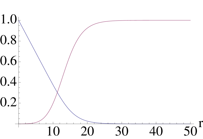
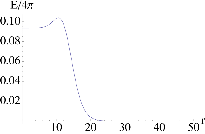
Figure 1: Field profiles for a solution with a non-vanishing magnetic charge and corresponding energy density. The red line corresponds to $k(r)$ whilst the blue line to the Higgs field $\psi(r)$. The plots correspond to the numerical values (in appropriate units of $v$) $R_{0}=4$, $\lambda=0$, $L=50$.

Now let us solve for the case in which $\lambda\neq 0$, then we choose

$$\psi(0)=0,\quad\psi(L)=1$$ (39)

$$k(0)=1,\quad k(L)=0,$$ (40)

for which the magnetic charge $|Q|=1$. Solutions are shown in figures 2 and 3. Here we see that as we expected the energy density tends to a constant at large $r$ which indicates that the solutions need to be regulated in the IR. There is also a well defined core radius close to $r=0$. Our set up has a natural regulator in a finite size tube $L$. Interestingly we see that there is a large region where the energy density grows linearly with $L$. Raising $\lambda$, thus raising the Higgs mass narrows the core of the solution. Conversely, making the cross-section of the tube smaller by decreasing $R_{0}$ increases the size of the core. In figure 3 we show the solution corresponding to picking boundary conditions such as to pick out the other vacuum at small $R_{0}$. In this case we find a much narrower core and a correspondingly higher energy density there. Figure 4 shows a different solution to the same equations in which we set $R_{0}=\sqrt{2}/\lambda$ with $\lambda=1$, this point is of special importance as for this choice of $\lambda$ the two vacua in which $k=0,\;\psi=1$ and $k=1,\;\psi=0$ are degenerate. As shown in the next section this point is of further importance in the context of solving equations (14)-(15) analytically. Once again, the solution requires a IR regulator. As expected these solutions can be traced to trajectories in the Newtonian potential. Figure 5 shows $-V(x,y)$ for both the parameters used in the solutions shown in figures 2 and 3, we see that these solutions correspond to trajectories in which, in the first case, one starts at the maximum of the potential and tends towards the minimum (dark red area). Figure 6 shows the potential which represents the solution shown in figure 4 interpolating between two degenerate minima. These solutions correspond to the parameters $c_{1}$ and $c_{2}$ found using equations (20) and (21).

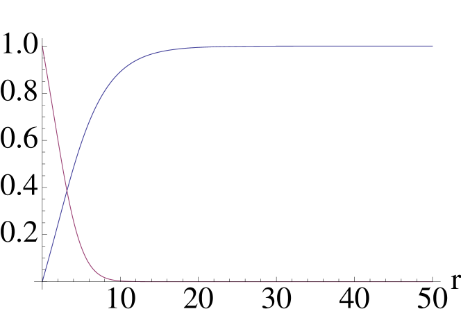
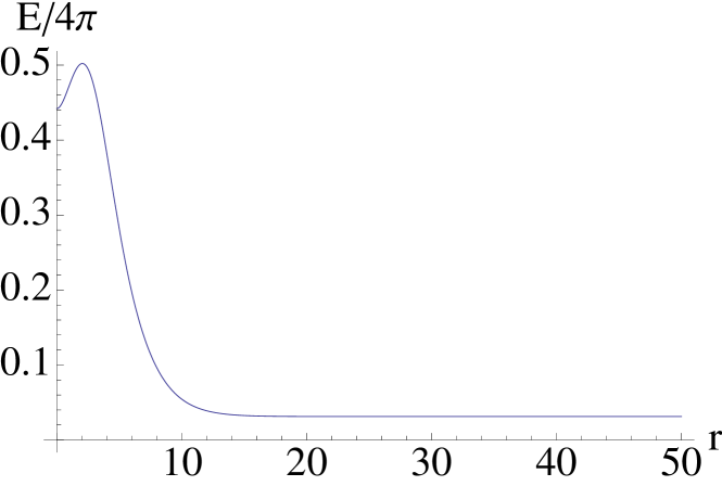
Figure 2: Field profiles for a solution with a non-vanishing magnetic charge and corresponding energy density. The red line corresponds to $k(r)$ whilst the blue line to the Higgs field $\psi(r)$. The plots correspond to the numerical values (in appropriate units of $v$) $R_{0}=4$, $\lambda=0.3$, $L=50$.

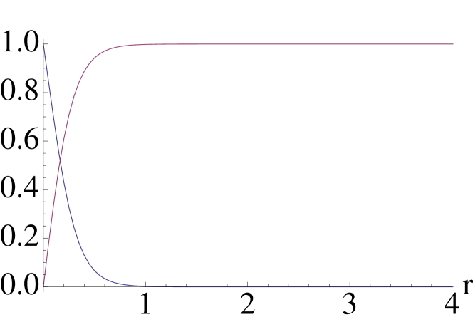
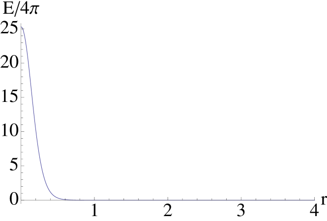
Figure 3: Field profiles for a solution with a non-vanishing magnetic charge and corresponding energy density. The red line corresponds to $k(r)$ whilst the blue line to the Higgs field $\psi(r)$. The plots correspond to the numerical values (in appropriate units of $v$) $R_{0}=0.2$, $\lambda=0.5$, $L=50$. The energy tends to a small non-zero constant.

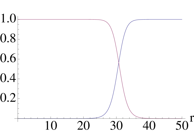
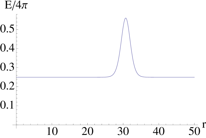
Figure 4: Field profiles for a solution with a non-vanishing magnetic charge and corresponding energy density. The red line corresponds to $k(r)$ whilst the blue line to the Higgs field $\psi(r)$. The plots correspond to the numerical values (in appropriate units of $v$) $R_{0}=\sqrt{2}/\lambda$, $\lambda=1$, $L=50$.

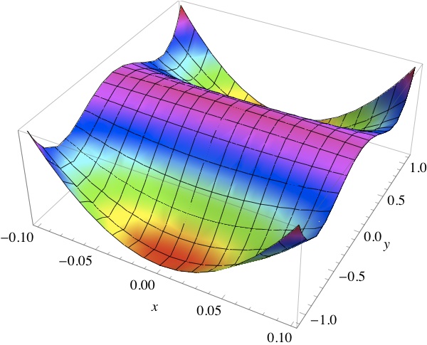
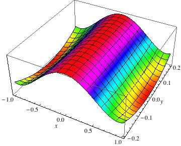
Figure 5: Potential profiles corresponding to the parameters chosen for solutions in figures 2 and 3 respectively. The darker red regions correspond to minima of the potential. In both cases the solutions can be traced to trajectories in the Newtonian potential.

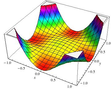
Figure 6: Potential profiles corresponding to the parameters chosen for the solution shown in figure 4. The darker red regions correspond to minima of the potential. In this special point the solution interpolates between two minima of the effective potential.

3.3 The special point

Remarkably enough, for a particular choice of $R_{0}$ the system of eqs (14) and (15) admits (in the case of non-vanishing Higgs coupling) a direct analytic treatment in terms of elliptic integrals. Let us consider the case in which

$$R_{0}=\frac{\sqrt{2}}{\lambda}\ .$$ (41)

In this case, with the ansatz

$$\psi=bk\ ,$$ (42)

where

$$b^{2}=\frac{\lambda^{2}}{\lambda^{2}-2}\ ,\ \ \frac{\lambda^{2}}{2}>1\ ,$$ (43)

the system of equations (14) and (15) reduces to the single differential equation

$$k^{\prime\prime}-k^{3}\left(b^{2}+\frac{\lambda^{2}}{2}\right)+\frac{\lambda^{2}}{2}k=0,$$ (44)

which may be integrated to give

$$I+\frac{k^{4}}{4}\left(b^{2}+\frac{\lambda^{2}}{2}\right)-\frac{\lambda^{2}}{4}k^{2}=\frac{\left(k^{\prime}\right)^{2}}{2}\ ,$$ (45)

where $I$ is an integration constant. The general form of equation (44) admits kink solutions. However these solutions cannot be interpreted as magnetic monopoles because their magnetic charge vanishes. Equation (45) can be further integrated directly in terms of an elliptic function

$$\int_{k(0)}^{k(r)}\frac{dk}{\sqrt{2\left[I+\frac{k^{4}}{4}\left(b^{2}+\frac{\lambda^{2}}{2}\right)-\frac{\lambda^{2}}{4}k^{2}\right]}}=r\ ,$$ (46)

which fixes the integration constant $I$ by the following relation:

$$\int_{k(0)}^{k(L)}\frac{dk}{\sqrt{2\left[I+\frac{k^{4}}{4}\left(b^{2}+\frac{\lambda^{2}}{2}\right)-\frac{\lambda^{2}}{4}k^{2}\right]}}=L\ .$$ (47)

The above equation determines how the integration constant $I$ depends on the length of the tube $L$ once the boundary conditions on $k$ are specified. In particular, solutions corresponding to very large longitudinal length (when, formally, $L$ approaches infinity) are found by choosing the integration constant $I$ in such a way that $k(L)$ is a double pole of the denominator in eq. (47). One can also pick the integration constant in order to complete the square inside the denominator. Then for

$$I=\frac{\lambda^{4}}{16(b^{2}+\lambda^{2}/2)}$$ (48)

the integral in eq. (46), once inverted, gives

$$k(r)=a\tanh\left(-\frac{\lambda(r+C)}{2\sqrt{2}}\right),$$ (49)

where $C$ is another integration constant which one recognizes as the usual constant determining the kink centre position for this solution and $a=\sqrt{\frac{\lambda^{2}}{2(b^{2}+\lambda^{2}/2)}}$. At this special point and using the ansatz in eq. (42) the energy reduces to

$$E=2\pi\lambda^{2}\int_{0}^{L}\left[\frac{(\lambda^{2}+1)}{2\lambda^{2}}-\left(\frac{\lambda^{2}-1}{\lambda^{2}-2}\right)k^{2}+\frac{1}{2}\left(\frac{\lambda^{4}+\lambda^{2}-4}{(\lambda^{2}-2)^{2}}\right)k^{4}+\frac{2}{\lambda^{2}}\left(\frac{\lambda^{2}-1}{\lambda^{2}-2}\right)k^{\prime 2}\right]dr,$$ (50)

which admits a standard completion in terms of a boundary term plus a constant. The boundary term is simply related to the boundary values of the kink profile $k(r)$ whilst the constant is responsible for the linear dependence of the energy on the length of the tube $L$, as expected from the arguments presented in the previous section.

3.3.1 Long-Lived breathers

One of the most interesting phenomena which occurs in soliton theory in $1+1$ dimensions is the existence of long-lived breathers (two detailed reviews are [17] [18]). Breathers are long lived oscillating lumps which lose energy by emitting small amplitude waves. For small enough amplitudes, the energy emission rate is so slow that it cannot be detected by a numerical computation. This intriguing phenomenon at first glance appears to be quite specific to $1+1$ dimensions since it is known that, in $3+1$ dimensions breathers have short lifetimes. Hence, one could think that in the case of the hedgehog sector of the Yang-Mills-Higgs system (which is intrinsically $3+1$ dimensional due to the hedgehog ansatz) one should not be able to find long-lived breathers. In fact, another benefit of the present geometry is that it allows one to find such long-lives breathers, as we will shortly show.

To see this, let us generalize the ansatz eq.(11) to include time-dependence in the form

$$A_{\mu}=\left(k\left(t,r\right)-1\right)U^{-1}\partial_{\mu}U\ ,\ \ \Psi=\psi(t,r)U\ ,$$ (51)

where $U$ is defined as before in eqs. (12) and (13). In this case, the system’s equations of motion in the background metric of eq. (4) reduce to

$$\left(\frac{\partial^{2}}{\partial r^{2}}-\frac{\partial^{2}}{\partial t^{2}}\right)\psi-2\frac{k^{2}\psi}{\left(R_{0}\right)^{2}}+\frac{\lambda^{2}}{2}\psi\left(1-\psi^{2}\right) =0\ ,$$ (52)

$$\left(\frac{\partial^{2}}{\partial r^{2}}-\frac{\partial^{2}}{\partial t^{2}}\right)k+\frac{k\left(1-k^{2}\right)}{\left(R_{0}\right)^{2}}-k\psi^{2} =0\ .$$ (53)

Interestingly enough, for the particular case in which $R_{0}$ is chosen as in eq. (41) the above system reduces to the following single scalar PDE:

$$\left(\frac{\partial^{2}}{\partial r^{2}}-\frac{\partial^{2}}{\partial t^{2}}\right)k-k^{3}\left(b^{2}+\frac{\lambda^{2}}{2}\right)+\frac{\lambda^{2}}{2}k=0\ .$$ (54)

The key observation is that eq. (54) (together with the corresponding expression for the energy-density) coincides with the equation for a field theory in $1+1$ dimensions with cuartic interactions (along with the energy-density), which is known to have long-lived breather solutions [17] [18]. Hence, the Yang-Mills-Higgs system in the geometry described by the metric in eq. (4) admits breather solutions which remain in an oscillatory state for a long time, with minimal emission of radiation (for a detailed numerical analysis see [19]).

4 Dyonic solutions

The present framework allows the inclusion of static dyonic solutions. Let us consider the following ansatz for the gauge and Higgs fields

$$A_{0}=\sqrt{2}F(r)U,\ \ A_{i}=\left(k\left(r\right)-1\right)U^{-1}\partial_{i}U\ ,\ \ \Psi=\psi(r)U\ ,$$ (55)

where $U$ is defined in eqs. (12) and (13) and $i=1,2,3$ and the factor of $\sqrt{2}$ in $A_{0}$ is added for notational convenience. The non-abelian magnetic and electric charges are

$$Q_{M}=4\pi\int_{0}^{L}\frac{\partial}{\partial r}\left[\psi\left(k^{2}-1\right)\right]dr,$$ (56)

$$Q_{E}=4\pi R_{0}^{2}\int_{0}^{L}\frac{\partial}{\partial r}\left[\psi F^{\prime}\right]dr.$$ (57)

In the tube-shaped domain described by eq. (4) the Yang-Mills-Higgs equations of motion reduce to

$$\psi^{\prime\prime} =2\frac{k^{2}\psi}{\left(R_{0}\right)^{2}}-\frac{\lambda^{2}}{2}\psi\left(1-\psi^{2}\right)\ ,$$ (58)

$$k^{\prime\prime} =-\frac{k\left(1-k^{2}\right)}{\left(R_{0}\right)^{2}}+k\psi^{2}-kF^{2}\ ,$$ (59)

$$F^{\prime\prime} =\frac{2Fk^{2}}{\left(R_{0}\right)^{2}}\ .$$ (60)

Unfortunately, in the dyonic case, the above system of equations cannot be mapped into a three-dimensional effective mechanical problem with a conservative potential. However, one again one can see that the present framework brings a very useful simplication. Namely, despite the fact that the mechanical analogy is unavailable, still, the system in eqs. (58), (59) and (60) is autonomous (since no explicit power of the independent $r$ appears) and so the theory of dynamical systems can be applied to study the asymptotic qualitative behavior of the above solutions.

The energy of the system becomes

$$E=\frac{4\pi}{R_{0}^{2}}\int_{0}^{L}\left[\frac{1}{2}\left(1+k^{4}\right)+k^{2}\left(R_{0}^{2}(\psi^{2}+F^{2})-1\right)+\frac{\lambda^{2}}{8}R_{0}^{4}(1-\psi^{2})^{2}+R_{0}^{2}k^{\prime 2}+\frac{1}{2}R_{0}^{4}F^{\prime 2}+\frac{1}{2}R_{0}^{4}\psi^{\prime 2}\right]dr.$$ (61)

Once again the dyonic system is simpler than the flat-space one (see, for instance, [14]) due to the fact that in eqs. (58), (59) and (60) no explicit power of the radius $r$ appears (neither, of course, do the angular coordinates thanks to the hedgehog property). The vacuum structure follows similarly to the purely magnetic case. Clearly, the real vacuum at $\lambda=0$ will have $F=0$. When $\lambda\neq 0$ then the minimal energy density is achieved when $F=c$, where $c$ is a constant. Equation (60) also admits a solution in which $F(r)$ is linear in $r$ when $k=0$.

4.1 The BPS solutions

The BPS equations (9) corresponding to $\lambda=0$ reduce to

$$\partial_{r}k-\sin(\alpha)k\psi=0,$$ (62)

$$\sin({\alpha})\partial_{r}\psi+\frac{1-k^{2}}{R_{0}^{2}}=0,$$ (63)

$$F=\cos(\alpha)\psi.$$ (64)

The general solution of the system reads

$$k=\exp u\ ,$$ (65)

$$\sin(\alpha)\psi=\partial_{r}u\ ,\ \ F=\cos(\alpha)\psi\ ,$$ (66)

where, as in the purely magnetic case, the function $u(r)$ is given by the inverse of the integral in eq.(26).

4.2 Numerical Solutions

Let us proceed to solve equations (58)-(60) numerically. A dyon solution will be a solution which at large $L$ tends to the real vacuum and has non-vanishing electric and magnetic fields. In the case of vanishing $\lambda=0$ we can further simplify the equations by using an ansatz where $F=\psi$, then we seek solutions with boundary conditions

$$\psi(0)=1,\quad\psi(L)=0$$ (67)

$$k(0)=0,\quad k(L)=1.$$ (68)

Figure 3 shows such a solution corresponding to a well localized dyon. This solution is valid for any $L$ extending out to infinity. The effect of decreasing $R_{0}$ is to make the core size of the dyon smaller. Then the BPS charges are

$$Q_{M}=4\pi,\quad Q_{E}\approx-4\pi(1.232)$$ (69)

and numerically we find that

$$\frac{E_{dyon}}{4\pi}=1.704>\frac{1}{4\pi}\sqrt{Q_{M}^{2}+Q_{E}^{2}}=1.587.$$ (70)

Therefore we conclude that, even for $\lambda=0$ this solution is not BPS saturated. This is to be expected, not every solution of equations (58)-(60) is also a solution of (62)-(64) (the inverse statement however is true). Specifically for our solution $F=\psi$ which corresponds to $\alpha=0+2\pi n$ in equation (64). Then this is only a solution of the full set of BPS equations if $k=1$ identically, which is clearly not the case of our numerical solution.

Let us switch on a potential and set $\lambda\neq 0$. Then we seek solutions where

$$\psi(0)=0,\quad\psi(L)=1$$ (71)

$$k(0)=1,\quad k(L)=0.$$ (72)

$$F(0)=1,\quad F^{\prime}(L)=0.$$ (73)

A solution satisfying these boundary conditions is shown in figure 8. As expected this solution has non-vanishing energy density at large $r$ where it tends to a constant $E=4\pi/R_{0}^{2}$. Once again, the energy in this region will be proportional to the tube length $L$, which serves as the IR regulator. Increasing $\lambda$ decreases the size of the core whilst increasing $R_{0}$ makes the asymptotic value of $F\rightarrow\psi$ and decreases the asymptotic value of the energy whilst increasing its “core”, see figure 9. As expected, in the flat space limit the energy density should vanish at infinity.

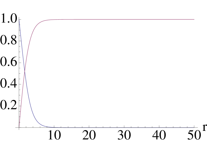
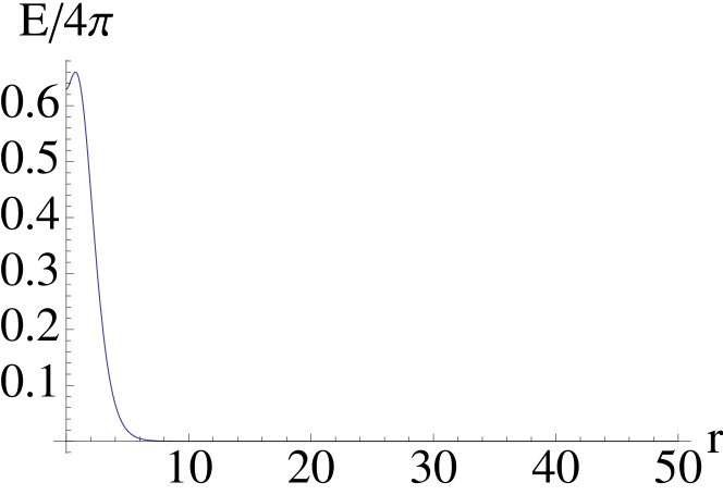
Figure 7: Field profiles for dyon solution. The red line corresponds to $k(r)$ whilst the blue line to the Higgs and electric component of the gauge fields $\psi(r)=F(r)$. The plots correspond to the numerical values (in appropriate units of $v$) $R_{0}=2$, $\lambda=0$, $L=50$.

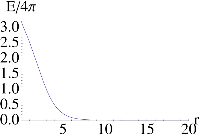
Figure 8: Field profiles for non localised dyon solution and corresponding energy density. The red line corresponds to $k(r)$, the blue line to the Higgs field $\psi(r)$ and the black like to $F(r)$. The plots correspond to the numerical values (in appropriate units of $v$) $R_{0}=5$, $\lambda=0.5$, $L=50$.

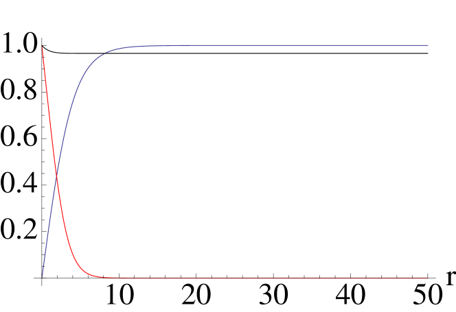
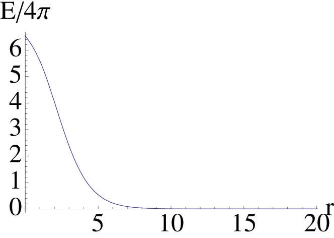
Figure 9: Field profiles for non localised dyon solution and corresponding energy density. The red line corresponds to $k(r)$, the blue line to the Higgs field $\psi(r)$ and the black like to $F(r)$. The plots correspond to the numerical values (in appropriate units of $v$) $R_{0}=8$, $\lambda=0.5$, $L=50$.

5 Conclusions

We considered exact and numerical solutions of the four-dimensional Yang-Mills-Higgs system with and without the Higgs coupling $\lambda$ in the background of $\mathbb{R}\times S^{2}$. These non-Abelian magnetic configurations can live within both closed and open tubes whose sections are spherical caps admitting a smooth flat limit. When $\lambda=0$ the solutions describe magnetic monopoles with a finite energy density. When one switches on a Higgs potential, and unlike what happens in flat case, the energy of the solutions grows linearly with $L$ at large distances, which thus serves as a good cut-off. In the flat limit $R_{0}\rightarrow\infty$, these configurations approach domain-walls of the Yang-Mills-Higgs system. As $R_{0}$ shrinks this has the effect of constraining the monopole to the tubular geometry which is seen as a large plateau appearing in its energy density profile. The dramatic simplification that this geometry provides not only renders the analytic treatment of the autonomous non-linear coupled system possible but also simplifies the numerical analysis. The theory of dynamical systems (which, in the standard case, is unavailable) provides many powerful techniques which, for instance, allow study of the asymptotic behaviour as well as the stability of the solutions in a general fashion (namely, without restrictions on the parameters of the theory). When the system involves only a magnetic component of the gauge field we have shown that the equations can be treated in the language of a classical particle subject to a conservative force. If the radius of curvature of the geometry is chosen to satisfy a particular relation shown in eq.(41) then the system can be further reduced to a single PDE and its energy can be determined by solving an elliptic integral without even requiring the explicit dependence on the profile functions in terms of $r$. At this special point the solutions of the system are kink-like but cannot be interpreted as magnetic monopoles as their non-Abelian charge vanishes. For the magnetic choice of gauge function and for a special choice of the curvature radius, we have explicitly shown that the hedgehog property admits the inclusion of time dependence in the field profiles which leads to breather-like solutions which remain in an oscillatory state for a remarkably long time, with minimal emission of radiation. Finally, static dyonic configurations with an electric component can be constructed analytically and numerically and satisfy similar properties. An interesting extension to this work is to consider a similar set-up in the background of $S^{1}\times S^{2}$ where one expects to see solutions with periodic boundary conditions. This is achieved simply by identifying the points at $r=0$ and $r=L$, thus one expects similar properties observed in the $\mathbb{R}\times S^{2}$ system. We defer this investigation to future work.

Acknowledgements

This work has been funded by the Fondecyt grants 1120352 and 3140122. The Centro de Estudios Científicos (CECs) is funded by the Chilean Government through the Centers of Excellence Base Financing Program of Conicyt.

References

- [1] G. ’t Hooft, Nucl. Phys. B 79, 276 (1974).
- [2] A.M. Polyakov, Zh. Eksp. Teor. Fiz. Pis’ma. Red. 20, 430 (1974) [JETP Lett. 20, 194 (1974)].
- [3] N. Manton and P. Sutcliffe, Topological Solitons, (Cambridge University Press, Cambridge, 2007).
- [4] M. Shifman, A. Yung, Supersymmetric Solitons (Cambridge University Press, Cambridge, 2009).
- [5] B. Julia and A. Zee, Phys. Rev. D 11, 2227 (1975).
- [6] A. Vilenkin, E. P. S. Shellard, Cosmic Strings and Other Topological Defects, Cambridge University Press (2000).
- [7] E. B. Bogomolny, Sov.J.Nucl.Phys. 24 (1976) 449; Yad.Fiz. 24 (1976) 861
- [8] M.K. Prasad, C. M. Sommerfield, Phys.Rev.Lett. 35 (1975) 760.
- [9] T. T. Wu, C. N. Yang, Phys. Rev. D 12, 3843 (1975).
- [10] P. Cordero, C. Teitelboim, Ann. Phys. 100, 607-631 (1976).
- [11] E. Witten, Phys. Rev. Lett. 38, 121 (1977).
- [12] M. Shifman, “Advanced topics in quantum field theory: A lecture course,” Cambridge, UK: Univ. Pr. (2012) 622 p
- [13] D. Tong, “TASI lectures on solitons: Instantons, monopoles, vortices and kinks,” hep-th/0509216.
- [14] P. Rossi, Physics Reports 86 (1982), 317.
- [15] Dynamical Systems in Cosmology, J. Wainwright and G.F.R. Ellis, Cambridge University Press, 1997.
- [16] Y. M. Shnir, “Magnetic Monopoles”, Heidelberg: Springer (2005).
- [17] Y. S. Kivnar and B. A. Malomed, Rev. Mod. Phys. 61, 763 (1989).
- [18] S. Flach and C. R.Willis, Physics Reports 295, 181 (1998).
- [19] M. Gleiser, A. Sornborger, Phys.Rev. E62 (2000) 1368.