Support Consistency of Direct Sparse-Change Learning in Markov Networks
Abstract
We study the problem of learning sparse structure changes between two Markov networks and . Rather than fitting two Markov networks separately to two sets of data and figuring out their differences, a recent work proposed to learn changes directly via estimating the ratio between two Markov network models. In this paper, we give sufficient conditions for successful change detection with respect to the sample size , the dimension of data , and the number of changed edges . When using an unbounded density ratio model we prove that the true sparse changes can be consistently identified for and , with an exponentially decaying upper-bound on learning error. Such sample complexity can be improved to when the boundedness of the density ratio model is assumed. Our theoretical guarantee can be applied to a wide range of discrete/continuous Markov networks.
keywords:
[class=MSC]keywords:
arXiv:0000.0000 \startlocaldefs \endlocaldefs
,
and
1 Introduction
Learning changes in interactions between random variables plays an important role in many real-world applications. For example, genes may regulate each other in different ways when external conditions are changed. The number of daily flu-like symptom reports in nearby hospitals may become correlated when a major epidemic disease breaks out. EEG signals from different regions of the brain may be synchronized/desynchronized when the patient is performing different activities. Identifying such changes in interactions helps us expand our knowledge on these real-world phenomena.
In this paper, we consider the problem of learning changes between two undirected graphical models. Such a model, also known as a Markov network (MN) [10], expresses interactions via the conditional independence between random variables. Hammersley-Clifford theorem [7] states that the joint distribution of an MN can be factorized over subsets of interacted random variables and general MNs may have factors over arbitrary numbers of random variables. For simplicity, we focus on a special case, namely pairwise MNs, whose joint distribution can be factorized over only single or pairwise random variables.
The problem of learning structure of MN itself has been thoroughly investigated in the last decade. The graphical lasso method [1, 6] learns a sparse precision (inverse covariance) matrix from data by using the -norm, while the neighborhood regression methods [11, 13, 18] solve a node-wise lasso program to identify the neighborhood of each single node.
One naive approach to learning changes in MNs is to apply these methods to two MNs separately and compare the learned models. However, such a two-step approach does not work well when the MNs themselves are dense (this can happen even when the change in MNs is sparse). A recent study [32] adopts a neighbourhood selection procedure to learn sparse changes between Gaussian MNs via a fused-lasso type regularizer [24]. However, no theoretical guarantee was given on identifying changes. Furthermore, extension of the above mentioned methods to general non-Gaussian MNs is hard due to the computational intractability of the normalization term.
To cope with these problems, an novel algorithm has been proposed recently [12]. Its basic idea is to model the changes between two MNs and as the ratio between two MN density functions and , and the ratio is directly estimated in one-shot without estimating and themselves [22]. Since parameters in the density ratio model represent the parametric difference between and , sparsity constrains can be directly imposed for sparse change learning. Thus, the density-ratio approach can work well even when each MN is dense as long as the change is sparse. Furthermore, the normalization term in the density-ratio approach can be approximately computed by the straightforward sample average and thus there is no computational bottleneck in using non-Gaussian MNs. Experimentally, the density-ratio approach was demonstrated to perform well. However, its theoretical properties have not been explored yet.
The ability of recovering a sparsity pattern via a sparse learning algorithm has been studied under the name of support consistency or sparsistency [27], that is, the support of the estimated parameter converges to the true support. Previous works for successful structure recovery are available for -regularized maximum (pseudo-)likelihood estimators [18, 30]. However, density ratio estimator in [12] brought us a new question: what is the sparsistency of identifying correct sparse changes without learning individual MNs? Such a concern is very practical since in applications such as learning changes in gene expression between stimuli conditions, we only care changes rather than individual structures before or after changes. We illustrate such an example in the problem of gene regulatory networks in Section 7.
In this paper, we theoretically investigate the success of the density-ratio approach and provide sufficient conditions for successful change detection with respect to the number of samples , , data dimension , and the number of changed edges . More specifically, we prove that if and , changes between two MNs can be consistently learned under mild assumptions, regardless the sparsity of individual MNs. Such sample complexity can be further improved to when the boundedness of the density ratio model is assumed. Technically, our contribution can be regarded as an extention of support consistency of lasso-type programs [27] to the ratio of MNs. The convergence rate does not rely on the individual sparsity of each MN, thus structures like hub-nodes can exist. Such hub structure is common in many applications, such as gene expression data where one gene regulates many other genes. Our theorem holds for the most general log-linear MN models, and does not assume any special type of individual MNs (such as Gaussian or Ising).
Note that the theoretical results presented in this paper are fundamentally different from previous works on learning a “jumping MN” [9], where the focuses are learning the partition boundaries between jumps, and the successful recovery of graphical structure within each partition, rather than learning sparse changes between partitions.
In previous works [18, 30], the (upper/lower) boundedness of the Fisher information matrix, or log-partition function derivatives of a density model are often assumed. In this work, similar assumptions are imposed on the true density ratio model. Moreover, we show that such assumptions have profound links with the smoothness of our model, which implies the magnitude of change should not be too drastic for keeping the density ratio model well-behaved. These assumptions are also automatically satisfied under some special cases.
The target of [12] coincides with another recently proposed method where a differential network is learned directly using a different technique [33]. Without learning a precision matrix for each MN, this approach estimates a differential network utilizing a special equality obtained for Gaussian MNs. However, such an objective function does not generalize to ordinary pairwise MNs. The theorems obtained in this paper and the ones in [33] both rely on one similar assumption: The changes are sparse. However, theorems in this paper manage to achieve the same sample complexity of recovering the correct structure changes without explicitly assuming Gaussianity over datasets.
This paper is organized as follows: First we introduce the problem formulation of learning changes between two MNs in Section 2. Second, we review the density ratio estimation method proposed in [12]. Then, as the main focus of this paper, we analyze the sufficient conditions for successful change detection, i.e., the support consistency of such algorithm in Section 3 and 4. Moreover, in Section 5, we study the key assumptions in this paper, and discuss their consequences. Through experiments in Section 6, we demonstrate the validity of our theorems and compare the performance of the density ratio approach with a state of the art method. Finally, in Section 7, we show the density ratio method successfully identifies key changes in a gene network between two stimuli conditions.
2 Direct Change Learning between Markov Networks
In this section, we review a direct structural change detection method [12].
2.1 Problem Formulation
Consider two sets of independent samples drawn separately from two probability distributions and on :
We assume that and belong to the family of Markov networks (MNs) consisting of univariate and bivariate factors, i.e., their respective probability densities and are expressed as
| (1) |
where is the -dimensional random variable, denotes the transpose, is the -dimensional parameter vector for the elements and , and
is the entire parameter vector. is a bivariate vector-valued basis function, and is the normalization factor defined as
is defined in the same way. Using these notations, we can define two well-known MNs as examples:
Ising-model (see e.g.[10])
One of the earliest and widely known graphical models is the Ising model, where , and . For all pairs , where is the edge set of the graphical model, is a scalar and has non-zero value.
Gaussian MN
Gaussian MN is a representative of continuous MN. and . For all pairs or , is a scalar and has non-zero value.
The research problem now becomes clear: Given two parametric models and , we hope to discover changes in parameters from to , i.e., .
2.2 Density Ratio Formulation for Structural Change Detection
The key idea in [12] is to consider the ratio of and :
where encodes the difference between and for factor , i.e., is zero if there is no change in the factor .
Once the ratio of and is considered, each parameter and does not have to be estimated, but only their difference is sufficient to be estimated for change detection. Thus, in this density-ratio formulation, and are no longer modeled separately, but it models the changes from to directly as
| (2) |
where is the normalization term. This direct formulation also halves the number of parameters from both and to only .
The normalization term is chosen to fulfill :
which is the expectation over . This expectation form of the normalization term is another notable advantage of the density-ratio formulation because it can be easily approximated by the sample average over :
Thus, one can always use this empirical normalization term for any (non-Gaussian) models and .
An important observations can be made from this formulation: Although two MNs may have sophisticated models individually, their changes might be “simple” since many terms may be canceled while taking the ratio, i.e. might be zero. Thus, if we use in our ratio model, it does not mean we assume two individual MNs are Gaussian or Ising, it simply means we assume the changes of interactions are linear while other non-linear interactions remain unchanged. This formulation allows us to consider highly complicated MNs as long as their changes are “simple”. We will give a concrete example later.
Throughout the rest of the paper, we simplify the notation from to by assuming the feature functions are the same for all pairs of random variables. However, our analysis still holds if this assumption is violated. Next, we study the density ratio formulation in the case of Gaussian MNs.
Gaussian MN
: Given two -dimensional zero-mean Gaussian MNs and parameterized by the precision matrix and respectively, it is reasonable to parametrize a density ratio model
| (3) |
where is a symmetric real-valued matrix and
However, this formulation brings a problem: it still contains an unknown parameter , meaning that we will have to learn first before we can model the difference between two MNs. To solve this problem, one may use the empirical version of the normalization term instead
| (4) |
Interestingly, by using this model, the Gaussianity assumption has been loosened: the normalization term is obtained by an empirical average and did not use the analytical form offered by the Gaussianity of . Thus, it can actually model the density ratio for any and as long as their changes are limited to the quadratic components.
2.3 Direct Density-Ratio Estimation
Density ratio estimation has been recently introduced to the machine learning community and is proven to be useful in a wide range of applications [22]. In [12], a density ratio estimator called the Kullback-Leibler importance estimation procedure (KLIEP) for log-linear models [21, 26] was employed in learning structural changes.
For a density ratio model , the KLIEP method minimizes the Kullback-Leibler divergence from to :
| (5) |
Note that the density-ratio model (2) automatically satisfies the non-negativity and normalization constraints:
Here we define
as the empirical density ratio model. In practice, one minimizes the negative empirical approximation of the rightmost term in Eq.(5):
Because is convex with respect to , its global minimizer can be numerically found by standard optimization techniques such as gradient descent or quasi-Newton methods. The gradient of with respect to is given by
| (6) |
that can be computed in a straightforward manner for any feature vector .
Importance Sampling
From the gradient of KLIEP (6), we can observe a clear link between KLIEP and Importance Sampling (see e.g., [19]). The second term on the right-hand side is an “importance sampled” approximation of using our density ratio model while the first term is a straightforward sample average. The population version of (6) equals zero if and only if . Therefore, one should aware that the assignment of and may affect the performance of such an approximation as importance sampling can be easily affected by the choice of the instrumental distribution (in this case, ). To reduce the estimation variance, is usually picked as the one with a thicker tail [28]. This observation reveals a fundamental asymmetry of KLIEP which will be discussed in Section 8.
Gaussian MN
2.4 Sparsity-Inducing Norm
To find a sparse change between and , one may regularize the KLIEP solution with a sparsity-inducing norm , i.e., the group-lasso penalty [31] where we use to denote the norm. Note that the separate density estimation approaches sparsify both and so that the difference is also sparsified. On the other hand, the density-ratio approach [12] directly sparsifies the difference , and thus intuitively this method can still work well even if and are dense as long as is sparse.
Now we have reached our final objective:
| (8) |
3 Support Consistency of Direct Sparse-Change Detection
The above density-ratio approach to change detection was demonstrated to be promising in empirical studies [12]. However, its theoretical properties have not yet been investigated. In this section, we give theoretical guarantees of the convex program (8) on sparse structural change learning. More specifically, we give sufficient conditions for detecting correct changes in terms of the sample size and , data dimensions , and the number of changed edges , followed by the discussion of the insights we can gain from such theoretical analysis.
3.1 Notations
In the previous section, a sub-vector of indexed by corresponds to a specific edge of an MN. From now on, we use new indices with respect to the “oracle” sparsity pattern of the true parameter for notational simplicity. We introduce the “true parameter” notation and the pairwise index set . Two sets of sub-vector indices regarding to and are defined as We rewrite the objective (8) as
| (9) |
Similarly we can define and accordingly. Sample Fisher information matrix denotes the Hessian of the log-likelihood: where we simplify as . is a sub-matrix of indexed by two sets of indices on rows and columns.
We also concatenate to get a “linearized” version of the feature function as
and is the partial output of indexed by a set of indices .
Gaussian MN
Here we derive the Fisher information matrix for the Gaussian MN ratio model. Define an auxiliary matrix :
where . The Fisher information matrix of the likelihood function using the Gaussian density ratio model described in (7) has the form
3.2 Assumptions
There is an important guideline for imposing assumptions in this paper: we try not to put any explicit constrains on the types of individual MN or nor their structures, but only on the changes between them. This is crucial since KLIEP is a direct and flexible change learning method and have no restrictions on the types of individual MNs on which it works. Therefore, we hope to obtain the most generic theorem for this method.
Similarly to previous researches on sparsity recovery analysis [27, 18], the first two assumptions are made on the Fisher information matrix.
Assumption 1 (Dependency Assumption).
The sample Fisher information submatrix has bounded eigenvalues:
with probability 1, where is the minimum-eigenvalue operator of a symmetric matrix
This assumption on the submatrix of is to ensure that the model is identifiable (see B.1 in Appendix for details). Note “” denotes either eigenvalue or regularization parameter depending on its subscript.
Assumption 2 (Incoherence Assumption).
with probability 1, where .
This assumption says the unchanged edges cannot exert overly strong effects on changed edges and is a common assumption can be found in previous literatures on support consistency analysis such as [27, 18].
Assumption 3 (Smoothness Assumption on Likelihood Ratio).
The log-likelihood ratio is smooth around its optimal value, i.e., it has bounded derivatives
| (10) | ||||
| (11) | ||||
with probability .
, are the spectral norms of a matrix and a tensor respectively (See e.g., [25] for the definition of spectral norm of a tensor). Note that (10) also implies the bounded largest eigenvalue of . Assumption 3 can be regarded as an analogy of assumptions on the log-normalization function in [30]. As we set no explicit restrictions on the type of distribution and , this assumption guarantees the log-likelihood function is well-behaved.
Now, we make the following assumptions on the density ratio:
Assumption 4 (The Correct Model Assumption).
The density ratio model is correct, i.e. there exists such that
Assumptions 1, 2, and 3 are in fact related to distribution . However, the density ratio estimation objective is an M-estimator summed up over samples from . Assumption 4 provides a transform between and and allows us to perform analysis on such an M-estimator in an “importance sampling” fashion.
Next, we impose assumptions on the “smoothness” of the density ratio model. Generally speaking, if we expect good performance from the density ratio estimator, the density ratio model should be “well-behaved”. The following assumption quantifies such an intuition.
Assumption 5 (Smooth Density Ratio Model Assumption).
For any vector such that and every , the following inequality holds:
We list a few consequences of the Assumption 5.
Proposition 1.
For all and for any vector such that ,
Using Assumption 5, we get Proposition 1 that provides a tail probability bound of the density ratio model on , which is further used to obtain an exponentially decaying upper-bound of empirical approximation error of the log-normalization term (see Proposition 12 in Appendix for details).
Proposition 2.
For any vector such that ,
Proof.
Noting , the above inequalities is the consequence of sub-Gaussianity. ∎
Since the density ratio can be thought as the magnitude of change between two MNs, Proposition 2 tells the fact that the change should not be too drastic in order to keep our ratio-model well-behaved.
We are now ready to state the main theorem.
3.3 Sufficient Conditions for Successful Change Detection
The following theorem establishes sufficient conditions of change detection in terms of parameter sparsity. Its proof is provided in Section 4.1. First, let us define (see Figure 10 in Appendix for its plot) which is smaller than 1 when .
Theorem 1.
Suppose that Assumptions 1, 2, 3, 4, and 5 as well as are satisfied, where is the number of changed edges defined as , i.e., the cardinality of the set of non-zero parameter groups. Suppose also that the regularization parameter is chosen so that
| (12) |
where , and is a positive constant. Then there exist some constants , , and such that if , with the probability at least
| (13) |
the following properties hold:
-
•
Unique Solution: The solution of (9) is unique.
-
•
Successful Change Detection: and , where and are estimated sparse/non-sparse indices.
First, it is interesting to analyze the sample complexity of , which is a novel element in this research. Intuitively, one should obtain a sufficient number of samples from to accurately approximate the normalization term. Theorem 1 states should grow at least quadratically with respect to , which is undesirable if is large. In the next corollary, we discuss a relaxed coupling between and with some extra but mild cost.
Second, Assumption 5 together with Proposition 2 shows the variation allowed for the density ratio model is irrelevant to the number of changed edges . This implies that, if is large, we are only able to detect weak changes that do not cause huge fluctuations in the density ratio model, which is rather restrictive and unrealistic in some occasions, since the magnitude of change usually increases when the number of changed edges increases. Below, we consider another more relaxed scenario, where the assumption on the smoothness of the density ratio model is allowed to grow with .
Assumption 6.
For any vector such that and every , the following inequality holds:
where is the number of changed edges.
Proposition 3.
For some small constants and any vector such that , then
Proposition 4.
For any vector such that ,
From Proposition 4 we can see the magnitude of changes between MNs are allowed to grow at most linearly with . Now we see how much this will bring changes to our sufficient conditions:
Corollary 1.
See Appendix B.6 for the proof. Corollary 1 states that it is possible to drop the growth rate of on from 2 to 1 with the cost that has to grow with (rather than just in the previous case). This is an encouraging result, since with slight changes on growth rate with respect to and , we are able to consider a milder coupling between and .
Moreover, under the weaker Assumption 6, now grows linearly with . It shows the prices we need to pay when consider the magnitude of changes increasing with .
So far, we have only considered the scaling quadruple . However, it is also interesting to consider that the scalability of our theorem relative to , the dimension of the pairwise feature vector. This is a realistic scenario: It may be difficult to know the true underlying model of MN in practice, and thus we may adopt a model that contains many features to be “flexible enough” to describe the interactions among data. In the following corollary, we restate Theorem 1 with and a new scalar , which is the maximum number of non-zero elements in a pairwise feature vector . We assume that the positions of non-zero elements are independent of each sample .
Corollary 2.
3.4 Discussions
From the above theorem, one may gather some interesting insights into change detection based on density ratio estimation.
First, the required number of samples depends solely on and and is irrelevant to the number of edges of each MN. In contrast, separate graphical structural learning methods require more samples when each MN gets denser in terms of the number of edges or neighborhood [13, 18, 17]. This establishes the superiority of the density-ratio approach in sparse change detection between dense MNs. In other words, in order to detect sparse changes, the density-ratio approach does not require the individual MN to be sparse.
Second, the growth of is also lower-bounded and grows quadratically with respect to . This result illustrates the consequence of introducing a sample approximated normalization term . An insufficient number of samples from would lead to poor approximation of the normalization term, and makes change detection more difficult. Fortunately, such growth rate can be further relaxed, and with slightly increased sample complexity of .
Finally, our theorem also points out the limits of the density-ratio approach. Our analysis shows that the density ratio model may not deviate too much from its mean over distribution . A previous study on another density ratio estimator also has a similar observation [29]. Since the density ratio indicates how much differs from , this analysis generally implies that to make KLIEP work, the discrepancy between and should be mild. This is a reasonable assumption since we have already assumed that the changes in the MN structure are sparse. In high dimensional setting, it implies and are similar. Similar assumption can be found in [33] where the -1 norm of the differences between two precision matrices is bounded.
4 Proof of Support Consistency
4.1 The Proof Outline of the Main Theorem
The procedure of the main proof partially follows the steps of previous support consistency proofs using the primal-dual witness method [27], however, the problem settings are quite different: First, is a likelihood ratio between two densities which means that two sets of samples are involved in this proof and we have to consider the sparsity recovery conditions not only on one dataset, but with respect to two different MNs. Second, we did not explicitly limit the types of distribution for and , and the parameter of each factor is a vector rather than a scalar, which gives enough freedom for modelling highly complicated distributions. To the best of our knowledge, this is the first sparsity recovery analysis on learning changes between two type-free MNs. From now on, is shortened as .
First, define a dual variable associated with using the following equality:
| (14) |
and if is the subgradient of , i.e., , (14) is the optimality condition of (9) and is an optimal solution to (9). Moreover, the next Lemma tells the relationship between dual variable and sparsity patterns of any other optimal solution of (9).
Lemma 1.
See Appendix B.1 for the proof.
Now we illustrate the proof procedure of Theorem 1:
-
•
Solve the constrained optimization problem
(15) -
•
For all , set , and let ;
-
•
Obtain for all using equality (14);
- •
Bounding requires obtaining from (14). More specifically, from (14) we have:
Applying Mean-value Theorem,
| (16) |
where is between and in a coordinate fashion. We can then rewrite (16) in block-wise fashion:
| (17) |
Substitute into (4.1), we have
Rearrange terms, we have
According to triangle inequality,
By assumption, , and we obtain
Now we need to show the boundedness of and .
The boundedness of , which is the gradient of log-likelihood function on , is guaranteed by the following lemma:
Lemma 2.
There exist constants and and if the regularization parameter satisfies
then
| (18) |
Quite different from similar lemmas in previous works (such as Lemma 2 in [18]), Lemma 2 is not a simple concentration of sample mean converging to its population mean, since the gradient of the likelihood contains two sets of data from different distributions and . Moreover, the sub-Gaussianity or the boundedness of the of or were not assumed, so the concentration inequality cannot be applied here. Instead, via the smoothness behavior of the likelihood ratio function (Assumption 3), we are able to derive such a boundedness of without using any explicit properties of two distributions.
The consequence of such differences is important: this analysis allows us to consider a very wide range of distributions which may not be well-behaved (e.g. heavy-tailed), as long as the change between two distributions are minor. After all, all assumptions are imposed on the density ratio model only, rather than or . This analysis preserves the flexibility of the density ratio estimation methodology. The proof of Lemma 2 can be found in Appendix B.2.
The next lemma bounds the difference between the estimated parameter and the true parameter over the non-sparse indices, which is further used to bound and derive the sample complexity.
Lemma 3.
If and then ,
The boundedness of is finally given by
Lemma 4.
If and , then .
To show the correct non-zero pattern recovery, it suffices to show
Since Lemma 3 shows we just need to ensure such recovery.
4.2 Sample Complexity
The sample complexity for and are derived from the conditions of the Lemmas. To make Lemma 2 holds, we may set where is chosen so that the lower bound of in the Lemma 2 is satisfied. Since the upper-bound is a constant while such setting of is always decaying as grows, it is automatically satisfied at some point.
Moreover, should also satisfy the upper-bound condition in Lemma 4: and this inequality can be satisfied when .
5 Analysis of Assumptions
In this section, we investigate the conditions under which the maximum (minimum) eigenvalues of likelihood ratio derivatives are bounded. We show that under mild regularity conditions of sample statistics of distribution and tightened smoothness conditions of the density ratio model, Assumption 1 and 3 holds automatically.
5.1 Bounded Density Ratio Model
Since the derivatives of the log-likelihood ratio expresses the curvature of our objective function, we expect the smoothness of the density ratio model may play an important role in such analysis. To begin with, consider a simple bounded-ratio model by replacing the smoothness Assumption 5 (or 6) with a tightened Assumption 7:
Assumption 7 (Smooth Density Ratio Model Assumption).
For any vector such that , the following inequality holds:
As consequences, and , where and are all constants.
Since Assumption 7 is stronger than Assumption 5 or 6 (for appropriately chosen and ), the proof of Theorem 1 still holds if one uses above assumptions to substitute Assumption 5 or 6. However, as we will demonstrate later, an improved sample complexity for can be derived.
As Assumption 1 and 3 are constructed using samples from distribution , it is also natural to assume some basic regularity conditions on sample statistics:
Assumption 8 (Bounded Moments).
The feature transform , where is drawn from , has upper-bounded moments with probability one: i.e.
and
| (19) |
is bounded with probability .
is the sample covariance estimator and is the empirical expectation over samples drawn from . From now on, we remove subscript or from a random sample when summing up, as long as the indices give enough context for telling in which distribution the sample is drawn. For example, is a summation over samples drawn from distribution .
Of course, one may impose similar bounded moments constrains on the corresponding population quantities, then the above assumption automatically holds with high probability under certain regularity conditions. To avoid lengthy proofs, we stick to assumptions using sample quantities in this paper.
The following propositions show Assumptions 7 and 8 guarantee the boundedness of the derivatives of the likelihood ratio function.
Proposition 5 (Bounded Hessian).
Proposition 6 (Bounded 3rd-order Derivative).
Proposition 7 (Eigenvalue Lower Bound of Invertible Hessian Submatrix).
5.2 Sufficient Conditions under Bounded Density Ratio
Now, we give a variation of Theorem 1 based on the totally bounded density ratio model. Consider the objective
which is identical to (9) but the regularization parameter is now determined with respect to both and .
Corollary 3.
Suppose that Assumptions 2, 4, 7 and 8 as well as are satisfied. Suppose also that the regularization parameter is chosen so that
where is a positive constant. Then there exist some constants and such that if , with the probability at least , KLIEP has the same properties as those stated in Theorem 1.
Lemma 5.
If , then
where and are some constants.
5.3 Smoothness Assumption Relaxed
In the previous derivation, the assumption of boundedness of density ratio model guarantees its empirical counterpart is always upper-bounded by and is lower bounded by , but this was somewhat restrictive. In this section, we discuss a relaxation of Assumption 7 as follows:
Assumption 9 (Smooth Density Ratio Model Assumption).
For any vector such that , the following inequality holds:
| , | ||||
| (20) |
where is a constant.
Now the strictly positive lower-bound of the density ratio model is removed, and we add a new uniform lower-bound on the expectation of density ratio model around the true model. Such condition allows us to control the tail of the empirical density ratio model so that the ratio model of a specific sample from , i.e., , would not deviate “too much” from .
Note that since smoothness Assumption 9 is still stronger than 5 or 6, the proof of Theorem 1 can be used without modification to show the support consistency when this assumption is substituted. However, the proof of Corollary 3 cannot be used when Assumption 9 is imposed, since the proof requires the boundedness of which is not implied by this assumption. From now on, we show that such relaxed regime together with moment-bounding Assumption 8 also allow us to bound eigenvalues of derivatives of the likelihood function.
First, we give an example showing that if the expectation of the density ratio derivative is bounded over , the above assumption holds.
Proposition 8.
If then (20) holds.
The proof is listed in B.10 of Appendix. This proposition intuitively shows that as long as the density ratio model is smooth in the first-order, and the changes in parameter is not too drastic, our new assumption holds.
Bounding and
It can be seen from Propositions 5 and 6 that upper-bounding the second or the third order derivative relies on the upper-bound of the empirical density ratio model . However, under this new assumption, the empirical density ratio model is no longer explicitly bounded. Now we derive the upper-boundedness of using the new assumption.
Proposition 9 (Uniformly Upper-bounded ).
Bounding Minimum Eigenvalue of
Under Assumption 9, the lower-bound of empirical density ratio model is no longer valid since the density ratio can approach to 0. Here we illustrate another proof showing the boundedness of the minimum eigenvalue using concentration inequalities.
Proposition 10.
Proposition 11.
If Assumption 9 holds and the importance-sampled covariance using true density ratio model satisfies
with probability , then holds with probability at least .
5.4 Bounded Density Ratio Assumption: How Strong Is It?
In this section, we have considered a few stronger alternative assumptions to Assumptions 5 and 6 in order to derive the boundedness of derivatives of the likelihood function, which are crucial to the proof of Theorem 1. However, it is natural to ask, how strong these assumptions are?
The main advantage of the density ratio based change detection described in [12] is that such a method does not limit itself to certain distributions. Therefore, limiting the differences between two distributions help us avoid making assumptions on individual MNs.
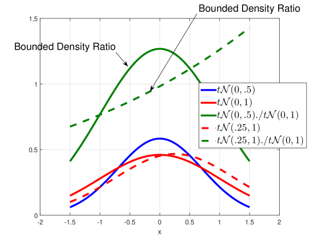
In fact, the totally bounded density ratio assumption (Assumption 7) is very well justified through our “interest”: learning the changes between patterns (MNs). The power of density ratio is the magnitude of the changes between two density functions. If the change itself is “insanely” big, such a change detection task would not make any sense in the first place. Unfortunately, such a restriction will rule out some common distributions for change detection, such as Gaussian-distribution whose density ratio value is not necessarily upper-bounded. Nonetheless, it does not forbid us to consider truncated Gaussian distributions where we focus on a “confined area” as our interested region of learning changes.
To loosen this restriction, we utilize another fact that density ratio, like density functions, are naturally lower-bounded by 0. Therefore, Section 5.3 is dedicated to the case where the density ratio can decay unbounded toward 0 and thus it allows us to consider the sufficient statistics with unbounded norm. Illustrative figures of the applicability of our smoothness assumptions are given in Section G.1, Appendix.
6 Synthetic Experiments
In this section, we validate our theorem and compare KLIEP with a state of the art method on synthetic datasets. For a practical usage of KLIEP, see Section 7 for details. The MATLAB code skeleton that is used for our experiments can be found at http://www.ism.ac.jp/~liu/software.html.
If all the sufficient conditions in Theorem 1 are satisfied, the solution of our optimization problem in (9) should successfully recover the sparsity pattern in with high probability. Therefore, we can validate our theorem by examining the probability of successful detection of changed edges, i.e., the proportion of the simulation where the method exactly recovers the support of the changed edges. We set the regularization parameter as a scaling variable: , where is a chosen constant, so the right side inequality of (12) may be satisfied at some point as grows. As is upper-bounded by if , the left side of (12) is also satisfied if is appropriately chosen. Note that this is not how the hyper-parameter is chosen in practice.
Now using the same reasoning illustrated in Section 4.2, we can deduce that when fixing , the number of samples required for detecting the correct sparse changes grows linearly with , so the success rate versus plot should align well for MNs with different number of nodes (dimensions) .
Moreover, our theorem does not have “a preference” on any specific graph structure (such as trees or stars), nor the connectivity of each individual MN. Therefore, as long as the number of changed edges is the same, the success rate plot should have similar behaviours for MNs with different structures. This is a unique feature of direct change detection comparing to methods involving learning two separate MNs. See D in Appendix for detailed experimental settings.
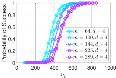
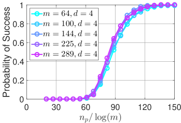

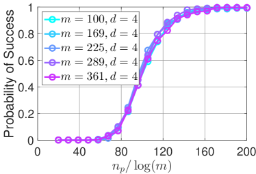
6.1 versus
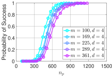
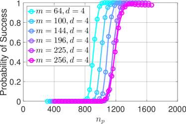
We now illustrate above effects via experiments. Since the density ratio estimator involves two sets of data with size and , to avoid complication, we first set to a sufficiently large value (), and examine the relationship between and with fixed. The results in Figure 1 show, all success rate curves align well over MNs of different sizes for both “lattice” or randomly shaped structures.
6.2 Changing
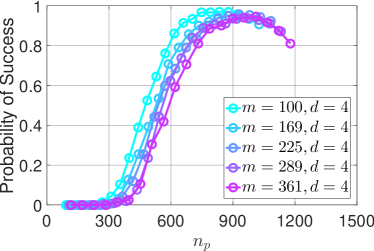
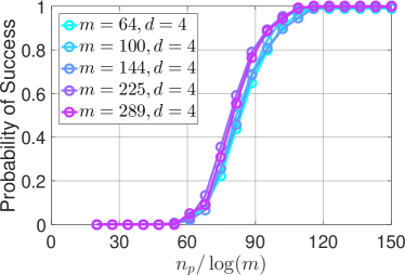
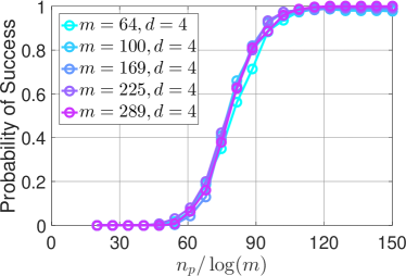
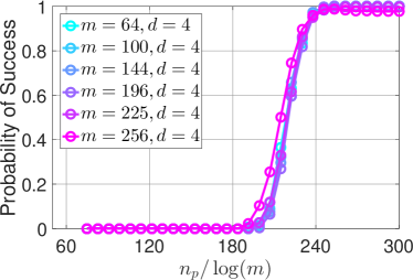
Our theorem also states that should also satisfy a certain relationship with . In this experiment, we vary to observe the change of success rate pattern using the “random” and “lattice” dataset in the previous experiment. As we can see from Figure 2(b), when , we cannot reach 100% success rate even for an ever growing and the probability of success even decays in the final stage. This can be explained by (13) in Theorem 1. If is large enough, the second term in (13) can be safely ignored. However, as decays when grows, a small may not be able to suppress the second term and the overall probability of success starts to decay eventually. By setting we obtain a perfectly aligned result (Figure 2(c)), as our theorem indicated. It also shows that though is required to grow quadratically with , it can be rescaled by a small constant (in this case, 0.01). Moreover, Corollary 3 points out if the density ratio model is bounded, we may relax the coupling condition between and . To verify this, we truncate a Gaussian distribution by rejecting samples fall out of a ball centered at origin with radius 15, then let . From Figure 2(d) we can see a similar patter of success rates alignment.
6.3 Changing
As Theorem 1 indicates, should grow at least quadratically with , the number of changed edges. However, in our experiments, it shows such condition is overly conservative. Figure 3(a) shows the success rate depends on only very mildly (see needed for success rates passing 80%), which is a good news. This indicates that the bound can be tightened under certain regimes.
6.4 Non-Gaussian distribution
We next perform experiments on the truncated “8”-shaped distribution (see Figure 9 in Appendix for details). The MNs are constructed as lattices, and the samples are generated via slice sampling [16]. Figure 3(c) shows, for the lattice grids with dimensions , the curves of success rates are well-aligned with the setting .
6.5 Comparison with Differential Network Leanring
In this section, we conduct experimental comparison between KLIEP and the differential network learning proposed in [33]. where the following constrained objective is minimized:
where and are the sample covariance matrices, is a small constant and is the estimated differential network. To obtain a sparse solution, Zhao et al. thresholds the solution at a certain level , i.e. for all that is thresholded to .
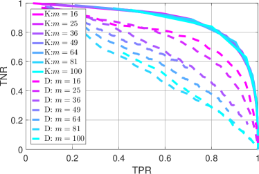
We compare the performance between KLIEP and differential network learning by Receiver Operating Characteristic (ROC) plot of True Positive and True Negative rate described in [33]. See Appendix E for more detailed settings. Experimental data are constructed using the synthetic Gaussian 4-neighbor lattice MN grid described in Section 6.1. However, instead of fixing some key variables, we adopt a more practical setting: and (i.e. the number of changed edges increases with ). The ROC curves of KLIEP (solid) and the differential method (dashed) are reported in Figure 3(d).
As it can be seen from Figure 3(d), KLIEP performs consistently better than the differential network learning method. Particularly, when and increases, the performance almost remains the same for KLIEP while for the differential method, it decays significantly.
Figure 3(d) is plotted up to , due to the fact that the differential method fails to return an output within a reasonable amount of time ( hours) when is scaled up to , using either authors’ or our implementation. This is consistent with the authors’ claim in [33], where the differential method requires more than hours to obtain the result for a MN sized . As for KLIEP, we can compute a full ROC curve within hours even for when .
7 Gene Expression Analysis
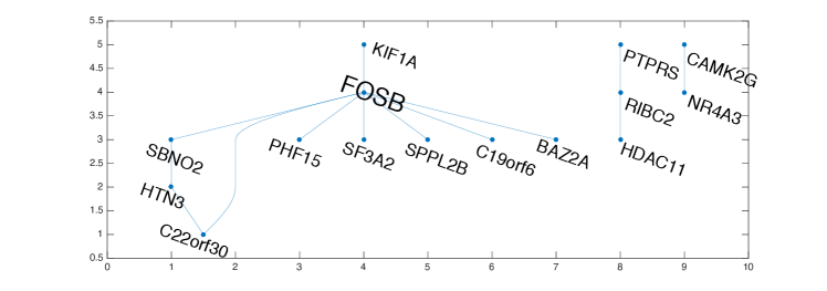
We applied KLIEP to gene expression profiles for estimating changes in gene networks activated by two different stimuli: epidermal growth factor (EGF) and heregulin (HRG). EGF is known to induce proliferation in MCF7 human breast cancer cells, while HRG induces differentiation. We used the gene expression data from [15]. The expression profiles were from cells stimulated with two controls, resulting in 29 EGF and 28 HRG sample conditions (). We extracted 1,835 genes () from the gene set in [15] by selecting genes with high expression variance (at least three times the mean of all variances). The values were log2-transformed and normalized using the 2% trimmed mean before finally getting the respective ratios with the controls. The change graph is obtained by reducing the regularization parameter until .
Figure 4 shows a learned change network. Each node represents a gene, and each edge indicates that the regulation between them is different from EGF stimuli to HRG stimuli. The leftmost large component includes 10 genes and 10 interactions, and a hub node of the component is the FOSB gene, which is a member of the Fos family of transcription factors, regulating expressions of other genes. This indicates that KLIEP successfully found that FOSB regulates other genes without any prior knowledge, and suggests that the regulation has been changed between stimuli. Moreover, FOSB is known as a regulator of cell proliferation and differentiation [15], showing that the detected change network agrees with biological knowledge. The result confirms that KLIEP can detect known biologically significant changes from the expression data. We also swapped and , and confirmed that detected changes are similar.
To evaluate the reliability of this experiment, we also conducted bootstrap experiments which are detailed in Section F in the Appendix.
8 Discussion
Let’s further discuss some properties of KLIEP.
8.1 Asymmetry of KLIEP
It can be noticed that KLIEP is asymmetric, i.e. the structural change learning performance may differ when swapping and . This is caused by directly parametrizing the density ratio which is naturally asymmetric. Such asymmetry is also reflected in Theorem 1, where the sample complexity is not the same as and , though they are “symmetrized” in Corollary 3 as under the stronger bounded ratio assumption (Assumption 7). These analysis shed some light on choosing and in practice when two datasets are given: should be “wide” and more “spread-out” compared to , so that the boundedness of the density ratio can be guaranteed, since a “sharp” would lead to very sharp and unbounded density ratio. This insight implies that KLIEP is in fact a directional method, and achieves better performance when the change itself shows a tendency of evolving from one “general” state to another more “specialized” state.
Symmetric measures of differences between densities are also available without using the density ratio, such as -2 distance [23]. In general, such difference cannot be parameterized using the difference between parameters of individual MNs, thus cannot serve as a difference measure for direct structure change learning. An alternative is the differential network learning [33] where the objective function is symmetric for both and . However such an objective is only sensible when both and are Gaussian and it cannot be easily generalized to non-Gaussian cases.
Moreover, inspired by Corollary 3, we may consider a “symmetrized” version of KLIEP by learning and independently, after which we mark changing edges by taking the union of two sparsity patterns in both models. For the support recovery probability, we simply need a union bound applied on the current results. Such a union-support algorithm is similar to the node-wise regression that is discussed in [18].
8.2 Comparison with Differential Network Learning [33]
Other than the asymmetry issues mentioned above, the theoretical analysis in this work and the one in [33] share some key similarities and both have good guarantees in high dimensional setting. First, they both set assumptions on the true difference/changes between two MNs. In [33], such a constrain is explicitly expressed: The true differential network is bounded by a constant that does not grow with (Condition 1, [33]). In our analysis, the assumption is implicitly made via limiting the “smoothness” of the density ratio (Assumptions 5, 6, 7, 9). Second, differential network learning prohibits strong “connections” among covariates. It assumes the magnitude of off-diagonal values in the covariance matrices decays as the number of changed edges increases (Condition 2, [33]), while in our work, we assume feature vectors on unchanged edges should not have strong correlations with those on changed edges (Assumption 2). Both assumptions are imposed to satisfy the incoherence condition [5] needed for Lasso-type model selection. The convergence results are also similar: The required sample size scales with for differential network learning (Theorem 2, [33]) and KLIEP (); The difference between the true parameter and the estimated one vanishes at the speed of in the -2 norm. However, we manage to achieve this rate without any assumptions of Gaussianity, while differential network learning described in [33] cannot be directly applied on non-Gaussian MNs.
8.3 Joint Structural Change Learning
Another emerging trend in graphical model structural learning is to learn multiple similar MNs simultaneously [3]. For example, one may use the following fused-lasso penalized objective function to learn -Gaussian MNs at the same time:
| (22) |
where is the negative Gaussian MN log-likelihood parametrized by precision matrix and the assumption is that all share a similar structure. Though the final outputs are estimated sparse precision matrices, one may still obtain a differential graph by taking the differences. We refer the readers to [12] for more empirical comparisons between KLIEP and Fused-lasso differential network learning.
Following the same spirit, the KLIEP based change detection can also be utilized to learn changes from -MNs at the same time by assuming all MNs sharing a similar structure, and one of the options is
| (23) |
where is the KLIEP log-likelihood of density ratio , are the triples from and by definition we have
and let .
The objective described in (22) still requires a tractable likelihood and cannot be easily generalized to non-Gaussian models. It also assumes each individual MN is sparse. However, the variation of KLIEP given in (23) does not impose any assumptions on each individual MNs and can be computed even in non-Gaussian cases. We will explore this algorithm and other possible alternatives in future works.
8.4 Uncertainty of Estimation
In this work, we have only focused on the successful change detection (Theorem 1) which states converges to one eventually. However, under very a low sample regime, the learned change structure may have high uncertainty, i.e., the results may be sensitive to some minor modifications or the randomness of the dataset. This would degrade the reliability of the obtained results. To evaluate such an uncertainty, we performed bootstrap experiments on the gene dataset used in Section 7, and the results are presented in Section F in the Appendix. Such a method is useful for practitioners to measure the reliability of an estimated network. However, the rigours quantification of such an uncertainty is still an open question and would be an important future direction to pursue.
References
- Banerjee et al. [2008] O. Banerjee, L. El Ghaoui, and A. d’Aspremont. Model selection through sparse maximum likelihood estimation for multivariate Gaussian or binary data. Journal of Machine Learning Research, 9:485–516, March 2008.
- Boyd and Vandenberghe [2004] S. Boyd and L. Vandenberghe. Convex Optimization. Cambridge University Press, Cambridge, UK, 2004.
- Danaher et al. [2014] P. Danaher, P. Wang, and D. M. Witten. The joint graphical lasso for inverse covariance estimation across multiple classes. Journal of the Royal Statistical Society: Series B (Statistical Methodology), 2014.
- Das and Bapat [2005] K.C. Das and R.B. Bapat. A sharp upper bound on the largest laplacian eigenvalue of weighted graphs. Linear Algebra and its Applications, 409(0):153 – 165, 2005. Special Issue in honor of Pauline van den Driessche.
- Donoho and Huo [2001] D. L. Donoho and X. Huo. Uncertainty principles and ideal atomic decomposition. IEEE Transactions on Information Theory, 47(7):2845–2862, 2001.
- Friedman et al. [2008] J. Friedman, T. Hastie, and R. Tibshirani. Sparse inverse covariance estimation with the graphical lasso. Biostatistics, 9(3):432–441, 2008.
- Hammersley and Clifford [1971] J. M. Hammersley and P. Clifford. Markov fields on finite graphs and lattices. 1971.
- Horn and Johnson [1986] R. A. Horn and C. R. Johnson, editors. Matrix Analysis. Cambridge University Press, New York, NY, USA, 1986.
- Kolar and Xing [2012] M. Kolar and E. P. Xing. Estimating networks with jumps. Electronic Journal of Statistics, 6:2069–2106, 2012.
- Koller and Friedman [2009] D. Koller and N. Friedman. Probabilistic Graphical Models: Principles and Techniques. MIT Press, Cambridge, MA, USA, 2009.
- Lee et al. [2007] S.-I. Lee, V. Ganapathi, and D. Koller. Efficient structure learning of Markov networks using -regularization. In B. Schölkopf, J. Platt, and T. Hoffman, editors, Advances in Neural Information Processing Systems 19, pages 817–824, Cambridge, MA, USA, 2007. MIT Press.
- Liu et al. [2014] S. Liu, J. A. Quinn, M. U. Gutmann, T. Suzuki, and M. Sugiyama. Direct learning of sparse changes in markov networks by density ratio estimation. Neural Computation, 26(6):1169–1197, 2014.
- Meinshausen and Bühlmann [2006] N. Meinshausen and P. Bühlmann. High-dimensional graphs and variable selection with the lasso. The Annals of Statistics, 34(3):1436–1462, 06 2006.
- Merris [1994] R. Merris. Laplacian matrices of graphs: a survey. Linear algebra and its applications, 197:143–176, 1994.
- Nagashima et al. [2007] T. Nagashima, H. Shimodaira, K. Ide, T. Nakakuki, Y. Tani, K. Takahashi, N. Yumoto, and M. Hatakeyama. Quantitative transcriptional control of erbb receptor signaling undergoes graded to biphasic response for cell differentiation. Journal of biological chemistry, 282(6):4045–4056, 2007.
- Neal [2003] R. M Neal. Slice sampling. The Annals of Statistics, 31(3):705–741, 2003.
- Raskutti et al. [2009] G. Raskutti, B. Yu, M. J. Wainwright, and P. Ravikumar. Model selection in gaussian graphical models: High-dimensional consistency of -regularized mle. In D. Koller, D. Schuurmans, Y. Bengio, and L. Bottou, editors, Advances in Neural Information Processing Systems 21, pages 1329–1336. Curran Associates, Inc., 2009.
- Ravikumar et al. [2010] P. Ravikumar, M. J. Wainwright, and J. D. Lafferty. High-dimensional Ising model selection using -regularized logistic regression. The Annals of Statistics, 38(3):1287–1319, 2010.
- Robert and Casella [2005] C. P. Robert and G. Casella. Monte Carlo Statistical Methods. Springer-Verlag, Secaucus, NJ, USA, 2005.
- Steinwart and Christmann [2008] I. Steinwart and A. Christmann. Support vector machines. Springer Science & Business Media, 2008.
- Sugiyama et al. [2008] M. Sugiyama, S. Nakajima, H. Kashima, P. von Bünau, and M. Kawanabe. Direct importance estimation with model selection and its application to covariate shift adaptation. In J. C. Platt, D. Koller, Y. Singer, and S. T. Roweis, editors, Advances in Neural Information Processing Systems 20. Curran Associates, Inc., 2008.
- Sugiyama et al. [2012] M. Sugiyama, T. Suzuki, and T. Kanamori. Density Ratio Estimation in Machine Learning. Cambridge University Press, Cambridge, UK, 2012.
- Sugiyama et al. [2013] M. Sugiyama, T. Kanamori, T. Suzuki, M.C. Plessis, S. Liu, and I. Takeuchi. Density-difference estimation. Neural Computation, 25(10):2734–2775, 2013.
- Tibshirani et al. [2005] R. Tibshirani, M. Saunders, S. Rosset, J. Zhu, and K. Knight. Sparsity and smoothness via the fused lasso. Journal of the Royal Statistical Society: Series B (Statistical Methodology), 67(1):91–108, 2005.
- Tomioka and Suzuki [2014] R. Tomioka and T. Suzuki. Spectral norm of random tensors. arXiv preprint arXiv:1407.1870, 2014.
- Tsuboi et al. [2009] Y. Tsuboi, H. Kashima, S. Hido, S. Bickel, and M. Sugiyama. Direct density ratio estimation for large-scale covariate shift adaptation. Journal of Information Processing, 17:138–155, 2009.
- Wainwright [2009] M. J. Wainwright. Sharp thresholds for high-dimensional and noisy sparsity recovery using l1-constrained quadratic programming (lasso). IEEE Trans. Inf. Theor., 55(5):2183–2202, May 2009.
- Wasserman [2010] L. Wasserman. All of Statistics: A Concise Course in Statistical Inference. Springer Publishing Company, Incorporated, 2010.
- Yamada et al. [2013] M. Yamada, T. Suzuki, T. Kanamori, H. Hachiya, and M. Sugiyama. Relative density-ratio estimation for robust distribution comparison. Neural Computation, 25(5):1324–1370, 2013.
- Yang et al. [2012] E. Yang, A. Genevera, Z. Liu, and P. Ravikumar. Graphical models via generalized linear models. In F. Pereira, C.J.C. Burges, L. Bottou, and K.Q. Weinberger, editors, Advances in Neural Information Processing Systems 25, pages 1358–1366. Curran Associates, Inc., 2012.
- Yuan and Lin [2006] M. Yuan and Y. Lin. Model selection and estimation in regression with grouped variables. Journal of the Royal Statistical Society: Series B (Statistical Methodology), 68(1):49–67, 2006.
- Zhang and Wang [2010] B. Zhang and Y.J. Wang. Learning structural changes of Gaussian graphical models in controlled experiments. In Proceedings of the Twenty-Sixth Conference on Uncertainty in Artificial Intelligence (UAI2010), pages 701–708, 2010.
- Zhao et al. [2014] S. Zhao, T. Cai, and H. Li. Direct estimation of differential networks. Biometrika, 101(2):253–268, 2014.
-
Appendix A Image Change Detection

(a) 4:30PM, 7th Mar, 2016 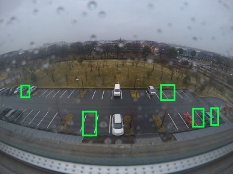
(b) 5:30PM, 7th Mar, 2016 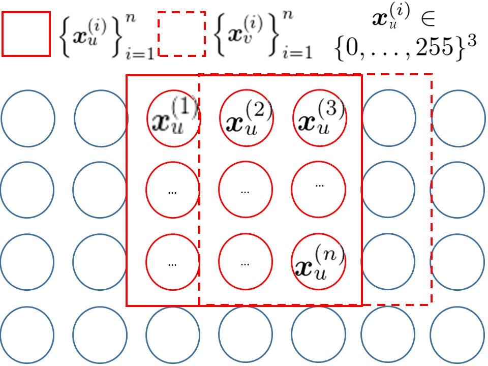
(c) Construct samples using sliding windows (red boxes). 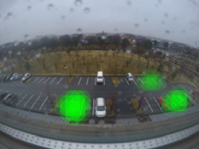
(d) Detected changes, we set Figure 5: Detecting changes of parking patterns from two photos. Two photos were taken in a rainy afternoon using a camera pointing at the parking lot of ISM. In this task, we are interested in learning the changes of the parking patterns marked by green boxes in Figure 5(b). As we can see from Figure 5(a) and 5(b), the light conditions and positions of raindrops vary in two pictures.
To construct samples, we use windows of pixels (Figure 5(c)). Each window is a dimension of a dataset, and the samples are the pixel RGB values within this window. By sliding the window across the entire picture, we may obtain samples of different dimensions. Two sets of data can be obtained by using this sample generating mechanism over two images.
Assuming an image can be represented by an MN of windows, changes of pixels values within a window may cause changes of “interactions” between neighboring windows. In other words, we can discover a change by looking at the change of the dependency of pixel values between a certain window and its neighbours. This is more advantageous than simply looking at the pixel values since changing the brightness of a picture may increase the pixel values in many windows simultaneously, even if the “contrast” between two windows does not change by much.
By applying KLIEP on such two sets of data and highlighting adjacent window pairs that are involved in the changes of pairwise interactions, we may spot changes between two images. In our experiment, we use sliding windows of size on a image, generating two sets of samples with and . We reduce until . The spotted changes were plotted in Figure 5(d). It is can be seen that KLIEP has correctly labeled almost all changed parkings between two images except one missing on the left.
Appendix B Proofs
B.1 Proof of Lemma 1
In the appendix, we denote as the negative likelihood objective function .
Proof.
Consider two optimals of (9), has the correct sparsity over zero elements. We have the following equality
(24) noting ,
(25) substituting (25) into (24) we have the following inequality:
Due to convexity of and as stated in (14), the leftmost term is further lower bounded as:
The above suggests all the inequality we have used to lower-bound should take the exact equality. Therefore (25) should take the exact equality:
which holds only if , given .
Moreover, if is invertible, it can be shown that is the unique solution. ∎
B.2 Proof of Lemma 2
Before proving the lemma, we show the boundedness of the deviation between true normalization term and sample approximated term . For conveniences, we denote as and as .
Proposition 12.
For any vector such that and some constant ,
(26) Proof.
Similarly,
Applying union bound, we can get
Set , then
particularly when , which is often the case in practice,
(27) by using the fact that when (see Figure. 6).
Figure 6: The plot of 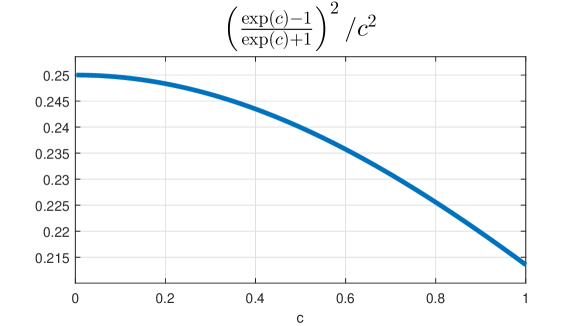
∎
We then introduce the proof of Lemma 2:
Proof.
To bound where , we may show is bounded.
The direct boundedness of could be difficult to prove, however we can investigate the bound of the inner product where is a zero padding sign vector with only non-zero elements on sub-vector indexed by . Since ,
bound each summand indexed by is sufficient.
In order to use Chernoff bounding technique, we look into the moment generating function of . Since after a few lines of algebra we have
where and . Take logarithm on both sides,
Now, define the event,
(28) Note that given Then the following holds conditioned on event :
(29) Then applying Taylor expansion to (29),
(30) where the is a vector between and in coordinate fashion.
Finally, applying the Chernoff bounding technique:
and
Finally, exponentiate both sides and set , we have
Since there exists a sign vector so that , therefore, we can conclude:
Consider a vector with sub-vectors, we can bound by union bound:
When and ,
Let , then for
we can have in high probability.
Moreover, by using the fact that
we can obtain
for constants and . By substituting and replace with its lower bound, we complete the proof. ∎
B.3 Proof of Lemma 3
Proof.
Since we are trying to prove that , where , according to [18, 30], we may construct the following function:
(31) where is a convex function, , reaches the minimal at and . Simple proof in [18] can show that for a if , .
We first use Taylor expansion on the first two terms of (31),
(32) Since for the first and the last term
(33) and
(34) we only need to lower-bound the middle term.
B.4 Proof of Lemma 4
Since
by applying the Mean-value theorem, we get
B.5 Proof of Lemma 5
Proof.
We know that
so now we show by using the boundedness of implied from Assumption 7, this converges to in probability.
First we show that can be upper-bounded by:
We now need Hoeffding inequality for norm-bounded vector random variables which has appeared in previous literatures such as [20]: For a set of bounded zero-mean vector-valued random variable , we have
for all Now it is easy to see
(39) as long as
(40) As to , it can be upper-bounded by
and using regular Hoeffding-inequality we may obtain:
(41) Therefore, combining (39) and (41):
where is a constant defined as . Applying the union-bound for all ,
and when ,
where is a constant. Assume that and we set as
thus (40), the condition of using vector Hoeffding-inequality is satisfied. ∎
B.6 Proof of Corollaries
Proof of Corollary 1
Consider an event which is slightly different from (28):
Note that under the new Assumption 6, we will have
given . Note here the extra is needed on the denominator of RHS. The derivation is the same as what has been used in Proposition 12.
Then the following holds conditioned on :
Since
by following the similar techniques in Lemma 2, it can be shown that
Using the same derivation in Lemma 2, we will reach the conclusion that for
we can have with high probability.
Again, by using the fact that
we can obtain
for constants and . By substituting and replace with its lower bound, we get:
Proof of Corollary 2
For basis function where at most fixed-location elements are non-zero (irrelevant to ),
may have at most non-zero elements. Therefore, consider a sign vector with non-zero elements is sufficient, i.e. . Instead of (B.2), we have the following inequality:
Follow the derivation of Lemma 2, we may get the boundedness of as stated in Corollary 2.
Furthermore, for a sign vector only allowed to take values on a length sub-vector, where only elements can be non-zero, the number of possibilities is , and after applying the union bound
we can obtain
B.7 Proof of Proposition 5
Proof.
Let’s define the -input log-sum-exp function as , then the sample Fisher information matrix, can be written as
Using the chain-rule and matrix notation, we may write the second-order derivative as
where is a matrix that each column , and . Therefore,
(42) The second-order derivative of log-sum-exp function can be found in previous literatures [2], and is a positive semi-definite matrix.
where is a column vector, and the operator “” of a vector with length is to set the elements of as the diagonal of a diagnoal-matrix.
It can be observed that the elements in are all strictly negative except the diagonal elements, which are the negative sums of the elements in the same column. is a Laplacian matrix [14] of a fully connected graph, with strictly positive weights. The upper-bound of maximum eigenvalue of a Laplacian matrix has been studied in great detail, such as Corollary 3.2, [4]. Restate using our notation:
(43) The last line is due to Assumption 7 given , and . It can be seen immediately that as long as is bounded, then is bounded. ∎
B.8 Proof of Proposition 6
Proof.
To simplify the notation, we actually prove the boundedness of . Using the exact same set of assumptions, we can prove is bounded using the same strategy.
It can be shown that .
From multiplicative rule, we have
where and is still a Laplacian matrix whose -th elements can be written as
Similarly to the bounding techniques used in (B.7), we have
(44) given , and . As a result,
(45) By the construction of , we can see that,
Therefore,
(46) by using the fact that .
B.9 Proof of Proposition 7
Proof.
Recall
Since the Laplacian matrix in the middle always has the smallest eigenvalue 0, while is always positive semi-definite, we are guaranteed to have a trivial lower bound of the smallest eigenvalue 0 without utilizing any assumptions. However, by the construction of the Laplacian we can see
Therefore
Note that is always positive semi-definite. By Assumption 7, , if , . Therefore
∎
B.10 Proof of Proposition 8
Proof.
∎
B.11 Proof of Proposition 9
Proof.
Since
we just need to show
holds with high probability. So we bound the tail probability of this event
The rest is simply based on the concentration property of the sums of bounded zero-mean random variable . Now we can conclude
then we have holds with high probability. ∎
B.12 Proof of Proposition 10
Proof.
The boundedness of zero-mean random variable guarantees its exponentially decaying tail behavior via standard Hoeffding inequality, i.e.,
∎
B.13 Proof of Proposition 11
Proof.
Since , we conclude the proof. ∎
Appendix C The Derivatives of Negative KLIEP Log-likelihood
Proposition 13.
The second-order derivative is the importance sampled covariance using samples from . Moreover, the third-order derivative is the importance-sampled skewness using samples from :
where is a scalar.
Appendix D Experimental Settings of Success Rate Plots
Define two edge sets for MN and as and separately. In experiments with Gaussian distributions, densities are constructed as
where , . are set to be the same as while for randomly picked edges, .
As to the “8-shaped” distribution, its pairwise potentials are introduced in Figure 9. We set . is constructed from with randomly removed edges.
Appendix E Experimental Settings of Comparison with Differential Network Leanring
We adopt the True Positive (TP) and True Negative (TN) rate as described in [33]:
where is the indicator function. For KLIEP, we compute a sequence of TPR and TNR from by changing the regularization parameter . For differential network learning, we obtain for different choices of , and compute TPR and TNR by varying the threshold for each . All TPR and TNR values are averaged over at least 25 random trials. Then the curve corresponds to that maximizes the Area Under the Curve (AUC) is plotted.
Appendix F Bootstrap of Gene Expression Dataset
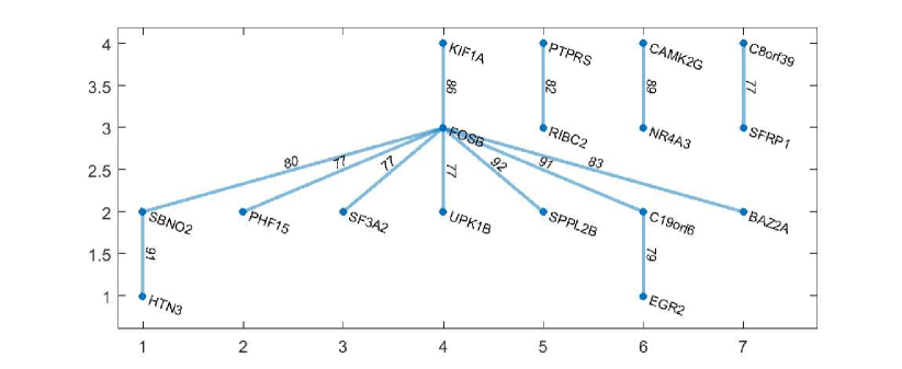
Figure 7: Edges appear more than 75 times out of 100 bootstrap trials. To assess the reliability of the results obtained in Section 7, we have also conducted bootstrap random trials on this dataset. Datasets are re-sampled from both and and the experiments are repeated for 100 times. After counting the edges appearing in the estimated graph structures we plot the graph in Figure 7 whose edges appear at least 75 times out of our 100 trails. Nodes are names of genes, and the labels on the edges are the numbers of occurrences.
It can be seen that the obtained differential network is very close to the one we presented in Figure 4, and the main structure (“the hub” around the FOSB gene) remains a dominant feature in the graph, thus this does not change our conclusion that the FOSB is a regulator of other genes.
(a) One-dimensional Gaussian distributions and their density ratios. Assumptions 7 and 9 can be applied to the 0-bounded density ratio (green line). Our Assumptions 5 and 6 can partially cover the totally unbounded density ratio model with some exceptions (such as the green dashed Gaussian density ratio, which grows too violently). Figure 8: The comparison between different boundedness assumption 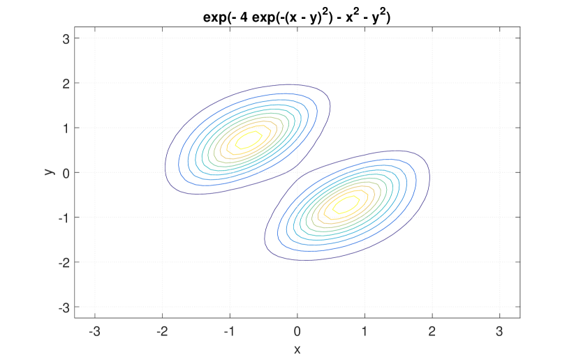
Figure 9: Contour plot for 2D “8-shaped Distribution” with correlation between dimension and . The distribution is truncated over a ball centered at origin with radius of 15. 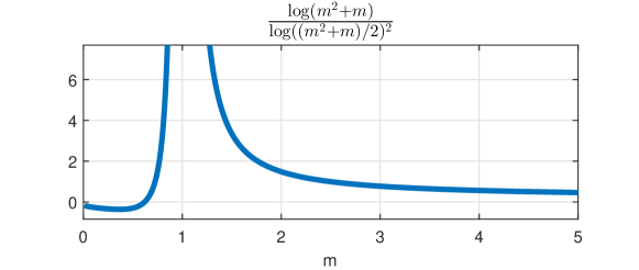
Figure 10: The plot of . Appendix G Illustrations
G.1 Applicability of Smoothness Assumptions
Figure 8 illustrates the applicability of our assumptions using one-dimensional Gaussian distributions.
G.2 Contours of non-Gaussian Distributions
G.3 Plot of
