Classification-based Approximate Policy Iteration: Experiments and Extended Discussions

Abstract

Tackling large approximate dynamic programming or reinforcement learning problems requires methods that can exploit regularities, or intrinsic structure, of the problem in hand. Most current methods are geared towards exploiting the regularities of either the value function or the policy. We introduce a general classification-based approximate policy iteration (CAPI) framework, which encompasses a large class of algorithms that can exploit regularities of both the value function and the policy space, depending on what is advantageous. This framework has two main components: a generic value function estimator and a classifier that learns a policy based on the estimated value function. We establish theoretical guarantees for the sample complexity of CAPI-style algorithms, which allow the policy evaluation step to be performed by a wide variety of algorithms (including temporal-difference-style methods), and can handle nonparametric representations of policies. Our bounds on the estimation error of the performance loss are tighter than existing results. We also illustrate this approach empirically on several problems, including a large HIV control task.

I Introduction

We consider the problem of finding a near-optimal policy (i.e., controller) for discounted Markov Decision Processes (MDP) with large state space and finite action space [11, 58, 59]. We focus on the scenario where the MDP model is not known and we only have access to a batch of interaction data. For problems with large state spaces (e.g., when the state space is $\mathbb{R}^{d}$ with large $d$), finding a close-to-optimal policy is difficult (due to the so-called curse of dimensionality) unless one benefits from regularities, or special structure, of the problem in hand, e.g., smoothness or sparsity of the value function or the optimal policy. Many successful algorithms developed in reinforcement learning (RL) and approximate dynamic programming (ADP) focus on exploiting regularities of the value function, e.g., Farahmand et al. [27, 26], Kolter and Ng [41], Taylor and Parr [60], Ghavamzadeh et al. [37], Farahmand and Precup [24]. However, useful structure can also arise in the policy space. For instance, in many control problems, simple policies such as bang-bang or PID controllers can perform quite well if tuned properly. Direct policy search algorithms and various policy gradient algorithms try to exploit such structure, e.g., Baxter and Bartlett [9], Marbach and Tsitsiklis [48], Kakade [39], Cao [16], Ghavamzadeh and Engel [35].

The aforementioned methods exploit only one type of regularity (either value or policy), therefore they do not benefit from all potential regularities of a problem. The goal of this paper is to introduce a class of algorithms, which we call Classification-based Approximate Policy Iteration (CAPI), that can potentially benefit from the regularities of both value function and policy.

The inspiration for our approach comes from existing classification-based RL algorithms, e.g., Lagoudakis and Parr [44], Fern et al. [32], Li et al. [47], Lazaric et al. [45]. These methods use Monte Carlo trajectories to roughly estimate the action-value function of the current policy (i.e., the value of choosing a particular action at the current state and then following the policy) at several states. This approach is called a rollout-based estimate by Tesauro and Galperin [61] and is closely related, but not equivalent, to the rollout algorithms of Bertsekas [10]. In these methods, the rollout estimates at several points in the state space define a set of (noisy) greedy actions (positive examples) as well as non-greedy actions (negative examples), which are then fed to a classifier. The classifier “generalizes” the greedy action choices over the entire state space. The procedure is repeated.

Classification-based methods can be interpreted as variants of Approximate Policy Iteration (API) that use rollouts to estimate the action-value function (policy evaluation step) and then project the greedy policy obtained at those points onto the predefined space of controllers (policy improvement step).

In many problems, this approach is helpful for three main reasons. First, good policies are sometimes simpler to represent and learn than good value functions. Second, even a rough estimate of the value function is often sufficient to separate the best action from the rest, especially when the gap between the value of the greedy actions and the rest is large. And finally, even if the best action estimates are noisy (due to value function imprecision), one can take advantage of powerful classification methods to smooth out the noise.

Rollout-based estimator of the value function, however, does not generalize the value function over the state space, and instead produces estimates at a finite collection of points. This lack of generalization makes rollout-based estimators data-inefficient. This is a big concern in real problems, in which new samples may be expensive or impossible to generate, e.g., adaptive treatment strategies or user dialogue systems. Moreover, one cannot easily use rollouts when only access to a batch of data is allowed and a generative model or simulator of the environment is not available.

To address the limitation of rollout-based estimators, we propose the CAPI framework. CAPI generalizes the current classification-based algorithms by allowing the use any policy evaluation method including, but not limited to, rollout-based estimators (as in previous work [44, 45]), LSTD [43, 46], modified Bellman Residual Minimization [3], the policy evaluation version of Fitted Q-Iteration [21, 52, 15, 24], and their regularized variants [27, 37, 26], as well as online methods for policy evaluation such as Temporal Difference learning [58, 62] and GTD [57]. This is a significant generalization of existing classification-based RL algorithms, which become special cases of CAPI. Our theoretical results indicate that this extension is indeed sound.

On a more technical note, the loss function used for the classification step of CAPI is different from the conventional $0/1$-loss of classification, and is weighted according to the difference between the value of the greedy actions and the selected action. The $0/1$-loss penalizes all mistakes equally and does not consider the relative importance of different regions of the state space, which may lead to surprisingly bad policies (cf. Section V). In contrast, the use of weighted loss ensures that the resulting policy closely follows the greedy policy in regions of the state space where the difference between the best action and the rest is considerable (so choosing the wrong action is costly), but pays less attention to regions where all actions are almost the same. The choice of weighted loss in RL/ADP is not entirely new and has been used in the context of classification-based RL (Li et al. [47], Lazaric et al. [45], Gabillon et al. [33], Scherrer et al. [55]) and elsewhere (Conservative Policy Iteration approach of Kakade and Langford [40] and a variant of Policy Search by Dynamic Programming of Bagnell et al. [5]).

The main theoretical contribution of this paper is the finite-sample error analysis of CAPI-style algorithms, which allows general policy evaluation algorithms, handles nonparametric policy spaces, and provides a faster convergence rate for the estimation error than existing results. Using nonparametric policies is a significant extension of the work by Fern et al. [32], which is limited to finite policy spaces, and of Lazaric et al. [45] and Gabillon et al. [33], which are limited to policy spaces with finite Vapnik-Chervonenkis (VC) dimension. Our faster convergence rates are due to using a concentration inequality based on the powerful notion of local Rademacher complexity [7], which is known to lead to fast rates in supervised learning.

We also leverage the notion of action-gap regularity, recently introduced by Farahmand [23], which implies that choosing the right action at each state may not require a precise estimate of the action-value function. When the action-gap regularity of the problem is favourable, the convergence rate of CAPI is faster than the convergence rate of the estimate of the action-value function (and without any assumption on that regularity, the convergence rate is the same).

Another theoretical contribution of this work is a new error propagation result that shows that the errors at later iterations of CAPI play a more important role on the performance of the resulting policy. So, if one has finite resources (samples or computational time), it is better to spend effort on the estimation at later iterations (by using a better function approximator, more samples, etc).

We illustrate CAPI’s flexibility on some standard toy problems, as well as on a large HIV control domain, which is known to be difficult.

II Background and Notation

In this section, we summarize necessary definitions and notation. For more information, we refer the reader to Bertsekas and Tsitsiklis [11], Sutton and Barto [58], Szepesvári [59].

II-A Markov Decision Processes

For a space $\Omega$ with $\sigma$-algebra $\sigma_{\Omega}$, $\mathcal{M}(\Omega)$ denotes the set of all probability measures over $\sigma_{\Omega}$. The space of bounded measurable functions with respect to (w.r.t.) $\sigma_{\Omega}$ is denoted by $B(\Omega)$ and $B(\Omega,L)$ denotes the subset of $B(\Omega)$ with bound $0<L<\infty$.

A finite-action discounted MDP is a 5-tuple $({\mathcal{X}},{\mathcal{A}},\mathcal{P},\mathcal{R},\gamma)$, where ${\mathcal{X}}$ is a measurable state space, ${\mathcal{A}}$ is a finite set of actions, $\mathcal{P}:{\mathcal{X}}\times{\mathcal{A}}\to\mathcal{M}({\mathcal{X}})$ is the transition probability kernel, $\mathcal{R}:{\mathcal{X}}\times{\mathcal{A}}\to\mathcal{M}(\mathbb{R})$ is the reward kernel, and $\gamma\in[0,1)$ is a discount factor. Assume that the expected reward is uniformly bounded by $R_{\textrm{max}}$. A measurable mapping $\pi:{\mathcal{X}}\rightarrow{\mathcal{A}}$ is called a deterministic Markov stationary policy, or just policy for short. Following a policy $\pi$ means that at each time step, $A_{t}=\pi(X_{t})$.

A policy $\pi$ induces the transition probability kernel $\mathcal{P}^{\pi}:{\mathcal{X}}\to\mathcal{M}({\mathcal{X}})$. For a measurable subset $S\subseteq{\mathcal{X}}$, we define $(\mathcal{P}^{\pi})(S|x)\triangleq\int\mathcal{P}(\mathrm{d}y|x,\pi(x)){\mathbb{I}}_{\{y\in S\}}$, in which ${\mathbb{I}}_{\{\cdot\}}$ is the indicator function. The $m$-step transition probability kernels $(\mathcal{P}^{\pi})^{m}:{\mathcal{X}}\to\mathcal{M}({\mathcal{X}})$ for $m=2,3,\cdots$ are inductively defined as $(\mathcal{P}^{\pi})^{m}(S|x)\triangleq\int_{{\mathcal{X}}}\mathcal{P}(\mathrm{d}y|x,\pi(x))(\mathcal{P}^{\pi})^{m-1}(S|y)$.

Given a transition probability kernel $\mathcal{P}^{\prime}:{\mathcal{X}}\to\mathcal{M}({\mathcal{X}})$, the right-linear operator $\mathcal{P}^{\prime}\cdot:B({\mathcal{X}})\to B({\mathcal{X}})$ is defined as $(\mathcal{P}^{\prime}V)(x)\triangleq\int_{{\mathcal{X}}}\mathcal{P}^{\prime}(\mathrm{d}y|x)V(y)$. In other words, $(\mathcal{P}^{\prime}V)(x)$ is the expected value of $V$ w.r.t. the distribution induced by following $\mathcal{P}^{\prime}$ from state $x$. For a probability distribution $\rho\in\mathcal{M}({\mathcal{X}})$ and a measurable subset $S\subseteq{\mathcal{X}}$, let the left-linear operators $\cdot\mathcal{P}^{\prime}:\mathcal{M}({\mathcal{X}})\to\mathcal{M}({\mathcal{X}})$ be $(\rho\mathcal{P}^{\prime})(S)=\int\rho(dx)\mathcal{P}^{\prime}(\mathrm{d}y|x){\mathbb{I}}_{\{y\in S\}}$. In other words, $(\rho\mathcal{P}^{\prime})$ is the distribution induced by $\mathcal{P}^{\prime}$ when the initial distribution is $\rho$. In this paper, $\mathcal{P}^{\prime}$ is usually $(\mathcal{P}^{\pi})^{m}:\mathcal{M}({\mathcal{X}})\to\mathcal{M}({\mathcal{X}})$, for $m=1,2,\dotsc$.

The value function $V^{\pi}$ and the action-value function $Q^{\pi}$ of a policy $\pi$ are defined as follows: Let $(R_{t};t\geq 1)$ be the sequence of rewards when the Markov chain is started from state $X_{1}$ (or state-action $(X_{1},A_{1})$ for $Q^{\pi}$) drawn from a positive probability distribution over ${\mathcal{X}}$ (${\mathcal{X}}\times{\mathcal{A}}$) and the agent follows the policy $\pi$. Then $V^{\pi}(x)\triangleq{\mathbb{E}}\left[\sum_{t=1}^{\infty}\gamma^{t-1}R_{t}\,\Big{|}\,X_{1}=x\right]$ and $Q^{\pi}(x,a)\triangleq{\mathbb{E}}\left[\sum_{t=1}^{\infty}\gamma^{t-1}R_{t}\,\Big{|}\,X_{1}=x,A_{1}=a\right]$. The functions $V^{\pi}$ and $Q^{\pi}$ are uniformly bounded by $Q_{\textrm{max}}=R_{\textrm{max}}/(1-\gamma)$, independent of the choice of $\pi$.

The optimal value and optimal action-value functions are defined as $V^{*}(x)=\sup_{\pi}V^{\pi}(x)$ for all $x\in{\mathcal{X}}$ and $Q^{*}(x,a)=\sup_{\pi}Q^{\pi}(x,a)$ for all $(x,a)\in{\mathcal{X}}\times{\mathcal{A}}$. A policy ${\pi^{*}}$ is optimal if $V^{{\pi^{*}}}=V^{*}$. A policy $\pi$ is greedy w.r.t. an action-value function $Q$, denoted by $\pi=\hat{\pi}(\cdot;Q),$ if $\pi(x)=\mathop{\textrm{argmax}}_{a\in{\mathcal{A}}}Q(x,a)$ holds for all $x\in{\mathcal{X}}$ (if there exist multiple maximizers, one of them is chosen in an arbitrary deterministic manner). A greedy policy w.r.t. the optimal action-value function $Q^{*}$ is an optimal policy.

II-B Action-Gap Characterization of the MDP

The action-gap regularity [23] is a recently introduced complexity measure of a control problem, inspired by the low-noise condition in the classification literature [4]. Our theoretical analysis will rely on the notion of action-gap regularity of an MDP [23], which characterizes the complexity of a control problem. For simplicity, we define and analyze the two-action case, but the CAPI framework naturally accommodates MDPs with more actions, as we explain below.

Consider an MDP with two actions. For any $Q:{\mathcal{X}}\times{\mathcal{A}}\rightarrow\mathbb{R}$, the action-gap function is defined as

$$\mathbf{g}_{Q}(x)\triangleq|Q(x,1)-Q(x,2)|\qquad\text{for all }x\in{\mathcal{X}}.$$

To understand why the action-gap function is informative, suppose that we have an estimate $\hat{Q}^{\pi}$ of $Q^{\pi}$ and we want to perform policy improvement based on $\hat{Q}^{\pi}$. The greedy policy w.r.t. $\hat{Q}^{\pi}$, i.e., ${\hat{\pi}}(\cdot;\hat{Q}^{\pi})$, should ideally be close to the greedy policy w.r.t. $Q^{\pi}$, i.e., ${\hat{\pi}}(\cdot;Q^{\pi})$. If the action-gap $\mathbf{g}_{Q^{\pi}}(x)$ is large for some state $x$, the regret of choosing an action different from ${\hat{\pi}}(x;Q^{\pi})$, roughly speaking, is large; however, confusing the best action with the other one is also less likely. If the action-gap is small, a confusion is more likely to arise, but the regret stemming from the wrong choice will be small.

To characterize how difficult a problem is, we need to summarize the behaviour of the action-gap function over the entire state space. This is done in the following assumption.

• Assumption A1 (Action-Gap). For a fixed MDP $({\mathcal{X}},{\mathcal{A}},\mathcal{P},\mathcal{R},\gamma)$ with ${|{\mathcal{A}}|}=2$ and a fixed distribution over states $\nu\in\mathcal{M}({\mathcal{X}})$, there exist constants $c_{g}>0$ and $\zeta\geq 0$ such that for any $\pi\in\Pi$ and all $\varepsilon>0$, we have

  $${\mathbb{P}}_{\nu}\left(0<\mathbf{g}_{Q^{\pi}}(X)\leq\varepsilon\right) \triangleq\int_{{\mathcal{X}}}{\mathbb{I}}{\{0<\mathbf{g}_{Q^{\pi}}(x)\leq\varepsilon\}}\,\mathrm{d}\nu(x)\leq c_{g}\,\varepsilon^{\zeta}.$$

The value of $\zeta$ controls the distribution of the action-gap $\mathbf{g}_{Q^{\pi}}(X)$. A large value of $\zeta$ indicates that the probability of $Q^{\pi}(X,1)$ being very close to $Q^{\pi}(X,2)$ is small. This implies that the estimate $\hat{Q}^{\pi}$ can be quite inaccurate in a large subset of the state space (measured according to $\nu$), but ${\hat{\pi}}(\cdot;\hat{Q}^{\pi})$ would still be the same as ${\hat{\pi}}(\cdot;Q^{\pi})$. Note that any MDP satisfies the inequality when $\zeta=0$ and $c_{g}=1$, so the class of MDPs satisfying this property is not restricted in any way. MDPs with $\zeta=0$, however, are quite “boring” as it implies that $\mathbf{g}_{Q^{\pi}}(x)=0$ and so $Q^{\pi}(x,1)=Q^{\pi}(x,2)$ for all $x\in{\mathcal{X}}$ ($\nu$-almost surely). Trying to find policies to control these MDPs is futile after all. Also, note that one could characterize the distribution of the action-gap function in other ways too, e.g., upper bounds in a form other than $O(\varepsilon^{\zeta}$). The current form, however, simplifies the analysis while succinctly showing the effect of the action-gap distribution.

The $L_{\infty}$-norm on ${\mathcal{X}}\times{\mathcal{A}}$ is defined as $\left\|Q\right\|_{\infty}\triangleq\sup_{(x,a)\in{\mathcal{X}}\times{\mathcal{A}}}|Q(x,a)|$. We also use a definition of supremum norm that holds only on a set of points from ${\mathcal{X}}$. Let $\mathcal{D}_{n}=\{X_{1},\dotsc,X_{n}\}$ with $X_{i}\in{\mathcal{X}}$; then, $\left\|Q\right\|_{\infty,\mathcal{D}_{n}}\triangleq\max_{x\in\mathcal{D}_{n},a\in{\mathcal{A}}}|Q(x,a)|$.

III CAPI Framework

CAPI is an approximate policy iteration framework that takes a policy space $\Pi$, a distribution over states $\nu\in\mathcal{M}({\mathcal{X}})$, and the number of iterations $K$ as inputs, and returns a policy whose performance should be close to the best policy in $\Pi$. Its outline is presented in Figure 1.

Algorithm CAPI$(\Pi,\nu,K)$

  Input: Policy space $\Pi$, State distribution $\nu$, Number of iterations $K$

  Initialize: Let $\pi_{(0)}\in\Pi$ be an arbitrary policy

  for $k=0,1,\dotsc,K-1$ do

     Construct a dataset ${\mathcal{D}}_{n}^{(k)}=\{X_{i}\}_{i=1}^{n},\;X_{i}\stackrel{{\scriptstyle\text{i.i.d.}}}{{\sim}}\nu$

     $\hat{Q}^{\pi_{k}}\leftarrow\text{PolicyEval}(\pi_{k})$

     $\pi_{k+1}\leftarrow\mathop{\textrm{argmin}}_{\pi\in\Pi}\hat{L}^{\pi_{k}}_{n}(\pi)$ (action-gap-weighted classification)

  end for

Figure 1: CAPI pseudocode

PolicyEval can be any algorithm that computes an estimate $\hat{Q}^{\pi}$ of $Q^{\pi}$, including: rollout-based estimation [44, 45], LSTD-Q [43, 27], modified Bellman Residual Minimization [3], and Fitted Q-Iteration [21, 52, 26], or a combination of rollouts and function approximation [33], as well as online algorithms such as TD [62] and GTD [57].

Exploiting the intuition given by the action-gap phenomenon [23], which entails that when $\mathbf{g}_{Q^{\pi}}(x)$ is large at some state $x$, the regret of choosing an action different from ${\hat{\pi}}(x;Q^{\pi})$ is also large, the approximate policy improvement step of CAPI at each iteration $k$ is performed by minimizing the following action-gap-weighted empirical loss function in policy space $\Pi$:

$$\hat{L}^{\pi_{k}}_{n}(\pi) \triangleq\int_{{\mathcal{X}}}\mathbf{g}_{\hat{Q}^{\pi_{k}}}(x){\mathbb{I}}{\{\pi(x)\neq\mathop{\textrm{argmax}}_{a\in{\mathcal{A}}}\hat{Q}^{\pi_{k}}(x,a)\}}\,\mathrm{d}\nu_{n}$$ (1)

$$=\sum_{X_{i}\in\mathcal{D}_{n}^{(k)}}\mathbf{g}_{\hat{Q}^{\pi_{k}}}(X_{i}){\mathbb{I}}{\{\pi(X_{i})\neq\mathop{\textrm{argmax}}_{a\in{\mathcal{A}}}\hat{Q}^{\pi_{k}}(X_{i},a)\}},$$

where $\nu_{n}$ is the empirical distribution induced by the samples in $\mathcal{D}_{n}^{(k)}=\{X_{i}\}_{i=1}^{n}$ with $X_{i}\sim\nu$, i.e., $\nu_{n}=\frac{1}{n}\sum_{X_{i}\in\mathcal{D}_{n}^{(k)}}\delta_{X_{i}}$ where $\delta_{X_{i}}$ is a point mass at $X_{i}$ for $i=1,\dotsc,n$. This loss function emphasizes states in which the regret of choosing a non-greedy action is large. The policy improvement step of CAPI is defined by the following optimization problem:

$$\pi_{k+1}\leftarrow\mathop{\textrm{argmin}}_{\pi\in\Pi}\hat{L}^{\pi_{k}}_{n}(\pi)$$ (2)

Policy $\pi_{k+1}$ is the projection of the greedy policy ${\hat{\pi}}(\cdot;\hat{Q}^{\pi_{k}})$, defined only at points $\mathcal{D}_{n}^{(k)}$, onto policy space $\Pi$ when the distance measure is weighted according to the estimated action-gap function $\mathbf{g}_{\hat{Q}^{\pi_{k}}}$. This should be contrasted with the conventional classification-based approaches [44], which use a uniform weight for all states, i.e., they minimize $\int_{{\mathcal{X}}}{\mathbb{I}}{\{\pi(x)\neq\mathop{\textrm{argmax}}_{a\in{\mathcal{A}}}\hat{Q}^{\pi_{k}}(x,a)\}}\mathrm{d}\nu_{n}$. Note that the loss (1) is also used by Lazaric et al. [45], Gabillon et al. [33].

A uniformly weighted loss might lead to a bad choice of policies, as it does not take into account the relative importance of different regions in the state space. This is especially a concern if the greedy policy ${\hat{\pi}}(\cdot;\hat{Q}^{\pi_{k}})$ does not belong to $\Pi$, so that there are some points in the dataset for which ${\mathbb{I}}{\{\pi(x)\neq\mathop{\textrm{argmax}}_{a\in{\mathcal{A}}}\hat{Q}^{\pi_{k}}(x,a)\}}$ is nonzero. To simplify the discussion, suppose there are only two points $x_{1}$ and $x_{2}$. The uniformly weighted loss does not differentiate between these two points, regardless of their action-gap. Nonetheless, the regret of not following the greedy policy at a point with a large action-gap is worse.

The CAPI framework is flexible in the choice of policy space $\Pi$. The policy space can be a parametric function space, which is described by a fixed finite number of parameters, or a nonparametric space, which grows with data. Examples of latter are spaces defined by local methods (K-Nearest Neighbourhood) and decision trees that grow by data, and reproducing kernel Hilbert spaces. Refer to Györfi et al. [38], Wasserman [63] for the detailed discussion of nonparametric estimators in statistics.

The choice of PolicyEval allows benefitting from regularities of the value function, such as its smoothness or its sparsity in a certain basis functions. By the right choice of PolicyEval, which is determined by the function approximation architecture and the estimation method, we can provide a better estimate of $Q^{\pi_{k}}$ compared to what is achievable by a rollout-based policy evaluation algorithm. Rollout-based estimate does not generalize the estimate of the value function over the state space, so is incapable of benefiting from, e.g., the smoothness of the value function. The accuracy of policy evaluation estimation, which is used in the approximate policy improvement step defined in (2), affects the overall performance of the algorithm (cf. Theorems 1 and 2). We will also see that another important factor in the performance of the algorithm is the choice of policy space $\Pi$. If $\Pi$ matches the regularity of the policy, we achieve better error upper bounds. PolicyEval and $\Pi$ should ideally be chosen by an automatic model selection algorithm [25].

Note that we have not specified what dataset PolicyEval uses to generate $\hat{Q}^{\pi_{k}}$. In general, that dataset is different from $\mathcal{D}_{n}^{(k)}$ used in (1), though in practice one might use the same dataset for both (except that $\mathcal{D}_{n}^{(k)}$ as we define here does not have reward and state transition information). It is also possible to change the sampling distribution at each iteration, e.g., at the $k^{\text{th}}$ iteration, we generate new samples by following $\pi_{k}$ and add them to the samples generated in earlier iterations to define $\mathcal{D}_{n}^{(k)}$ [53]. Reusing the same dataset or changing the sampling distribution is not analyzed here, and in our analysis we assume that the dataset used for PolicyEval is independent of $\mathcal{D}_{n}^{(k)}$ and the same sampling distribution $\nu$ is used in all iterations.

To extend the current loss function to problems with ${|{\mathcal{A}}|}>2$, one can define the action-gap function to be the difference between the value of the greedy action and the selected action, i.e., $\mathbf{g}_{Q}(x,a)\triangleq\max_{a^{\prime}\in{\mathcal{A}}}Q(x,a^{\prime})-Q(x,a)$. The empirical loss function would be $\hat{L}^{\pi_{k}}_{n}(\pi)\triangleq\int_{{\mathcal{X}}}\mathbf{g}_{\hat{Q}^{\pi_{k}}}(x,\pi(x)){\mathbb{I}}{\{\pi(x)\neq\mathop{\textrm{argmax}}_{a\in{\mathcal{A}}}\hat{Q}^{\pi_{k}}(x,a)\}}\,\mathrm{d}\nu_{n}$ instead. Our theoretical analysis, however, does not cover this case.

The computational complexity of solving the minimization problem (2) depends on the choice of policy space $\Pi$. The problem is similar (but not identical) to minimizing the $0/1$-loss function in binary classification (or multi-class classification for ${|{\mathcal{A}}|}>2$), and since the loss function is non-convex, minimizing it can be difficult in general. One possible solution is to relax the non-convex loss function with a convex surrogate such as action-gap-weighted hinge or exponential loss. One may also use local methods such as action-gap-weighted K-Nearest Neighbour or decision tree classification. For these policy spaces, the computational cost is cheap.

As an example of a local method that leads to computationally cheap solutions, suppose that we have a partition ${\mathcal{X}}_{1},{\mathcal{X}}_{2},\dotsc$ of the state space, i.e., $\bigcup_{i}{\mathcal{X}}_{i}={\mathcal{X}}$ and ${\mathcal{X}}_{i}\cap{\mathcal{X}}_{j}=\emptyset$ for $i\neq j$. Let $I:{\mathcal{X}}\rightarrow\{1,2,\dotsc\}$ be an index function that returns $i$ if $x\in{\mathcal{X}}_{i}$. Thus, $\mathcal{D}^{(k)}(x)\triangleq\mathcal{D}_{n}^{(k)}\cap{\mathcal{X}}_{I(x)}$ is the set of data points from $\mathcal{D}_{n}^{(k)}$ that are in the same partition as $x$ is. The policy $\pi_{k+1}(x)$ is

$$\pi_{k+1}(x)\leftarrow\mathop{\textrm{argmin}}_{a\in{\mathcal{A}}}\sum_{X_{i}\in\mathcal{D}^{(k)}(x)}\mathbf{g}_{\hat{Q}^{\pi_{k}}}(X_{i}){\mathbb{I}}{\{a\neq{\hat{\pi}}(X_{i};\hat{Q}^{\pi_{k}})\}}$$

$$\equiv\mathop{\textrm{argmin}}_{a\in{\mathcal{A}}}\sum_{X_{i}\in\mathcal{D}^{(k)}(x)}\hat{Q}^{\pi_{k}}(X_{i},{\hat{\pi}}(X_{i};\hat{Q}^{\pi_{k}}))-\hat{Q}^{\pi_{k}}(X_{i},a)$$

$$\equiv\mathop{\textrm{argmax}}_{a\in{\mathcal{A}}}\sum_{X_{i}\in\mathcal{D}^{(k)}(x)}\hat{Q}^{\pi_{k}}(X_{i},a),$$

where we used the fact that $\hat{Q}^{\pi_{k}}(X_{i},{\hat{\pi}}(X_{i};\hat{Q}^{\pi_{k}}))$ is not a function of $a$, so it does not influence the minimizer. The derivation for ${|{\mathcal{A}}|}>2$ with the modified action-gap function leads to the same rule $\pi_{k+1}(x)\leftarrow\mathop{\textrm{argmax}}_{a\in{\mathcal{A}}}\sum_{X_{i}\in\mathcal{D}^{(k)}(x)}\hat{Q}^{\pi_{k}}(X_{i},a)$.

The result is a very simple rule: pick the action that maximizes the action-value among all the data points in the same partition as $x$. Note that this is different from choosing the majority over the greedy actions in the partition, which would be the rule if we neglected the action-gap. This partition-based policy is what we get for using a tree structure to represent the policy. Similar rules can be obtained for action-gap-weighted K-Nearest Neighbour-based and other local methods.

IV Theoretical Analysis

In this section we analyze the theoretical properties of CAPI-style algorithms and provide an upper bound on the performance loss (or regret) of the resulting policy $\pi_{K}$. The performance loss of a policy $\pi$ is the expected difference between the value of the optimal policy ${\pi^{*}}$ and the value of $\pi$ when the initial state distribution is $\rho\in\mathcal{M}({\mathcal{X}})$, i.e.,

$$\mathrm{Loss}(\pi;\rho)\triangleq\int_{{\mathcal{X}}}\left(V^{*}(x)-V^{\pi}(x)\right)\mathrm{d}\rho(x).$$

The choice of $\rho$ enables the user to specify the relative importance of different states.

The analysis has two main steps. First, in Section IV-A we study the behaviour of one iteration of the algorithm and provide an error bound on the expected loss $L^{\pi_{k}}(\pi_{k+1})\triangleq\int_{{\mathcal{X}}}g_{Q^{\pi_{k}}}(x)\allowbreak{\mathbb{I}}{\{\pi_{k+1}(x)\neq\mathop{\textrm{argmax}}_{a\in{\mathcal{A}}}Q^{\pi_{k}}(x,a)\}}\,\mathrm{d}\nu$, as a function of the number of samples in $\mathcal{D}_{n}^{(k)}$, the quality of the estimate $\hat{Q}^{\pi_{k}}$, the complexity of $\Pi$, and the policy approximation error. In Section IV-B, we analyze how the loss sequence $\left(L^{\pi_{k}}(\pi_{k+1})\right)_{k=0}^{K-1}$ affects $\mathrm{Loss}(\pi_{K};\rho)$.

IV-A Approximate Policy Improvement Error

Policy $\pi_{k}$ depends on data used in earlier iterations, but is independent of $\mathcal{D}_{n}^{(k)}$, so we will work on the probability space conditioned on $\mathcal{D}_{n}^{(0)},\dotsc,\mathcal{D}_{n}^{(k-1)}$. To avoid clutter, we omit the conditional probability symbol and the dependence of the loss function, policy, and dataset on the iteration number. In the rest of this section, $\pi^{\prime}$ refers to a $\sigma(\mathcal{D}_{n}^{(0)},\dotsc,\mathcal{D}_{n}^{(k-1)})$-measurable policy and is independent of $\mathcal{D}_{n}$, which denotes a set of $n$ independent and identically distributed (i.i.d.) samples from the distribution $\nu\in\mathcal{M}({\mathcal{X}})$. We also assume that we have a $\mathcal{D}_{n}$-independent approximation ${\hat{Q}^{\pi^{\prime}}}$ of the action-value function ${Q^{\pi^{\prime}}}$.

For any $\pi\in\Pi$, we define two pointwise loss functions:

$$l^{\pi^{\prime}}(\pi)(x)={\mathbf{g}_{Q^{\pi^{\prime}}}}(x){\mathbb{I}}{\{\pi(x)\neq\mathop{\textrm{argmax}}_{a\in{\mathcal{A}}}{Q^{\pi^{\prime}}}(x,a)\}},$$

$$\hat{l}^{\pi^{\prime}}(\pi)(x)={\mathbf{g}_{\hat{Q}^{\pi^{\prime}}}}(x){\mathbb{I}}{\{\pi(x)\neq\mathop{\textrm{argmax}}_{a\in{\mathcal{A}}}{\hat{Q}^{\pi^{\prime}}}(x,a)\}}.$$

Note that $l^{\pi^{\prime}}(\pi)$ is defined as a function of ${Q^{\pi^{\prime}}}$, which is not accessible to the algorithm. On the other hand, $\hat{l}^{\pi^{\prime}}(\pi)$ is defined as a function of ${\hat{Q}^{\pi^{\prime}}}$, which is available to the algorithm. The latter pointwise loss is a distorted version of the former. To simplify the notation, we may use $l(\pi)$ and $\hat{l}(\pi)$ to refer to $l^{\pi^{\prime}}(\pi)$ and $\hat{l}^{\pi^{\prime}}(\pi)$, respectively.

For a function $l:{\mathcal{X}}\to\mathbb{R}$, let ${\mathbf{P}}_{n}l=\frac{1}{n}\sum_{i=1}^{n}l(X_{i})$ and ${\mathbf{P}}l={\mathbb{E}}\left[l(X)\right]$, where $X,X_{i}\stackrel{{\scriptstyle\text{i.i.d.}}}{{\sim}}\nu$ and $X_{i}$s are from $\mathcal{D}_{n}$. Now we can define the expected loss $L(\pi)={\mathbf{P}}l(\pi)$ and the empirical loss $L_{n}(\pi)={\mathbf{P}}_{n}l(\pi)$ (both w.r.t. the true action-value function ${Q^{\pi^{\prime}}}$) and the distorted empirical loss $\hat{L}_{n}(\pi)={\mathbf{P}}_{n}\hat{l}(\pi)$ (w.r.t. the estimate ${\hat{Q}^{\pi^{\prime}}}$). Given $\mathcal{D}_{n}$ and ${\hat{Q}^{\pi^{\prime}}}$, let

$${\hat{\pi}}_{n}\leftarrow\mathop{\textrm{argmin}}_{\pi\in\Pi}\hat{L}_{n}(\pi),$$ (3)

(cf. (2)). Here and in the rest of the paper we make the standard assumption that the minimum in (3) exists. If it does not, one can instead use a function whose empirical loss is arbitrary close to the infimum and carry out the analysis.

We are interested in studying the behaviour of $L({\hat{\pi}}_{n}$). We need to take care of two main issues. First note that ${\hat{\pi}}_{n}$ is the minimizer of the distorted empirical loss $\hat{L}_{n}$ and not $L_{n}$. This difference causes some error. Lemma 5 in Appendix B relates the empirical loss of ${\hat{\pi}}_{n}$, that is $L_{n}({\hat{\pi}}_{n})$, to the (unavailable) minimum of the empirical loss, $\min_{\pi\in\Pi}L_{n}(\pi)$.

The other issue is to relate the expected loss $L({\hat{\pi}}_{n})$ to the empirical loss $L_{n}({\hat{\pi}}_{n})$. Making this relation requires defining a notion of complexity (or capacity) of policy space $\Pi$. Among common choices in the machine learning/statistics literature (such as VC-dimension, metric entropy, etc., see e.g., [17, 38, 14] for definitions), we use localized Rademacher complexity [7] since it has favourable properties that often lead to tight upper bounds. Moreover, as opposed to VC-dimension, it can be used to describe the complexity of nonparametric (infinite dimensional) policy spaces. Another nice property of Rademacher complexity is that it can be estimated empirically, which can be quite useful for model selection. However, we do not discuss its empirical estimation here, as it goes beyond the scope of this paper. The use of localized Rademacher complexity to analyze an RL/ADP algorithm is a novel aspect of this work.

We briefly define Rademacher complexity and refer the reader to Bartlett et al. [7], Bartlett and Mendelson [6] for more information. Let $\sigma_{1},\dotsc,\sigma_{n}$ be independent random variables with ${\mathbb{P}}\left\{\sigma_{i}=1\right\}={\mathbb{P}}\left\{\sigma_{i}=-1\right\}=1/2$. For a function space ${\mathcal{G}}:{\mathcal{X}}\to\mathbb{R}$, define $R_{n}{\mathcal{G}}=\sup_{g\in{\mathcal{G}}}\frac{1}{n}\sum_{i=1}^{n}\sigma_{i}g(X_{i})$ with $X_{i}\sim\nu$. The Rademacher complexity (or average) of ${\mathcal{G}}$ is ${\mathbb{E}}\left[R_{n}{\mathcal{G}}\right]$, in which the expectation is w.r.t. both $\sigma$ and $X_{i}$. One can interpret the Rademacher complexity as a measure that quantifies the extent that a function from ${\mathcal{G}}$ can fit a noise sequence of length $n$ [6].

In order to benefit from the localized version of Rademacher complexity, we need to define a sub-root function. A non-negative and non-decreasing function $\Psi:[0,\infty)\to[0,\infty)$ is called sub-root if $r\mapsto\frac{\Psi(r)}{\sqrt{r}}$ is non-increasing for $r>0$ [7]. The following theorem is the main result of this subsection.

Theorem 1.

Fix a policy $\pi^{\prime}$ and assume that $\mathcal{D}_{n}$ consists of $n$ i.i.d. samples drawn from distribution $\nu$ and ${\hat{Q}^{\pi^{\prime}}}$ is independent of $\mathcal{D}_{n}$. Let ${\hat{\pi}}_{n}$ be defined by (3). Suppose that Assumption II-B holds with a particular value of $(\zeta,c_{g})$. Let $\Psi$ be a sub-root function with a fixed point of $r^{*}$ such that for $r\geq r^{*}$,

$$\Psi(r)\geq 2Q_{\textrm{max}}{\mathbb{E}}\left[R_{n}\left\{\,l^{\pi^{\prime}}(\pi)\,:\,\pi\in\Pi,{\mathbf{P}}[l^{\pi^{\prime}}(\pi)]^{2}\leq r\,\right\}\right].$$ (4)

Then there exist $c_{1},c_{2},c_{3}>0$, which are independent of $n$, $\|{\hat{Q}^{\pi^{\prime}}}-{Q^{\pi^{\prime}}}\|_{\infty,\mathcal{D}_{n}}$, and $r^{*}$, so that for any $0<\delta<1$,

$$L({\hat{\pi}}_{n})\leq 12\inf_{\pi\in\Pi}L(\pi)+c_{1}r^{*} +c_{2}\left\|{\hat{Q}^{\pi^{\prime}}}-{Q^{\pi^{\prime}}}\right\|_{\infty,\mathcal{D}_{n}}^{1+\zeta}+$$

$$c_{3}\frac{\ln(1/\delta)}{n},$$

with probability at least $1-\delta$.

The proof is in Appendix B.The upper bound has three important terms. The first term is $\inf_{\pi\in\Pi}L(\pi)$, which is the policy approximation error. For a rich enough policy space (e.g., a nonparametric one), this term can be zero. The constant multiplier $12$ is by no means optimal and can be chosen arbitrarily close to $1$, at the price of increasing other constants.

The second important term is the estimation error of the classifier, which is mainly determined by the behaviour of the fixed point $r^{*}$ of (4). A couple of interesting observations can be made about condition (4).

First, this condition defines a local notion of complexity. Intuitively, (4) states that the estimation error is not determined by the global complexity of function space ${\mathcal{G}}_{\Pi}=\{l^{\pi^{\prime}}(\pi):\pi\in\Pi\}$, but by its complexity in the neighbourhood of the minimizer $\mathop{\textrm{argmin}}_{\pi\in\Pi}L^{\pi^{\prime}}(\pi)$, that is, the Rademacher complexity of $\{l^{\pi^{\prime}}(\pi):\pi\in\Pi,{\mathbf{P}}[l^{\pi^{\prime}}(\pi)]^{2}\leq r\}$.

Second, this complexity is related to the complexity of $\Pi$ through the loss function $l^{\pi^{\prime}}(\pi)$, which is a function of the action-gap ${\mathbf{g}_{Q^{\pi^{\prime}}}}$. Hence, it is possible to have a complex policy space but a simple ${\mathcal{G}}_{\Pi}$, e.g., in the extreme case in which the value function is constant everywhere, ${\mathcal{G}}_{\Pi}$ has only a single function. The question of the interplay between the complexity of policy space $\Pi$, the action-gap function ${\mathbf{g}_{Q^{\pi^{\prime}}}}$, and the complexity of ${\mathcal{G}}_{\Pi}$ is an interesting future research direction. Disregarding this subtle aspect of the bound on the estimation error, we note that even a conservative analysis leads to fast rates: If $\Pi$ is a space with VC-dimension $d$, one can show that $r^{*}$ behaves as $O(d\log(n)/n)$ (cf. Proposition 6 in Appendix C; also proof of Corollary 3.7 of Bartlett et al. [7]). This rate is considerably faster than the $O(\sqrt{d/n})$ behaviour of the estimation error term in the result of Lazaric et al. [45], Gabillon et al. [33].

The last important term is $\|{\hat{Q}^{\pi^{\prime}}}-{Q^{\pi^{\prime}}}\|_{\infty,\mathcal{D}_{n}}^{1+\zeta}$, whose size depends on 1) the quality of ${\hat{Q}^{\pi^{\prime}}}$ at the points in $\mathcal{D}_{n}$, and 2) the action-gap regularity of the problem, characterized by $\zeta$. When $\zeta=0$ (i.e., the MDP is “hard” according to its action-gap regularity), the policy evaluation error $\|{\hat{Q}^{\pi^{\prime}}}-{Q^{\pi^{\prime}}}\|_{\infty,\mathcal{D}_{n}}$ is not dampened, but when $\zeta>0$, the rate improves geometrically. The analysis of Lazaric et al. [45], Gabillon et al. [33] does not benefit from this regularity.

The function ${\hat{Q}^{\pi^{\prime}}}$ is often estimated using data, so $\|{\hat{Q}^{\pi^{\prime}}}-{Q^{\pi^{\prime}}}\|_{\infty,\mathcal{D}_{n}}$ would be a random quantity. Because we assumed that ${\hat{Q}^{\pi^{\prime}}}$ is independent of $\mathcal{D}_{n}$, the source of randomness of $\|{\hat{Q}^{\pi^{\prime}}}-{Q^{\pi^{\prime}}}\|_{\infty,\mathcal{D}_{n}}$ is different from $\mathcal{D}_{n}$. If one provides an $\varepsilon$ that with probability at least $1-\delta^{\prime}$ satisfies $\varepsilon\geq\|{\hat{Q}^{\pi^{\prime}}}-{Q^{\pi^{\prime}}}\|_{\infty,\mathcal{D}_{n}}$, one can then get $L({\hat{\pi}}_{n})\leq 12\inf_{\pi\in\Pi}L(\pi)+c_{1}r^{*}+c_{2}\varepsilon^{1+\zeta}+c_{3}\frac{\ln(1/\delta)}{n}$ with probability at least $1-(\delta+\delta^{\prime})$.

Currently, our result is only stated when the quality of policy evaluation is quantified by the supremum norm. Extending it to other $L_{p}$-norms is an interesting research question. Also the question of how to balance the policy approximation error, the estimation error, and the policy evaluation error by the choice of $\Pi$ and PolicyEval algorithm is an interesting question that requires developing proper model selection algorithms.

IV-B Performance Loss of CAPI

In this section, we state the main result of this paper, Theorem 2, which upper bounds the performance loss $\mathrm{Loss}(\pi_{K};\rho)$ as a function of the expected loss $L^{\pi_{k}}(\pi_{k+1}$) at iterations $k=0,1,\dotsc,K-1$ and some other properties of the MDP and policy space $\Pi$. First we introduce two definitions.

Definition 1 (Worst-Case Greedy Policy Error).

For a policy space $\Pi$, the worst-case greedy policy error is $d(\Pi)=\sup_{\pi^{\prime}\in\Pi}\inf_{\pi\in\Pi}L^{\pi^{\prime}}(\pi)$.

This definition can be understood as follows. Consider a policy $\pi^{\prime}$ belonging to $\Pi$. It induces an action-value function ${Q^{\pi^{\prime}}}$ and consequently, a greedy policy ${\hat{\pi}}(\cdot;{Q^{\pi^{\prime}}})$ w.r.t. ${Q^{\pi^{\prime}}}$. This greedy policy may not belong to $\Pi$, so there would be a policy approximation error $\inf_{\pi\in\Pi}L^{\pi^{\prime}}(\pi)$. The quantity $d(\Pi)$ is the worst-case of this error over the choice of $\pi^{\prime}$.

Due to the dynamical nature of MDPs, the performance loss $\mathrm{Loss}(\pi_{K};\rho)$ depends not only on $\left(L^{\pi_{k}}(\pi_{k+1})\right)_{k=0}^{K-1}$, but also on the difference between the sampling distribution $\nu$ and the future-state distributions in the form $\rho\mathcal{P}^{\pi_{1}}\mathcal{P}^{\pi_{2}}\cdots$. The analysis relating these quantities is called error propagation and has been studied in the context of Approximate Value/Policy Iteration algorithms [49, 50, 28, 54]. It relies on quantities called concentrability coefficients, which we define now.

Definition 2 (Concentrability Coefficient).

Given $\rho,\nu\in\mathcal{M}({\mathcal{X}})$, a policy $\pi$, and two integers $m_{1},m_{2}\geq 0$, let $\rho(\mathcal{P}^{*})^{m_{1}}(\mathcal{P}^{\pi})^{m_{2}}$ denote the future-state distribution obtained when the first state is drawn from $\rho$, then the optimal policy ${\pi^{*}}$ is followed for $m_{1}$ steps and policy $\pi$ for $m_{2}$ steps. Denote the supremum of the Radon-Nikodym derivative of the resulting distribution w.r.t. $\nu$ by

$$c_{\rho,\nu}(m_{1};m_{2};\pi)\triangleq\left\|\frac{\mathrm{d}(\rho(\mathcal{P}^{*})^{m_{1}}(\mathcal{P}^{\pi})^{m_{2}})}{\mathrm{d}\nu}\right\|_{\infty}.$$

If $\rho(\mathcal{P}^{*})^{m_{1}}(\mathcal{P}^{\pi})^{m_{2}}$ is not absolutely continuous w.r.t. $\nu$, then $c(m_{1},m_{2};\pi)=\infty$. For an integer $K\geq 1$ and a real $s\in[0,1]$, define

$$C_{\rho,\nu}(K,s)\triangleq\frac{1-\gamma}{2}\sum_{k=0}^{K-1}\gamma^{(1-s)k}\sum_{m\geq 0}\gamma^{m}\sup_{\pi^{\prime}\in\Pi}c_{\rho,\nu}(k,m;\pi^{\prime}).$$

We are now ready to state the main result of this paper.

Theorem 2.

Consider the sequence of independent datasets $(\mathcal{D}_{n}^{(k)})_{k=0}^{K-1}$, each with $n$ i.i.d. samples drawn from $\nu\in\mathcal{M}({\mathcal{X}})$. Let $\pi_{0}\in\Pi$ be a fixed initial policy and $(\pi_{k})_{k=1}^{K}$ be a sequence of policies obtained by solving (1), using estimate $\hat{Q}^{\pi_{k}}$ of $Q^{\pi_{k}}$. Suppose that $\hat{Q}^{\pi_{k}}$ is independent of $\mathcal{D}_{n}^{(k)}$ and Assumption II-B holds with a particular value of $(\zeta,c_{g})$. Let $r^{*}$ be the fixed point of a sub-root function $\Psi$ such that for any $\pi^{\prime}\in\Pi$ and $r\geq r^{*}$,

$$\Psi(r)\geq 2Q_{\textrm{max}}{\mathbb{E}}\left[R_{n}\left\{\,l^{\pi^{\prime}}(\pi)\,:\,\pi\in\Pi,{\mathbf{P}}[{l^{\pi^{\prime}}}(\pi)]^{2}\leq r\,\right\}\right].$$

Then there exist constants $c_{1},c_{2},c_{3}>0$ such that for any $0<\delta<1$, for $\mathcal{E}(s)$ $(0\leq s\leq 1)$ defined as

$$\mathcal{E}(s)\triangleq 12d(\Pi)+c_{1}r^{*}+{}$$

$$c_{2}\max_{0\leq k\leq K-1}\left[\gamma^{(K-k-1)s}\left\|\hat{Q}^{\pi_{k}}-Q^{\pi_{k}}\right\|_{\infty,\mathcal{D}_{n}^{(k)}}^{1+\zeta}\right]+{}c_{3}\frac{\ln(K/\delta)}{n},$$

we have with probability at least $1-\delta$,

$$\mathrm{Loss}(\pi_{K};\rho)\leq\frac{2}{1-\gamma}\Big{[}\inf_{s\in[0,1]}C_{\rho,\nu}(K,s)\,\mathcal{E}(s)+\gamma^{K}R_{\textrm{max}}\Big{]}.$$

The proof is in Appendix B.All discussions after Theorem 1 regarding the policy approximation error, the estimation error, and the role of the action-gap regularity apply here too. Moreover, the new error propagation result used in the proof is an improvement over the previous results [45, 33]. The result indicates that the error $\|\hat{Q}^{\pi_{k}}-Q^{\pi_{k}}\|_{\infty,\mathcal{D}_{n}}$ is weighted proportional to $\gamma^{(K-k-1)s}$, which means that errors at earlier iterations are geometrically discounted.

A practical implication is that if one has finite resources (samples or computation time), it is better to focus on obtaining better estimates of $Q^{\pi_{k}}$ at later iterations. The same advice holds for the classifier: using more samples at later iterations is beneficial (though this is not apparent from the bound, as we fixed $n$ throughout all iterations). The error propagation result is based on the technique developed by Farahmand et al. [28]. That work, however, studies the error propagation of Approximate Value/Policy Iteration algorithms and is not tailored to CAPI and its loss function. For a detailed discussion of this type of error propagation result, the reader is referred to [28].

As discussed earlier, $\hat{Q}^{\pi_{k}}$ is often a random quantity because of the randomness in PolicyEval. Moreover, $\pi_{k}$ is a function of $(\mathcal{D}_{n}^{(l)})_{l=1}^{k-1}$ as well as the datasets used in the estimation of $(\hat{Q}^{\pi_{l}})_{l=1}^{k-1}$, so it is random too. Therefore, the upper bound of this theorem is random. Nonetheless, one might provide a high probability upper bound on $\|\hat{Q}^{\pi_{k}}-Q^{\pi_{k}}\|_{\infty,\mathcal{D}_{n}^{(k)}}$. Some of these bounds even hold uniformly over all policies, so the randomness of $\pi_{k}$ would not be an issue, e.g., Antos et al. [3], Farahmand et al. [27], Lazaric et al. [46] for some $L_{p}$-norm results.

V Experiments

We first present a simple experiment to show that using the action-gap-weighted loss can lead to significantly better performance compared to 1) pure value-based approaches and 2) classification-based API with the $0/1$-loss. We also study the effect of the policy approximation error on the results. Afterwards, we compare an instantiation of CAPI with a state-of-the-art pure value-based approach on the problem of designing adaptive treatment strategies for HIV-infected patients [22]. This problem is high-dimensional (the state space is $\mathbb{R}^{6}$) and is considered a difficult task. We have also conducted several other experiments showing that CAPI is a flexible framework and that the algorithms derived from it (by choosing the policy evaluation procedure and policy space $\Pi$) can be quite competitive. The results are reported in Appendix D.

V-A 1D Chain Walk

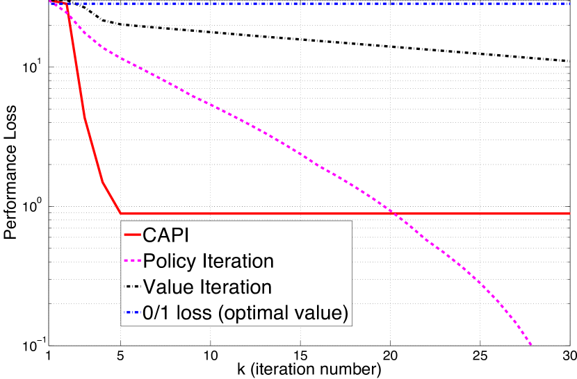
Figure 2: (1D Chain Walk with Policy Approximation Error) Performance loss for CAPI, Value Iteration, Policy Iteration, and the $0/1$-loss given $Q^{*}$.

We compare CAPI with Value Iteration (VI), Policy Iteration (PI), and a modified CAPI that uses the $0/1$-loss on a simple 1D chain walk problem (based on the example in Section 9.1 of Lagoudakis and Parr [43]). The problem has $200$ states, the reward function is zero everywhere except at states $10-15$ (where it is $+1$ for both actions) and $180-190$ (where it is $+0.1$ for both actions), and $\gamma=0.99$.

Note that the model is known. CAPI is run with the distribution $\nu_{n}$ in the loss function (1) as the uniform distribution over states. The value of $\hat{Q}^{\pi_{k}}$ at iteration $k$ of CAPI is obtained by running just one iteration of VI-based policy evaluation, i.e., $\hat{Q}^{\pi_{k}}=T^{\pi_{k}}\hat{Q}^{\pi_{k-1}}$, in which $T^{\pi_{k}}$ is the Bellman operator for policy $\pi_{k}$. This makes the number of times CAPI queries the model similar to that of VI. The policy space $\Pi$ is defined as the space of indicator functions of the set of all half-spaces, i.e., the set of policies that choose action $1$ (or $2$) on $\{1,\dotsc,p\}$ and action $2$ (or $1$) on $\{p+1,\dotsc,200\}$ for $1\leq p\leq 200$. This is a very small subset of all possible policies. We intentionally designed the reward function such that the optimal policy is not in $\Pi$, so CAPI will be subjected to policy approximation error.

Figure 2 shows that the performance loss of CAPI converges to this policy approximation error, which is the best solution achievable given $\Pi$. The convergence rate is considerably faster than that of VI and PI. This speedup is due to the fact that CAPI searches in a much smaller policy space compared to VI or PI. The comparison of CAPI and VI is especially striking, since both of them use the same number of queries to the model and are computationally comparable (CAPI is a bit more expensive than VI due to the optimization involved in finding the best policy in the policy space, but since the policy space is rather small in this problem, the difference is not considerable). The computation time of PI is considerably higher as it evaluates a policy at each iteration.

We also report the performance loss of a modified CAPI that uses the $0/1$-loss and the exact $Q^{*}$ (so there will be no estimation error). The result is quite poor. To understand this behaviour, note that the minimizer of the $0/1$-loss is a policy that approximates the greedy policy (in this case, the optimal policy) without paying attention to the action-gap function. Here, the minimizer of the $0/1$-loss policy is such that it fits the optimal policy, which does not belong to the policy space, in a large region of the state space where the action-gap is small and differs from the optimal policy in a smaller region where the action-gap is large. This selection ignores the relative importance of choosing the wrong action in different regions of the state space and results in poor behaviour (cf. Theorems 3–4 of [47]).

We now study the case in which the optimal policy belongs to policy space $\Pi$. We use the same 1D chain walk, with the difference that the reward function is zero everywhere except at states $10-15$ (where it is $+1$ for both actions). In the previous experiment, the reward function was also nonzero between $180-190$. Other than this, the experiment is performed as before. This change ensures that the optimal policy belongs to policy space $\Pi$.

The result is shown in Figure 3. The performance loss of both CAPI and PI goes to zero very quickly. However, the computation time of CAPI is comparable to VI, and is much cheaper than that of PI. The performance loss of the $0/1$-loss CAPI with the optimal action-value function is zero in this case, so we do not report it.

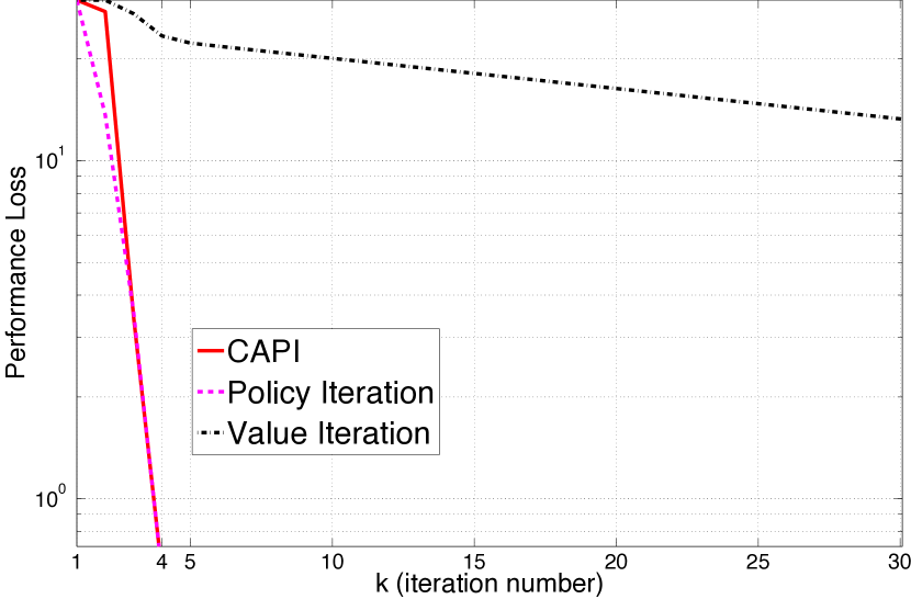
Figure 3: (1D Chain Walk without Policy Approximation Error) Performance loss for CAPI, Value Iteration, and Policy Iteration. After the $4^{\text{th}}$ iteration, the performance loss of PI and CAPI is zero.

V-B HIV drug schedule

Most of the anti-HIV drugs currently available fall into one of two categories: reverse transcriptase inhibitors (RTI) and protease inhibitors (PI). RTI and PI drugs act differently on the organism, and typical HIV treatments use drug cocktails containing both types of medication. Despite the success of drug cocktails in maintaining low viral loads, there are several complications associated with their long-term use. This has attracted the interest of the scientific community to the problem of optimizing drug-scheduling strategies. Among them, a strategy that has received a lot of attention recently is structured treatment interruption (STI), in which patients undergo alternate cycles with and without the drugs.

The scheduling of STI treatments can be seen as a sequential decision problem in which the actions correspond to the types of cocktail that should be administered to a patient [22]. To simplify the problem formulation, it is assumed that RTI and PI drugs are administered at fixed amounts, reducing the available actions to the four possible combinations of drugs. The goal is to minimize the HIV viral load using a drug amount as small as possible.

We studied the problem of optimizing STI treatments using a model of the interaction between the immune system and HIV developed by Adams et al. [1] based on real clinical data. All the parameters of the model were set as suggested by Ernst et al. [22]. The methodology adopted in the computational experiments, such as the evaluation of the decision policies and the collection of sample transitions, also followed the same protocol.

To illustrate the potential benefits of controlling the complexity of the decision policies, we compare the pure value-based algorithm adopted by Ernst et al. [22], Fitted Q-Iteration, with a modified version in which the space of policies is restricted. Following the original experiments, we approximated the value function using an ensemble of $30$ decision trees generated by Geurts et al.’s 2006 extra-trees algorithm (we refer to this instantiation of Fitted Q-Iteration as Tree-FQI). Tree-CAPI works exactly as Tree-FQI, except that instead of using the greedy policies induced by the current value function approximation, it uses a second ensemble of $30$ trees to represent the decision policies.

Note that in order to build the trees representing decision policies, the extra-trees algorithm has to be slightly modified to incorporate the estimated action-gap as its loss function. Consider a Tree-CAPI policy based on a single tree. The tree defines a partition ${\mathcal{X}}_{1},{\mathcal{X}}_{2},\dotsc$ of the state space. This partitioning of the state space defines a policy as described in Section III. When we have several trees, as in extra-trees, their policies are combined by voting to obtain the outcome policy.

The complexity of the models built by the extra-trees algorithm can be controlled by the minimum number of points required to split a node during the construction of the trees, $\eta$ [34]. In general, the larger this number is, the simpler the resulting models are. Here, we fixed this parameter for the trees representing the value function at $\eta_{\mathrm{v}}=50$, while the corresponding parameter for the decision-policy trees, called here $\eta_{\mathrm{\pi}}$, was varied in the set $\{2,10,20,50,100,200,300,500,1000,2000\}$.

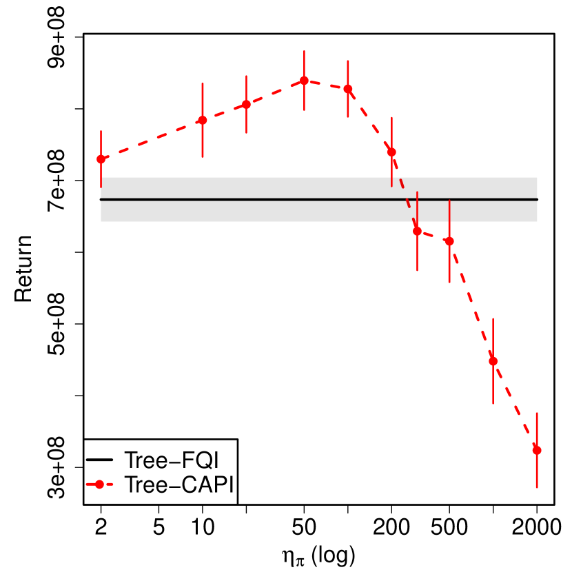
Figure 4: (HIV) Comparing the expected return for Tree-based CAPI vs. Tree-based Fitted Q-Iteration as a function of parameter $\eta_{\pi}$ describing the complexity of policy space (inversely proportional). The decision policies (in this case, STI treatments) were evaluated for $5,000$ days starting from an “unhealthy” state with a high viral load (see [22]). The error bars and shadowed region show one standard error over 50 runs.

Figure 4 shows the result of this an experiment. As can be seen, restricting the policy space can have a dramatic impact on the performance of the resulting decision policies. When $2\leq\eta_{\mathrm{\pi}}\leq 100$, the policies computed by Tree-CAPI perform better than those computed by Tree-FQI, leading to increases in the empirical return as high as $24\%$. On the other hand, an overly restricted policy space precludes the representation of the intricacies of an efficient STI treatment, resulting in poor performance. We expect these results to be representative of a more general trend, in which the “right” level of complexity of the decision policies is influenced by factors such as the difficulty of the problem and the number of sample transitions available. With CAPI, it is possible to adjust the complexity of the policy space to a specific context, and the use of a greedy policy is simply the particular case in which no restrictions are imposed.

VI Comparison with Other Work

As mentioned already, the most similar approach to CAPI is DPI [45], which uses rollouts. DPI-Critic [33], which is also a special case of CAPI, can benefit from value function regularities, but only in the correction term of the rollout estimates, for which DPI-Critic uses a general value function estimator to reduce the truncation bias. Both of these algorithms are special cases of CAPI with a particular choice for the policy evaluation step. The theoretical analysis for CAPI compared to that of DPI/DPI-Critic shows a tighter upper bound for the estimation error (e.g., $O(d\log(n)/n)$ for CAPI vs. $O(\sqrt{d/n})$ for DPI/DPI-Critic, for policy spaces of VC-dimension $d$), handles nonparametric policy spaces, and shows that solving MDPs with a favourable action-gap property is easier. In some other experiments reported in Appendix D, CAPI used orders of magnitude fewer samples than Tree-DPI to achieve good performance. This shows the power of generalizing with a good value function estimator.

Another similar approach is the Conservative Policy Iteration (CPI) algorithm introduced by Kakade and Langford [40]. CPI was designed to address the well-known problem that API may not converge, and thus the performance of the resulting policy may oscillate. CPI guarantees that the performance loss of the generated sequence of policies is monotonically decreasing before the algorithm stops (with high probability). DPI and CAPI do not have such a monotonicity guarantee (but note that we still have upper bounds on the performance loss). Recently Ghavamzadeh and Lazaric [36] have closely compared CPI and DPI, and concluded that these algorithms are actually quite similar (and as a result, CPI has some similarities with CAPI as well). One difference is in the probability distribution used in the minimization problem (3) for DPI. Also, CPI updates policies conservatively, but DPI does not. The effect of this conservatism is that CPI requires exponentially more iterations (and samples) than DPI (and, by extension, CAPI) to achieve the same accuracy. Also, the number of required iterations for DPI is a function of $1/(1-\gamma)$, which can be large for $\gamma$ close to $1$. Note that CPI might converge to a suboptimal policy whose performance is not better than the one achieved by DPI. For more details, we refer the reader to Ghavamzadeh and Lazaric [36].

There is an interesting connection between CAPI and the actor-critic (AC) family of algorithms [42, 51, 12]. The critic is essentially a policy evaluation algorithm, which is a component of CAPI too. On the other hand, in most implementations of AC algorithms, the actor uses a gradient-based approach to update the policy. If the actor was generated to minimize the loss function (1) in a policy space $\Pi$, one would obtain a CAPI-style algorithm.

An example of this relaxed definition of AC is a Fitted Q-Iteration algorithm developed by Antos et al. [2] that is tailored to continuous action spaces. The authors mentioned that the resulting method might be called a fitted actor-critic algorithm. That algorithm shares the general form of the actor with CAPI, but is specialized to a particular class of parametric Fitted Q-Iteration-based critics. Since these two algorithms consider different problems (continuous vs. finite action spaces), a direct comparison of their theoretical guarantees is not possible. Acknowledging this major difference, we remark that our analysis allows nonparametric policy spaces, while their analysis is specialized to parametric spaces. Moreover, their rate appears to be slower than what could be achieved. The reason is that they use global measures of complexity (pseudo-dimension, which is closely related to VC-dimension) and control the supremum of empirical processes as opposed to the more advanced techniques of this paper, i.e., localized Rademacher-based analysis (which is based on the modulus of continuity of the empirical process). On the other hand, they assume that the input data is a $\beta$-mixing process, which is more relaxed than our i.i.d. assumption.

The action-gap function and a similar notion of regularity have also been used by Dimitrakakis and Lagoudakis [18] in the context of rollout allocation. Their goal is to decide how to efficiently assign rollouts to states, so that informative samples can be provided to the classifier with as few rollouts as possible. The main idea is that it is easy to quickly choose the greedy action with high confidence when the action-gap function is large and vice versa. However, they do not consider the fine balance between large action-gap/small probability of error and small action-gap/small regret (they only consider the first aspect). Also, their suggested algorithm is based on the $0/1$-loss, which as argued before, can lead to bad policies.

VII Conclusion and Future Work

We proposed CAPI, a general family of algorithms that exploits regularities of both the value function and the policy. CAPI uses any policy evaluation method, defines an action-gap-weighted loss function, and finds the policy minimizing this loss from a desired policy space. We provided an error upper bound that is tighter than existing results and applies to general policy evaluation algorithms and nonparametric policy spaces.

Our experiments showed that when a powerful policy evaluation method such as Fitted Q-Iteration is used in CAPI, the resulting policy outperforms a purely value-based approach in terms of the quality of the solution and the sample efficiency. Moreover, our experiments in the appendix showed that CAPI outperforms a rollout-based classification-based RL algorithm.

CAPI might be computationally more expensive than a pure value-based approach. Its computational cost mainly depends on how the optimization problem (1) is solved. For example, the computational cost of learning a policy by Tree-CAPI is almost twice the cost of Tree-FQI, while the cost of finding the action is almost the same. We envision CAPI as being especially useful in the batch setting and for problems in which acquiring samples is expensive (such as in medical treatment design or mining optimization applications), so sample efficiency is more important than the computational complexity.

We showed how to efficiently solve the optimization problem (1) for policy spaces induced by local methods such as Decision Trees or KNN. Extending this to other reasonably general classes of policy spaces (e.g., policies that are defined by the sign of linear combination of basis functions) is an open question. The use of surrogate losses is likely to be a reasonable answer, but the theoretical properties of that approach should be investigated, possibly similar to what Bartlett et al. [8] do in the context of classification. Additionally, an interesting research direction is to extend and analyze CAPI for continuous action spaces.

The sampling distribution $\nu$ can have a big effect on the performance; how to choose it well is an open question. One could even change the sampling distribution at each iteration, to actively obtain more informative samples.

Finally, CAPI-style algorithms could be very useful in problems where the policy space needs to be restricted, by imposing constraints (e.g., torques not exceeding maximum values). Studying such applications would be interesting.

Appendix A Concentration Inequalities

For the convenience of the reader, we quote Bernstein inequality and Theorem 3.3 of Bartlett et al. [7].

Lemma 3 (Bernstein inequality – Theorem 6.12 of Steinwart and Christmann [56]).

Let $(\Omega,\mathcal{A},P)$ be a probability space, $B>0$, and $\sigma>0$ be real numbers, and $n\geq 1$ be an integer. Furthermore, let $X_{1},\dotsc,X_{n}:\Omega\to\mathbb{R}$ be independent random variables satisfying ${\mathbb{E}}\left[X_{i}\right]=0$, $\left\|X_{i}\right\|_{\infty}\leq B$, and ${\mathbb{E}}\left[X_{i}^{2}\right]\leq\sigma^{2}$ for all $i=1,2,\dotsc,n$. Then we have ${\mathbb{P}}\left\{\frac{1}{n}\sum_{i=1}^{n}X_{i}\geq\sqrt{\frac{2\sigma^{2}z}{n}}+\frac{2Bz}{3n}\right\}\leq e^{-z}$ $(z>0)$.

Theorem 4 (Theorem 3.3 of Bartlett et al. [7] – First Part).

Let ${\mathcal{F}}$ be a class of functions with ranges in $[a,b]$ and assume that there are some functional $T:{\mathcal{F}}\to\mathbb{R}^{+}$ and some constant $B$ such that for every $f\in{\mathcal{F}}$, ${\mathrm{Var}}\left[f\right]\leq T(f)\leq B{\mathbf{P}}f$. Let $\Psi$ be a sub-root function and let $r^{*}$ be the fixed point of $\Psi$. Assume that for any $r\geq r^{*}$, $\Psi$ satisfies $\Psi(r)\geq B{\mathbb{E}}\left[R_{n}\{f\in{\mathcal{F}}:T(f)\leq r\}\right]$. Then with $c_{1}=704$ and $c_{2}=26$, for any $K>1$ and every $x>0$, with probability at least $1-e^{-x}$, for any $f\in{\mathcal{F}}$, we have

$${\mathbf{P}}f\leq\frac{K}{K-1}{\mathbf{P}}_{n}f+\frac{c_{1}K}{B}r^{*}+\frac{x(11(b-a)+c_{2}BK)}{n}.$$

Appendix B Proof of the Main Result

Recall that the goal is to provide an upper bound for the loss $L({\hat{\pi}}_{n})$, where ${\hat{\pi}}_{n}$ is the minimizer of the distorted empirical loss function $\hat{L}_{n}$ obtained at each iteration (cf. (3)). The loss function $\hat{L}_{n}$, however, is defined based on the estimate ${\hat{Q}^{\pi^{\prime}}}$ instead of the true action-value function ${Q^{\pi^{\prime}}}$. This causes some errors. So in Lemma 5, we quantify how well ${\hat{\pi}}_{n}$ minimizes the loss function $L_{n}$ (defined based on ${Q^{\pi^{\prime}}}$ and unavailable to the algorithm). Having this result, we prove Theorem 1, which upper bounds the true loss $L({\hat{\pi}}_{n})$.

Lemma 5 (Loss Distortion Lemma).

Fix a policy $\pi^{\prime}$. Suppose that ${\hat{Q}^{\pi^{\prime}}}$ is an approximation of the action-value function ${Q^{\pi^{\prime}}}$. Given the dataset $\mathcal{D}_{n}$, let ${\hat{\pi}}_{n}$ be defined as (3) and define $\pi^{*}_{n}\leftarrow\mathop{\textrm{argmin}}_{\pi\in\Pi}L_{n}(\pi)$. Let Assumption II-B hold. There exist finite $c_{1},c_{2}>0$, which depend only on $\zeta$, $c_{g}$, and $Q_{\textrm{max}}$, such that for any $z>0$, we have

$$L_{n}(\hat{\pi}_{n})\leq 3L_{n}(\pi^{*}_{n})+c_{1}\left\|{\hat{Q}^{\pi^{\prime}}}-{Q^{\pi^{\prime}}}\right\|_{\infty,\mathcal{D}_{n}}^{1+\zeta}+c_{2}\frac{z}{n},$$

with probability at least $1-e^{-z}$.

This lemma states that the empirical loss $L_{n}$ of policy ${\hat{\pi}}_{n}$, which is the minimizer of the distorted empirical loss $\hat{L}_{n}$, is still close to the true minimizer of $L_{n}$, which uses the true, but unavailable, action-value value function ${Q^{\pi^{\prime}}}$. The difference mainly depends on the error of estimating ${Q^{\pi^{\prime}}}$ by ${\hat{Q}^{\pi^{\prime}}}$. When the problem has a favourable action-gap regularity (i.e., $\zeta>0$), the error is exponentially dampened by a factor of $1+\zeta$. This lemma currently uses the supremum norm of the policy evaluation error, but one might also extend it to an $L_{p}$-norm result similar to what was done by Farahmand [23]. Note that even though the proof technique here has some similarities with the proofs by [23], they are considerably different.

In the proofs, $c_{1},c_{2},\dotsc$ are constants whose values may change from line to line – unless specified otherwise.

Proof of Lemma 5.

Let $\varepsilon=\|{\hat{Q}^{\pi^{\prime}}}-{Q^{\pi^{\prime}}}\|_{\infty,\mathcal{D}_{n}}$ and define the set $A_{\varepsilon}=\{x:0<{\mathbf{g}_{Q^{\pi^{\prime}}}}(x)\leq 4\varepsilon\}$. Denote $p={\mathbb{P}}_{\nu}\left(X\in A_{\varepsilon}\right)$. For any $z>0$, Bernstein inequality (Lemma 3 in Appendix A) shows that ${\mathbb{P}}_{\nu_{n}}\left(X\in A_{\varepsilon}\right)-{\mathbb{P}}_{\nu}\left(X\in A_{\varepsilon}\right)\leq\sqrt{\frac{2p(1-p)z}{n}}+\frac{2z}{3n}$ with probability at least $1-e^{-z}$. By the arithmetic mean–geometric mean inequality $\sqrt{[p(1-p)]\frac{2z}{n}}\leq\frac{p(1-p)}{2}+\frac{2z}{2n}\leq\frac{p}{2}+\frac{z}{n}$, so we get

$${\mathbb{P}}_{\nu_{n}}\left(X\in A_{\varepsilon}\right)\leq\frac{3}{2}{\mathbb{P}}_{\nu}\left(X\in A_{\varepsilon}\right)+\frac{5z}{3n}$$ (5)

with probability at least $1-e^{-z}$. From now on, we focus on the event that this inequality holds.

Define the new auxiliary loss $\tilde{L}_{n}(\pi)=\int_{{\mathcal{X}}}{\mathbf{g}_{Q^{\pi^{\prime}}}}(x){\mathbb{I}}{\{\pi(x)\neq\mathop{\textrm{argmax}}_{a\in{\mathcal{A}}}{\hat{Q}^{\pi^{\prime}}}(x,a)\}}\mathrm{d}\nu_{n}$. Notice that unlike $\hat{L}_{n}(\pi)$, it uses the weighting function ${\mathbf{g}_{Q^{\pi^{\prime}}}}$ (instead of ${\mathbf{g}_{\hat{Q}^{\pi^{\prime}}}}$). In the following, for any $\pi$, we first relate $L_{n}(\pi)$ to $\tilde{L}_{n}(\pi)$, and then relate $\tilde{L}_{n}(\pi)$ to $\hat{L}_{n}(\pi)$.

Upper bounding $|L_{n}(\pi)-\tilde{L}_{n}(\pi)|$. For any $\pi$,

$$\left|L_{n}(\pi)-\tilde{L}_{n}(\pi)\right|=$$

$$\Bigg{|}\int_{\mathcal{X}}{\mathbf{g}_{Q^{\pi^{\prime}}}}(x)\Big{[}{\mathbb{I}}{\{\pi(x)\neq\mathop{\textrm{argmax}}_{a\in{\mathcal{A}}}{Q^{\pi^{\prime}}}(x,a)\}}-{}$$

$$\qquad\qquad\qquad{\mathbb{I}}{\{\pi(x)\neq\mathop{\textrm{argmax}}_{a\in{\mathcal{A}}}{\hat{Q}^{\pi^{\prime}}}(x,a)\}}\Big{]}\mathrm{d}\nu_{n}\Bigg{|}$$

$$\leq\int_{\mathcal{X}}{\mathbf{g}_{Q^{\pi^{\prime}}}}(x){\mathbb{I}}{\{\mathop{\textrm{argmax}}_{a\in{\mathcal{A}}}{Q^{\pi^{\prime}}}(x,a)\neq\mathop{\textrm{argmax}}_{a\in{\mathcal{A}}}{\hat{Q}^{\pi^{\prime}}}(x,a)\}}\mathrm{d}\nu_{n}$$

$$=\int_{A_{\varepsilon}}{\mathbf{g}_{Q^{\pi^{\prime}}}}(x){\mathbb{I}}{\{\mathop{\textrm{argmax}}_{a\in{\mathcal{A}}}{Q^{\pi^{\prime}}}(x,a)\neq\mathop{\textrm{argmax}}_{a\in{\mathcal{A}}}{\hat{Q}^{\pi^{\prime}}}(x,a)\}}\mathrm{d}\nu_{n}$$

$${}+\int_{A^{c}_{\varepsilon}}{\mathbf{g}_{Q^{\pi^{\prime}}}}(x){\mathbb{I}}{\{\mathop{\textrm{argmax}}_{a\in{\mathcal{A}}}{Q^{\pi^{\prime}}}(x,a)\neq\mathop{\textrm{argmax}}_{a\in{\mathcal{A}}}{\hat{Q}^{\pi^{\prime}}}(x,a)\}}\mathrm{d}\nu_{n}.$$

Whenever $|{\hat{Q}^{\pi^{\prime}}}(x,a)-{Q^{\pi^{\prime}}}(x,a)|<\frac{1}{2}{\mathbf{g}_{Q^{\pi^{\prime}}}}(x)$ (for $x\in\mathcal{D}_{n}$ and $a\in\{1,2\}$), the maximizer action is the same. So on the set $A_{\varepsilon}^{c}$, where ${\mathbf{g}_{Q^{\pi^{\prime}}}}(x)>4\varepsilon\geq 4|{\hat{Q}^{\pi^{\prime}}}(x,a)-{Q^{\pi^{\prime}}}(x,a)|$, the value of ${\mathbb{I}}{\{\mathop{\textrm{argmax}}_{a\in{\mathcal{A}}}{Q^{\pi^{\prime}}}(x,a)\neq\mathop{\textrm{argmax}}_{a\in{\mathcal{A}}}{\hat{Q}^{\pi^{\prime}}}(x,a)\}}$ is always zero. Thus for any $z>0$, we have

$$\left|L_{n}(\pi)-\tilde{L}_{n}(\pi)\right|\leq(4\varepsilon){\mathbb{P}}_{\nu_{n}}\left(X\in A_{\varepsilon}\right)\leq$$

$$4\varepsilon\left[\frac{3}{2}{\mathbb{P}}_{\nu}\left(X\in A_{\varepsilon}\right)+\frac{5z}{3n}\right]\leq$$

$$6\times 2^{2\zeta}\left\|{\hat{Q}^{\pi^{\prime}}}-{Q^{\pi^{\prime}}}\right\|_{\infty,\mathcal{D}_{n}}^{1+\zeta}+\frac{20}{3}\left\|{\hat{Q}^{\pi^{\prime}}}-{Q^{\pi^{\prime}}}\right\|_{\infty,\mathcal{D}_{n}}\frac{z}{n}$$

$$\leq c_{1}(\zeta)\left\|{\hat{Q}^{\pi^{\prime}}}-{Q^{\pi^{\prime}}}\right\|_{\infty,\mathcal{D}_{n}}^{1+\zeta}+c_{2}(Q_{\textrm{max}})\frac{z}{n}.$$ (6)

Here we used (5) in the second inequality, Assumption II-B in the third inequality, and $\|{\hat{Q}^{\pi^{\prime}}}-{Q^{\pi^{\prime}}}\|_{\infty,\mathcal{D}_{n}}\leq 2Q_{\textrm{max}}$ in the last one.

Relation of $\hat{L}_{n}(\pi)$ to $\tilde{L}_{n}(\pi)$. First note that $|{\mathbf{g}_{\hat{Q}^{\pi^{\prime}}}}(x)-{\mathbf{g}_{Q^{\pi^{\prime}}}}(x)|\leq 2\varepsilon$ (for all $x\in\mathcal{D}_{n}$). We also have

$$\max_{x\in A_{\varepsilon}^{c}\cap\mathcal{D}_{n}}\frac{{\mathbf{g}_{\hat{Q}^{\pi^{\prime}}}}(x)-{\mathbf{g}_{Q^{\pi^{\prime}}}}(x)}{{\mathbf{g}_{Q^{\pi^{\prime}}}}(x)}\leq\frac{2\varepsilon}{4\varepsilon}=\frac{1}{2},$$

$$\max_{x\in A_{\varepsilon}^{c}\cap\mathcal{D}_{n}}\frac{{\mathbf{g}_{Q^{\pi^{\prime}}}}(x)-{\mathbf{g}_{\hat{Q}^{\pi^{\prime}}}}(x)}{{\mathbf{g}_{\hat{Q}^{\pi^{\prime}}}}(x)}\leq\frac{2\varepsilon}{2\varepsilon}=1.$$

Thus,

$$\hat{L}_{n}(\pi)-\tilde{L}_{n}(\pi)=$$

$$\int_{A_{\varepsilon}}({\mathbf{g}_{\hat{Q}^{\pi^{\prime}}}}(x)-{\mathbf{g}_{Q^{\pi^{\prime}}}}(x)){\mathbb{I}}{\{\pi(x)\neq\mathop{\textrm{argmax}}_{a\in{\mathcal{A}}}{\hat{Q}^{\pi^{\prime}}}(x,a)\}}\mathrm{d}\nu_{n}+{}$$

$$\int_{A_{\varepsilon}^{c}}\frac{{\mathbf{g}_{\hat{Q}^{\pi^{\prime}}}}(x)-{\mathbf{g}_{Q^{\pi^{\prime}}}}(x)}{{\mathbf{g}_{Q^{\pi^{\prime}}}}(x)}{\mathbf{g}_{Q^{\pi^{\prime}}}}(x){\mathbb{I}}{\{\pi(x)\neq\mathop{\textrm{argmax}}_{a\in{\mathcal{A}}}{\hat{Q}^{\pi^{\prime}}}(x,a)\}}\mathrm{d}\nu_{n}$$

$${}\leq{}(2\varepsilon){\mathbb{P}}_{\nu_{n}}\left(X\in A_{\varepsilon}\right)+\frac{1}{2}\tilde{L}_{n}(\pi).$$

After re-arranging, we get

$$\hat{L}_{n}(\pi)\leq\frac{3}{2}\tilde{L}_{n}(\pi)+2\varepsilon\,{\mathbb{P}}_{\nu_{n}}\left(X\in A_{\varepsilon}\right).$$ (7)

Likewise, by writing ${\mathbf{g}_{Q^{\pi^{\prime}}}}(x)-{\mathbf{g}_{\hat{Q}^{\pi^{\prime}}}}(x)$ as $\frac{{\mathbf{g}_{Q^{\pi^{\prime}}}}(x)-{\mathbf{g}_{\hat{Q}^{\pi^{\prime}}}}(x)}{{\mathbf{g}_{\hat{Q}^{\pi^{\prime}}}}(x)}{\mathbf{g}_{\hat{Q}^{\pi^{\prime}}}}(x)$ and doing a similar decomposition of the state space into $A_{\varepsilon}$ and $A_{\varepsilon}^{c}$, we get

$$\hat{L}_{n}(\pi)\geq\frac{1}{2}\tilde{L}_{n}(\pi)-\varepsilon{\mathbb{P}}_{\nu_{n}}\left(X\in A_{\varepsilon}\right).$$ (8)

We use the optimizer property of $\hat{\pi}_{n}$ (which implies that $\hat{L}_{n}(\hat{\pi}_{n})\leq\hat{L}_{n}(\pi^{*}_{n})$), apply (7), and finally use inequalities (B) and (5) to get

$$\hat{L}_{n}(\hat{\pi}_{n}) \leq\hat{L}_{n}(\pi^{*}_{n})\leq\frac{3}{2}\tilde{L}_{n}(\pi^{*}_{n})+(2\varepsilon){\mathbb{P}}_{\nu_{n}}\left(X\in A_{\varepsilon}\right)$$

$$\leq{}\frac{3}{2}\left[L_{n}(\pi^{*}_{n})+c_{1}\left\|{\hat{Q}^{\pi^{\prime}}}-{Q^{\pi^{\prime}}}\right\|_{\infty,\mathcal{D}_{n}}^{1+\zeta}+c_{2}\frac{z}{n}\right]+{}$$

$$\quad\,(2\varepsilon)\left[\frac{3}{2}{\mathbb{P}}_{\nu}\left(X\in A_{\varepsilon}\right)+\frac{5}{3}\frac{z}{n}\right].$$

From (8) and by applying (B), we also have

$$\hat{L}_{n}(\hat{\pi}_{n}) \geq\frac{1}{2}\tilde{L}_{n}(\hat{\pi}_{n})-\varepsilon\,{\mathbb{P}}_{\nu_{n}}\left(X\in A_{\varepsilon}\right)$$

$$\geq\frac{1}{2}\left[L_{n}({\hat{\pi}}_{n})-c_{1}\left\|{\hat{Q}^{\pi^{\prime}}}-{Q^{\pi^{\prime}}}\right\|_{\infty,\mathcal{D}_{n}}^{1+\zeta}-c_{2}\frac{z}{n}\right]-{}$$

$$\quad\;\;\varepsilon\left[\frac{3}{2}{\mathbb{P}}_{\nu}\left(X\in A_{\varepsilon}\right)+\frac{5z}{3n}\right].$$

These two inequalities imply that $L_{n}({\hat{\pi}}_{n})\leq 3L_{n}(\pi^{*}_{n})+c_{1}\|{\hat{Q}^{\pi^{\prime}}}-{Q^{\pi^{\prime}}}\|_{\infty,\mathcal{D}_{n}}^{1+\zeta}+c_{2}\frac{z}{n}$ in the event that (5) holds, which has probability at least $1-e^{-z}$. ∎

Proof of Theorem 1.

We use Theorem 3.3 by Bartlett et al. [7] (quoted as Theorem 4 in Appendix A). For function $l(\pi)(x)={\mathbf{g}_{Q^{\pi^{\prime}}}}(x){\mathbb{I}}{\{\pi(x)\neq\mathop{\textrm{argmax}}_{a\in{\mathcal{A}}}{Q^{\pi^{\prime}}}(x,a)\}}$, we have

$${\mathrm{Var}}\left[l(\pi)(X)\right] \leq{\mathbb{E}}\left[\left|{\mathbf{g}_{Q^{\pi^{\prime}}}}(X){\mathbb{I}}{\{\pi(X)\neq\mathop{\textrm{argmax}}_{a\in{\mathcal{A}}}{Q^{\pi^{\prime}}}(X,a)\}}\right|^{2}\right]$$

$$\leq 2Q_{\textrm{max}}{\mathbb{E}}\left[l(\pi)(X)\right],$$

so the variance condition of that theorem is satisfied. If we have a function $\Psi$ as defined in (4), the theorem states that there exist $c_{1},c_{2}>0$ such that for any $z>0$ and any $\pi\in\Pi$ (including ${\hat{\pi}}_{n}\in\Pi$),

$$L(\pi)={\mathbf{P}}l(\pi)\leq 2P_{n}l(\pi)+c_{1}r^{*}+c_{2}\frac{z}{n},$$ (9)

with probability at least $1-e^{-z}$ ($c_{1}$ can be chosen as $704/Q_{\textrm{max}}$ and $c_{2}$ can be chosen as $126\,Q_{\textrm{max}}$).

Let ${\pi^{*}_{\Pi}}\leftarrow\mathop{\textrm{argmin}}_{\pi\in\Pi}L(\pi)$ be the minimizer of the expected loss in policy space $\Pi$. Consider (9) with the choice of $\pi={\hat{\pi}}_{n}$, and add and subtract $6P_{n}l({\pi^{*}_{\Pi}})$ and $6{\mathbf{P}}l({\pi^{*}_{\Pi}})$ and then use Lemma 5. With probability at least $1-2e^{-z}$, we get

$$L({\hat{\pi}}_{n})\leq{} 2{\mathbf{P}}_{n}l({\hat{\pi}}_{n})-6\left[{\mathbf{P}}_{n}l({\pi^{*}_{\Pi}})-{\mathbf{P}}_{n}l({\pi^{*}_{\Pi}})\right]$$

$${}-6\left[{\mathbf{P}}l({\pi^{*}_{\Pi}})-{\mathbf{P}}l({\pi^{*}_{\Pi}})\right]+c_{1}r^{*}+c_{2}\frac{z}{n}$$

$$\leq{} 6\left[{\mathbf{P}}_{n}l(\pi^{*}_{n})-{\mathbf{P}}_{n}l({\pi^{*}_{\Pi}})\right]+6\left[{\mathbf{P}}_{n}l({\pi^{*}_{\Pi}})-{\mathbf{P}}l({\pi^{*}_{\Pi}})\right]$$

$$+6{\mathbf{P}}l({\pi^{*}_{\Pi}})+c_{1}r^{*}+c_{2}\left\|{\hat{Q}^{\pi^{\prime}}}-{Q^{\pi^{\prime}}}\right\|_{\infty,\mathcal{D}_{n}}^{1+\zeta}+c_{3}\frac{z}{n}$$

$$\leq{} 6\left[{\mathbf{P}}_{n}l({\pi^{*}_{\Pi}})-{\mathbf{P}}l({\pi^{*}_{\Pi}})\right]+6{\mathbf{P}}l({\pi^{*}_{\Pi}})+c_{1}r^{*}$$

$${}+c_{2}\left\|{\hat{Q}^{\pi^{\prime}}}-{Q^{\pi^{\prime}}}\right\|_{\infty,\mathcal{D}_{n}}^{1+\zeta}+c_{3}\frac{z}{n},$$ (10)

where in the last inequality we used the minimizing property of $\pi^{*}_{n}$, i.e., ${\mathbf{P}}_{n}l(\pi^{*}_{n})-{\mathbf{P}}_{n}l({\pi^{*}_{\Pi}})\leq 0$. Here $c_{2}$ can be chosen as $36\times 2^{2\zeta}$.

To upper bound ${\mathbf{P}}_{n}l({\pi^{*}_{\Pi}})-{\mathbf{P}}l({\pi^{*}_{\Pi}})$, we apply Bernstein inequality (Lemma 3 in Appendix A) to get that for any $z>0$, ${\mathbf{P}}_{n}l({\pi^{*}_{\Pi}})-{\mathbf{P}}l({\pi^{*}_{\Pi}})\leq\sqrt{\frac{2{\mathrm{Var}}\left[l({\pi^{*}_{\Pi}})\right]z}{n}}+\frac{4Q_{\textrm{max}}z}{3n}$, with probability at least $1-e^{-z}$. Since ${\mathrm{Var}}\left[l({\pi^{*}_{\Pi}})\right]\leq 2Q_{\textrm{max}}{\mathbf{P}}l({\pi^{*}_{\Pi}})$ (as shown above), by the application of arithmetic mean–geometric mean inequality we obtain ${\mathbf{P}}_{n}l({\pi^{*}_{\Pi}})-{\mathbf{P}}l({\pi^{*}_{\Pi}})\leq{\mathbf{P}}l({\pi^{*}_{\Pi}})+\frac{7Q_{\textrm{max}}z}{3n}$ with the same probability. This and (10) result in

$$L({\hat{\pi}}_{n})\leq 12{\mathbf{P}}l({\pi^{*}_{\Pi}})+c_{1}r^{*}+c_{2}\left\|{\hat{Q}^{\pi^{\prime}}}-{Q^{\pi^{\prime}}}\right\|_{\infty,\mathcal{D}_{n}}^{1+\zeta}+c_{3}\frac{z}{n},$$

with probability at least $1-3e^{-z}$ as desired. ∎

Proof of Theorem 2.

It is shown by [45] that

$$V^{*}-V^{\pi_{K}}\leq$$

$$\sum_{k=0}^{K-1}\gamma^{K-k-1}(\mathcal{P}^{\pi^{*}})^{K-k-1}\sum_{m\geq 0}\gamma^{m}(\mathcal{P}^{\pi_{k+1}})^{m}l^{\pi_{k}}(\pi_{k+1})$$

$$+(\gamma\mathcal{P}^{\pi^{*}})^{K}(V^{*}-V^{\pi_{0}}).$$

We apply $\rho$ to both sides and use the definition of $c_{\rho,\nu}(m_{1};m_{2};\pi)$ to get

$$\rho(V^{*}-V^{\pi_{K}})\leq$$

$$\sum_{k=0}^{K-1}\gamma^{K-k-1}\sum_{m\geq 0}\gamma^{m}c_{\rho,\nu}(K-k-1,m;\pi_{k+1})\,\nu l^{\pi_{k}}(\pi_{k+1})$$

$${}+\gamma^{K}(2Q_{\textrm{max}}).$$

Recall that $\nu l^{\pi_{k}}(\pi_{k+1})=L^{\pi_{k}}(\pi_{k+1})$. We decompose $\gamma$ to $\gamma^{s}\gamma^{(1-s)}$ (for $0\leq s\leq 1$) and separate terms involving the concentrability coefficients and those related to $L^{\pi_{k}}(\pi_{k+1})$. We then have for any $0\leq s\leq 1$,

$$\rho(V^{*}-V^{\pi_{K}})\leq$$

$$\max_{0\leq k\leq K-1}\left[\gamma^{s(K-k-1)}L^{\pi_{k}}(\pi_{k+1})\right]\times$$

$$\,\sum_{k^{\prime}=0}^{K-1}\gamma^{(1-s)k^{\prime}}\sum_{m\geq 0}\gamma^{m}\sup_{\pi^{\prime}\in\Pi}c_{\rho,\nu}(k^{\prime},m;\pi^{\prime})+\gamma^{K}(2Q_{\textrm{max}}).$$

Taking the infimum w.r.t. $s$ and using the definition of $C_{\rho,\nu}(K)$, we get that for $\mathrm{Loss}(\pi_{K};\rho)=\rho(V^{*}-V^{\pi_{K}})$,

$$\mathrm{Loss}(\pi_{K};\rho)\leq$$

$$\frac{2}{1-\gamma}\Big{[}\inf_{s\in[0,1]}C_{\rho,\nu}(K,s)\max_{0\leq k\leq K-1}[\gamma^{s(K-k-1)}L^{\pi_{k}}(\pi_{k+1})]$$

$$\qquad\quad{}+\gamma^{K}R_{\textrm{max}}\Big{]}.$$ (11)

Fix $0<\delta<1$. For each iteration $k=0,\dotsc,K-1$, by invoking Theorem 1 with the confidence parameter $\delta/K$, we get $L^{\pi_{k}}(\pi_{k+1})\leq 12\inf_{\pi\in\Pi}L^{\pi_{k}}(\pi)+c_{1}r^{*}+c_{2}\|\hat{Q}^{\pi_{k}}-Q^{\pi_{k}}\|_{\infty,\mathcal{D}_{n}^{k}}^{1+\zeta}+c_{3}\frac{\ln(K/\delta)}{n}$, which holds with probability at least $1-\delta/K$. Since $\inf_{\pi\in\Pi}L^{\pi_{k}}(\pi)\leq d(\Pi)$, the previous set of inequalities alongside (B) imply the desired result. ∎

We would like to remark that to extend the analysis to ${|{\mathcal{A}}|}>2$, Lemma 5 is the main result that should be modified. The proofs of Theorems 1 and 2 remain intact.

Appendix C Upper bound on $r^{*}$

The following proposition provides a distribution-free upper bound for $r^{*}$ (4) for policy space $\Pi$ with a finite VC-dimension. We closely follow the proof of Corollary 3.7 of Bartlett et al. [7].

Proposition 6.

Suppose that policy space $\Pi$ has a finite VC-dimension $d$. There exists constant $c>0$, which is independent of $n$ and $d$, such that for $n\geq d$, complexity condition (4) is satisfied with $r^{*}\leq\frac{cd\log(n/d)}{n}$.

Proof.

The proof has three main steps: 1) the Rademacher complexity of $\left\{\,l(\pi)\,:\,\pi\in\Pi,{\mathbf{P}}l^{2}(\pi)\leq r\,\right\}$ (the RHS of (4)) is upper bounded by the integral of the metric entropy (i.e., logarithm of the covering number), 2) the metric entropy of that set is related to the metric entropy of $\Pi$, and 3) the metric entropy of $\Pi$ is related to its VC-dimension.

1) Define the sub-root function $\Psi(r)=20Q_{\textrm{max}}{\mathbb{E}}\left[R_{n}\left\{\,l(\pi)\,:\,\pi\in\Pi,{\mathbf{P}}l^{2}(\pi)\leq r\,\right\}\right]+44Q_{\textrm{max}}^{2}\frac{\log n}{n}.$ If $r\geq\Psi(r)$, Corollary 2.2 of Bartlett et al. [7] indicates that with probability at least $1-1/n$, we have $\left\{\,l(\pi)\,:\,\pi\in\Pi,{\mathbf{P}}l^{2}(\pi)\leq r\,\right\}\subseteq\left\{\,l(\pi)\,:\,\pi\in\Pi,{\mathbf{P}}_{n}l^{2}(\pi)\leq 2r\,\right\}$. Thus, we can upper bound the Rademacher complexity of $\left\{\,l(\pi)\,:\,\pi\in\Pi,{\mathbf{P}}l^{2}(\pi)\leq r\,\right\}$ as ${\mathbb{E}}\left[R_{n}\left\{\,l(\pi)\,:\,\pi\in\Pi,{\mathbf{P}}l^{2}(\pi)\leq r\,\right\}\right]\leq{\mathbb{E}}\left[R_{n}\left\{\,l(\pi)\,:\,\pi\in\Pi,{\mathbf{P}}_{n}l^{2}(\pi)\leq 2r\,\right\}\right]+\frac{2Q_{\textrm{max}}}{n}.$ The fixed-point equation $r^{*}=\Psi(r^{*})$ satisfies

$$r^{*}\leq 20Q_{\textrm{max}}{\mathbb{E}}\left[R_{n}\left\{\,l(\pi)\,:\,\pi\in\Pi,{\mathbf{P}}_{n}l^{2}(\pi)\leq 2r^{*}\,\right\}\right]+$$

$$\frac{2Q_{\textrm{max}}+44Q_{\textrm{max}}^{2}\log n}{n}.$$ (12)

Using the metric entropy integral upper bound for the Rademacher complexity (Theorem A.7 of Bartlett et al. [7]; originally from Dudley [19]), we get that there exists a constant $C>0$ such that

$${\mathbb{E}}\left[R_{n}\left\{\,l(\pi)\,:\,\pi\in\Pi,{\mathbf{P}}_{n}l^{2}(\pi)\leq 2r^{*}\,\right\}\right]\leq$$

$$\frac{C}{\sqrt{n}}{\mathbb{E}}\left[\int_{0}^{\sqrt{2r^{*}}}\sqrt{\log{\mathcal{N}}(\varepsilon,\left\{\,l(\pi)\,:\,\pi\in\Pi\,\right\},L_{2}({\mathbf{P}}_{n}))}\;\mathrm{d}\varepsilon\right].$$

Here ${\mathcal{N}}(\varepsilon,\left\{\,l(\pi)\,:\,\pi\in\Pi\,\right\},L_{2}({\mathbf{P}}_{n}))$ is an $\varepsilon$-covering number of the set $\left\{\,l(\pi)\,:\,\pi\in\Pi\,\right\}$ w.r.t. the $L_{2}({\mathbf{P}}_{n})$-norm (cf. Chapter 9 of Györfi et al. [38]).

2) Since for any $\pi_{1}$ and $\pi_{2}$, we have $|l(x;\pi_{1})-l(x;\pi_{2})|^{2}\leq(2Q_{\textrm{max}})^{2}|{\mathbb{I}}{\{\pi_{1}(x)\neq\pi_{2}(x)\}}|^{2}$, a $u$-covering for $\Pi$ w.r.t. $L_{2}({\mathbf{P}}_{n})$ induces a $2Q_{\textrm{max}}u$-covering for $\left\{\,l(\pi)\,:\,\pi\in\Pi\,\right\}$. Therefore, ${\mathcal{N}}(\varepsilon,\left\{\,l(\pi)\,:\,\pi\in\Pi\,\right\},L_{2}({\mathbf{P}}_{n}))\leq{\mathcal{N}}(\frac{\varepsilon}{2Q_{\textrm{max}}},\Pi,L_{2}({\mathbf{P}}_{n}))$.

3) For a class $\Pi$ with finite VC-dimension $d$, its metric entropy can be upper bounded by $\log{\mathcal{N}}(\varepsilon,\Pi,L_{2}({\mathbf{P}}_{n}))\leq cd\log(1/\varepsilon)$ for some constant $c>0$. Thus,

$${\mathbb{E}}\left[R_{n}\left\{\,l(\pi)\,:\,\pi\in\Pi,{\mathbf{P}}_{n}l^{2}(\pi)\leq 2r^{*}\,\right\}\right]\leq$$

$$\sqrt{\frac{cdr^{*}\log(1/r^{*})}{n}}\leq\sqrt{c\left(\frac{d^{2}}{n^{2}}+\frac{dr^{*}\log(n/ed)}{n}\right)}.$$

Using this upper bound and solving for $r^{*}$ in (C) one get that for $n\geq d$, we have $r^{*}\leq\frac{cd\log(n/d)}{n}$. ∎

Appendix D Additional Experiments

We present some additional experiments to show that CAPI is a quite flexible framework and that the algorithms derived from it (by choosing PolicyEval and policy space $\Pi$) can be quite competitive.

The benchmark domains that we consider are Mountain-Car (2-dimensional state space) and Pole Balancing (4-dimensional state space) – both standard benchmarks in the reinforcement learning community. As a showcase of CAPI’s flexibility in the choice of the policy evaluation method and policy space $\Pi$, we use different algorithms for each domain.

D-A Mountain-Car

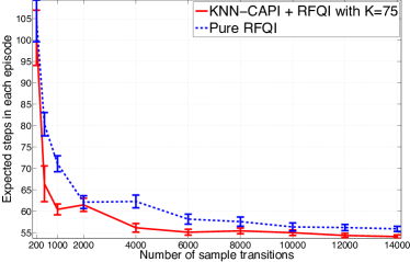
(a) Steps to goal

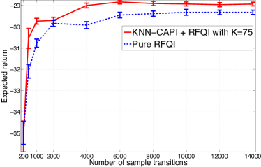
(b) Return

Figure 5: (Mountain-Car) Comparing the expected (a) number of steps to goal and (b) return in each episode for KNN-CAPI vs. Regularized Fitted Q-Iteration as a function of sample size. The error bars show one standard error over 50 runs.

We compare an instantiation of CAPI with a pure value-based approach on the Mountain-Car task [58], which has a 2-dimensional state space. The choice of value-based approach is the nonparametric kernelized Regularized Fitted Q-Iteration (RFQI) algorithm [26]. For CAPI, we have to choose the policy evaluation method PolicyEval and policy space $\Pi$ (cf. Algorithm 1). For a given policy $\pi_{k}$, we perform one iteration of RFQI (used for policy evaluation only, that is, there is no policy improvement) to estimate $\hat{Q}^{\pi_{k}}$. This is similar to how CAPI was implemented in the 1D Chain Walk example in Section V-A, except that here we deal with a continuous state space, so we use an approximate value iteration algorithm RFQI instead of the exact value iteration.

To derive $\pi_{k+1}$ from $\hat{Q}^{\pi_{k}}$, we use action-gap-weighted KNN-CAPI formulation as follows. At any state $x$, KNN-CAPI chooses an action that minimizes the CAPI’s empirical loss (1) in the $\kappa$-neighbourhood of $x$. More concretely, suppose that the state space ${\mathcal{X}}$ is endowed with a norm $\left\|\cdot\right\|$, e.g., the $l_{2}$-norm for ${\mathcal{X}}\subset\mathbb{R}^{d}$. For some positive integer $\kappa$, let $\mathrm{N}_{\kappa}(x)\subseteq\mathcal{D}_{n}^{(k)}$ be the set of $\kappa$-closest points to $x$ in $\mathcal{D}_{n}^{(k)}$ (w.r.t. the norm of ${\mathcal{X}}$), breaking ties deterministically. The KNN-based CAPI policy $\pi_{k+1}(x)$ is then defined as:

$$\pi_{k+1}(x)\leftarrow\mathop{\textrm{argmin}}_{a\in{\mathcal{A}}}\sum_{X_{i}\in\mathrm{N}_{\kappa}(x)}\mathbf{g}_{\hat{Q}^{\pi_{k}}}(X_{i}){\mathbb{I}}{\{a\neq{\hat{\pi}}(X_{i};\hat{Q}^{\pi_{k}})\}}$$

$$\equiv\mathop{\textrm{argmin}}_{a\in{\mathcal{A}}}\sum_{X_{i}\in\mathrm{N}_{\kappa}(x)}\hat{Q}^{\pi_{k}}(X_{i},{\hat{\pi}}(X_{i};\hat{Q}^{\pi_{k}}))-\hat{Q}^{\pi_{k}}(X_{i},a)$$

$$\equiv\mathop{\textrm{argmax}}_{a\in{\mathcal{A}}}\sum_{X_{i}\in\mathrm{N}_{\kappa}(x)}\hat{Q}^{\pi_{k}}(X_{i},a),$$

Similar to Tree-CAPI, this is a very simple rule: pick the action that maximizes the action-value at the data points in the $\kappa$-NN of the query point $x$. One could also assign different weights to each point in $\mathrm{N}_{\kappa}(x)$ as a function of distance to $x$, or more generally, use any local averaging estimator [17, 38] without much change in the formulation. The derivation of KNN-CAPI for ${|{\mathcal{A}}|}>2$ leads to the same rule.

We implemented the dynamics and the reward function of Mountain-Car task the same as Example 8.2 of Sutton and Barto [58], and we set the discount factor to $\gamma=0.98$. The initial state was chosen uniformly random and the data was collected by a uniformly random policy. For data collection, we used trajectories with the length of at most 100 steps (or if the episode is terminated by reaching the goal). To evaluate the policy, we let the agent go for at most 200 steps. If it did not reach the goal by then, 200 was reported as the length of the episode.

In our implementation of RFQI [26], we used a Gaussian kernel $\textsc{k}(x_{1},x_{2})=\exp\left(-\frac{\left\|x_{1}-x_{2}\right\|^{2}}{2\sigma^{2}}\right)$ with $\sigma^{2}=10^{-2}$. The regularization coefficient was chosen as $\lambda=\frac{0.01}{n}$, in which $n$ is the number of samples. We also used the sparsification method of Engel et al. [20] to reduce the computational complexity. The parameters were selected after some trial-and-error, but were not systematically optimized. We use the same parameters of RFQI when it is used as the PolicyEval of KNN-CAPI. In all experiments, the number of runs was set to 50. The shown error bars are one standard error around the sample average.

Figure 5 shows the expected number of steps to reach the goal as well as the expected return per episode for both RFQI and KNN-CAPI with $K=75$. The value of $K$ is selected based on another experiment that we will shortly present. Even though both approaches are quite sample efficient as they learn a reasonable policy (i.e., a one that takes less than 60 steps to reach the goal) in a matter of a few thousand of samples or even less, KNN-CAPI outperforms RFQI, especially in the small-sample regime. This is because CAPI benefits from the regularities of the policy space while RFQI, or any other purely value-based approach, is oblivious to it.

D-A1 Effect of $K$ in KNN-CAPI

The value of $K$ in KNN-CAPI implicitly determines the underlying policy space $\Pi$. Thus it is interesting to see the effect of $K$ on the performance of the algorithm. Figure 6 depicts the expected number of steps in each episode as well as the expected return as a function of $K$. It shows the effect of $K$ at various sample size regimes. We see that when the number of samples is small, the choice of $K$ makes a big difference, but even in large-sample regime it has a noticeable effect. The existence of an optimum shows that in order to benefit from the regularity of policy, the policy space should be chosen properly and problem-dependently. This is a model selection problem, which is beyond the scope of this paper (cf. Farahmand and Szepesvári [25] for the discussion of the model selection for sequential decision-making problems).

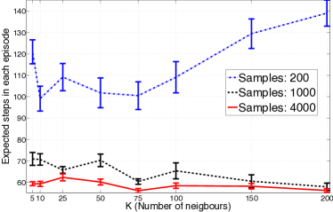
(a) Steps to goal

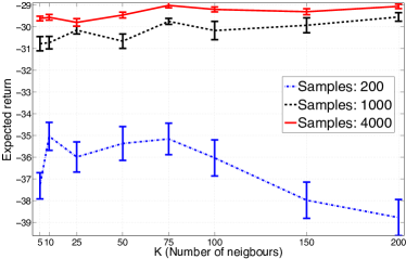
(b) Return

Figure 6: (Mountain-Car) The expected (a) number of steps to goal and (b) return in each episode as a function of $K$ in KNN-CAPI. The error bars show one standard error over 50 runs.

D-B Pole Balancing

(a) Number of steps

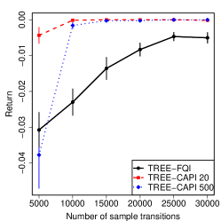
(b) Return

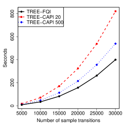
(c) Time

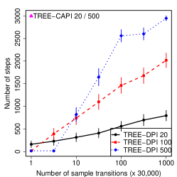
(d) Number of steps

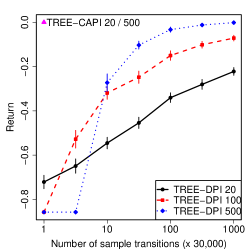
(e) Return

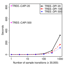
(f) Time

Figure 7: (Pole Balancing) Comparing the expected number of (a) number of steps, (b) return in each episode, and (c) computation time for Tree-based CAPI vs. Tree-based Fitted Q-Iteration as a function of sample size. Graphs (d), (e), and (f) compare Tree-based DPI (rollouts for PolicyEval) with Tree-based CAPI (Tree-FQI for PolicyEval). The error bars show one standard error over 50 runs.

We now turn to the pole-balancing problem, which is particularly interesting in the context of CAPI as it is possible to achieve good performance in this task with relatively simple policies [64].

For the pure value-based approach, we use Extra Trees Fitted Q-Iteration [21] (denoted by Tree-FQI), a state-of-the-art approximate value iteration algorithm, with the choice of 30 trees and the minimum number of points required to split a node as $\eta_{\mathrm{v}}=20$. We compare this value-based method with Tree-CAPI that uses the same Extra Tree Fitted Q-Iteration algorithm for policy evaluation (which is used, as before, only for policy evaluation, without improvement) and represents policies by an ensemble of $30$ trees. The Extra Trees algorithm was adopted to build the trees, but in this case using the estimated action-gap-weighted loss function. We chose the minimum number of points required to split a node from the set of $\eta_{\mathrm{\pi}}\in\{20,500\}$; note that this number controls the complexity of the policy space. We also compare performance with an instantiation of the DPI algorithm, which we call Tree-DPI. It uses rollouts for policy evaluation (as any DPI algorithm) and Extra Trees to represent the policy (with $\eta_{\mathrm{\pi}}\in\{20,100,500\})$. The rollouts are single trajectories of length at most $50$. We also run Tree-DPI for $5$ iterations. The number of trajectories are chosen such that Tree-DPI uses the same amount of data as Tree-CAPI. Hence the difference between Tree-DPI and Tree-CAPI is only in the policy evaluation step. In particular, Tree-DPI does not generalize the data using a value function, so it can only exploit policy regularities.

Figure 7 shows the expected number of steps balancing the pole (note that we stop the simulation after $3000$ successful steps). We also show the expected return per episode for all algorithms (averaged over $50$ independent runs) and the running time. Tree-CAPI clearly outperforms Tree-FQI (top row), especially when the number of samples is small and $\eta_{\mathrm{\pi}}$ is not very large. Note that for the sample sizes larger than $15000$, Tree-CAPI with any choice of $\eta_{\mathrm{\pi}}$ we tried solved the task perfectly, in all experiments. These results confirm that exploiting policy structure can lead to better and more stable results. The difference between the sample efficiency of both Tree-CAPI and Tree-FQI compared to Tree-DPI is dramatic: Tree-DPI-500 takes about $3\times 10^{7}$ samples to achieve the same performance that Tree-CAPI-20 achieved with about $10^{4}$ samples and Tree-FQI achieved with about $3\times 10^{4}$ samples. This comparison shows that value function regularities can also be exploited, especially when the number of samples is small. Note that Tree-CAPI is computationally more costly than Tree-DPI. In practice, the choice of algorithm depends on the cost of collecting new samples vs. the cost of computation. In problems when samples are expensive but computation can be done off-line, CAPI-style algorithms are a powerful choice, as illustrated in these results.

References

- Adams et al. [2004] B.M. Adams, H.T. Banks, Hee-Dae Kwon, and H.T. Tran. Dynamic multidrug therapies for HIV: optimal and STI control approaches. Mathematical Biosciences and Engineering, 1(2):223–41, 2004.
- Antos et al. [2008a] A. Antos, R. Munos, and Cs. Szepesvári. Fitted Q-iteration in continuous action-space MDPs. In Advances in Neural Information Processing Systems (NIPS), pages 9–16, 2008a.
- Antos et al. [2008b] A. Antos, Cs. Szepesvári, and R. Munos. Learning near-optimal policies with Bellman-residual minimization based fitted policy iteration and a single sample path. Machine Learning, 71:89–129, 2008b.
- Audibert and Tsybakov [2007] J.-Y. Audibert and A.B. Tsybakov. Fast learning rates for plug-in classifiers. The Annals of Statistics, 35(2):608–633, 2007.
- Bagnell et al. [2004] J. A. Bagnell, S. Kakade, A. Y. Ng, and J. Schneider. Policy search by dynamic programming. In Advances in Neural Information Processing Systems (NIPS). MIT Press, Cambridge, MA, 2004.
- Bartlett and Mendelson [2002] P. L. Bartlett and S. Mendelson. Rademacher and Gaussian complexities: Risk bounds and structural results. Journal of Machine Learning Research, 3:463–482, 2002.
- Bartlett et al. [2005] P. L. Bartlett, O. Bousquet, and S. Mendelson. Local Rademacher complexities. The Annals of Statistics, 33(4):1497–1537, 2005.
- Bartlett et al. [2006] P. L. Bartlett, M. I. Jordan, and J. D. McAuliffe. Convexity, classification, and risk bounds. Journal of the American Statistical Association, 101(473):138–156, 2006.
- Baxter and Bartlett [2001] J. Baxter and P.L. Bartlett. Infinite-horizon policy-gradient estimation. Journal of Artificial Intelligence Research, pages 319–350, 2001.
- Bertsekas [2005] D.P. Bertsekas. Dynamic programming and suboptimal control: A survey from ADP to MPC. European Journal of Control, 11(4-5):310–334, 2005.
- Bertsekas and Tsitsiklis [1996] D.P. Bertsekas and J.N. Tsitsiklis. Neuro-Dynamic Programming. Athena Scientific, 1996.
- Bhatnagar et al. [2009] S. Bhatnagar, R.S. Sutton, M. Ghavamzadeh, and M. Lee. Natural actor–critic algorithms. Automatica, 45(11):2471–2482, 2009.
- Bottou and Bousquet [2008] L. Bottou and O. Bousquet. The tradeoffs of large scale learning. In Advances in Neural Information Processing Systems (NIPS-20), pages 161–168, 2008.
- Boucheron et al. [2005] S. Boucheron, O. Bousquet, and G. Lugosi. Theory of classification: A survey of some recent advances. ESAIM: Probability and Statistics, 9:323–375, 2005.
- Buşoniu et al. [2010] L. Buşoniu, D. Ernst, B. De Schutter, and R. Babuska. Approximate dynamic programming with a fuzzy parameterization. Automatica, 46(5):804 – 814, 2010.
- Cao [2005] X.-R. Cao. A basic formula for online policy gradient algorithms. IEEE Trans. on Automatic Control, 50(5):696–699, 2005.
- Devroye et al. [1996] L. Devroye, L. Györfi, and G. Lugosi. A Probabilistic Theory of Pattern Recognition. Springer-Verlag New York, 1996.
- Dimitrakakis and Lagoudakis [2008] C. Dimitrakakis and M. G. Lagoudakis. Algorithms and bounds for rollout sampling approximate policy iteration. In European Workshop on Reinforcement Learning (EWRL), volume 5323 of Lecture Notes in Computer Science, pages 27–40. Springer, 2008.
- Dudley [1999] R. M. Dudley. Uniform Central Limit Theorems. Cambridge University Press, 1999.
- Engel et al. [2004] Y. Engel, S. Mannor, and R. Meir. The kernel recursive least-squares algorithm. IEEE Trans. on Signal Processing, 52(8):2275 – 2285, 2004.
- Ernst et al. [2005] D. Ernst, P. Geurts, and L. Wehenkel. Tree-based batch mode reinforcement learning. Journal of Machine Learning Research, 6:503–556, 2005.
- Ernst et al. [2006] D. Ernst, G.-B. Stan, J. Gongalves, and L. Wehenkel. Clinical data based optimal STI strategies for HIV: a reinforcement learning approach. In IEEE Conference on Decision and Control, pages 667–672, 2006.
- Farahmand [2011] A-m. Farahmand. Action-gap phenomenon in reinforcement learning. In Advances in Neural Information Processing Systems (NIPS), 2011.
- Farahmand and Precup [2012] A-m. Farahmand and D. Precup. Value pursuit iteration. In Advances in Neural Information Processing Systems (NIPS), 2012.
- Farahmand and Szepesvári [2011] A-m. Farahmand and Cs. Szepesvári. Model selection in reinforcement learning. Machine Learning Journal, 85(3):299–332, 2011.
- Farahmand et al. [2009a] A-m. Farahmand, M. Ghavamzadeh, Cs. Szepesvári, and S. Mannor. Regularized fitted Q-iteration for planning in continuous-space Markovian Decision Problems. In American Control Conference (ACC), pages 725–730, 2009a.
- Farahmand et al. [2009b] A-m. Farahmand, M. Ghavamzadeh, Cs. Szepesvári, and S. Mannor. Regularized policy iteration. In Advances in Neural Information Processing Systems (NIPS), pages 441–448, 2009b.
- Farahmand et al. [2010] A-m. Farahmand, R. Munos, and Cs. Szepesvári. Error propagation for approximate policy and value iteration. In Advances in Neural Information Processing Systems (NIPS), pages 568–576, 2010.
- Farahmand et al. [2012] A-m. Farahmand, D. Precup, and M. Ghavamzadeh. Generalized classification-based approximate policy iteration. In European Workshop on Reinforcement Learning (EWRL), 2012.
- Farahmand et al. [2013a] A-m. Farahmand, D. Precup, A.M.S Barreto, and M. Ghavamzadeh. CAPI: Generalized classification-based approximate policy iteration. In Multidisciplinary Conference on Reinforcement Learning and Decision Making, October 2013a.
- Farahmand et al. [2013b] A-m. Farahmand, D. Precup, M. Ghavamzadeh, and A.M.S Barreto. Classification-based approximate policy iteration. IEEE Trans. on Automatic Control (Submitted), 2013b.
- Fern et al. [2006] A. Fern, S. Yoon, and R. Givan. Approximate policy iteration with a policy language bias: Solving relational Markov Decision Processes. Journal of Artificial Intelligence Research, 25:85–118, 2006.
- Gabillon et al. [2011] V. Gabillon, A. Lazaric, M. Ghavamzadeh, and B. Scherrer. Classification-based policy iteration with a critic. In International Conference on Machine Learning (ICML), 2011.
- Geurts et al. [2006] P. Geurts, D. Ernst, and L. Wehenkel. Extremely randomized trees. Machine Learning, 36(1):3–42, 2006.
- Ghavamzadeh and Engel [2007] M. Ghavamzadeh and Y. Engel. Bayesian policy gradient algorithms. In Advances in Neural Information Processing Systems (NIPS), pages 457–464, 2007.
- Ghavamzadeh and Lazaric [2012] M. Ghavamzadeh and A. Lazaric. Conservative and greedy approaches to classification-based policy iteration. In Conference on Artificial Intelligence (AAAI), 2012.
- Ghavamzadeh et al. [2011] M. Ghavamzadeh, A. Lazaric, R. Munos, and M. Hoffman. Finite-sample analysis of Lasso-TD. In International Conference on Machine Learning (ICML), pages 1177–1184, 2011.
- Györfi et al. [2002] L. Györfi, M. Kohler, A. Krzyżak, and H. Walk. A Distribution-Free Theory of Nonparametric Regression. Springer Verlag, 2002.
- Kakade [2001] S. Kakade. A natural policy gradient. In Advances in Neural Information Processing Systems (NIPS), pages 1531–1538, 2001.
- Kakade and Langford [2002] S. Kakade and J. Langford. Approximately optimal approximate reinforcement learning. In International Conference on Machine Learning (ICML), pages 267–274, 2002.
- Kolter and Ng [2009] J. Z. Kolter and A. Y. Ng. Regularization and feature selection in least-squares temporal difference learning. In International Conference on Machine Learning (ICML), pages 521–528, 2009.
- Konda and Tsitsiklis [2001] V. R. Konda and J. N. Tsitsiklis. On actor-critic algorithms. SIAM Journal on Control and Optimization, pages 1143–1166, 2001.
- Lagoudakis and Parr [2003a] M.G. Lagoudakis and R. Parr. Least-squares policy iteration. Journal of Machine Learning Research, 4:1107–1149, 2003a.
- Lagoudakis and Parr [2003b] M.G. Lagoudakis and R. Parr. Reinforcement learning as classification: Leveraging modern classifiers. In International Conference on Machine Learning (ICML), pages 424–431, 2003b.
- Lazaric et al. [2010] A. Lazaric, M. Ghavamzadeh, and R. Munos. Analysis of a classification-based policy iteration algorithm. In International Conference on Machine Learning (ICML), pages 607–614, 2010.
- Lazaric et al. [2012] A. Lazaric, M. Ghavamzadeh, and R. Munos. Finite-sample analysis of least-squares policy iteration. Journal of Machine Learning Research, pages 3041–3074, 2012.
- Li et al. [2007] L. Li, V. Bulitko, and R. Greiner. Focus of attention in reinforcement learning. Journal of Universal Computer Science, 13(9):1246–1269, 2007.
- Marbach and Tsitsiklis [2001] P. Marbach and J.N. Tsitsiklis. Simulation-based optimization of Markov reward processes. IEEE Trans. on Automatic Control, 46(2):191–209, 2001.
- Munos [2003] R. Munos. Error bounds for approximate policy iteration. In International Conference on Machine Learning (ICML), pages 560–567, 2003.
- Munos [2007] R. Munos. Performance bounds in norm for approximate value iteration. SIAM Journal on Control and Optimization, pages 541–561, 2007.
- Peters et al. [2003] J. Peters, Vijayakumar S., and S. Schaal. Reinforcement learning for humanoid robotics. In IEEE-RAS International Conference on Humanoid Robots, 2003.
- Riedmiller [2005] M. Riedmiller. Neural fitted Q iteration – first experiences with a data efficient neural reinforcement learning method. In European Conference on Machine Learning, pages 317–328, 2005.
- Ross et al. [2011] S. Ross, G. Gordon, and J. A. Bagnell. A reduction of imitation learning and structured prediction to no-regret online learning. In Artifical Intelligence and Statistics (AISTATS), April 2011.
- Scherrer and Lesner [2012] B. Scherrer and B. Lesner. On the use of non-stationary policies for stationary infinite-horizon markov decision processes. In Advances in Neural Information Processing Systems (NIPS), pages 1835–1843. 2012.
- Scherrer et al. [2012] B. Scherrer, M. Ghavamzadeh, V. Gabillon, and M. Geist. Approximate modified policy iteration. In International Conference on Machine Learning (ICML), 2012.
- Steinwart and Christmann [2008] I. Steinwart and A. Christmann. Support Vector Machines. Springer, 2008.
- Sutton et al. [2009] R. S. Sutton, H. R. Maei, D. Precup, S. Bhatnagar, D. Silver, Cs. Szepesvári, and E. Wiewiora. Fast gradient-descent methods for temporal-difference learning with linear function approximation. In International Conference on Machine Learning (ICML), pages 993–1000. ACM, 2009.
- Sutton and Barto [1998] R.S. Sutton and A.G. Barto. Reinforcement Learning: An Introduction. The MIT Press, 1998.
- Szepesvári [2010] Cs. Szepesvári. Algorithms for Reinforcement Learning. Morgan Claypool Publishers, 2010.
- Taylor and Parr [2009] G. Taylor and R. Parr. Kernelized value function approximation for reinforcement learning. In International Conference on Machine Learning (ICML), pages 1017–1024, 2009.
- Tesauro and Galperin [1996] G. Tesauro and G.R. Galperin. On-line policy improvement using Monte-Carlo search. In Advances in Neural Information Processing Systems (NIPS), 1996.
- Tsitsiklis and Van Roy [1997] J. N. Tsitsiklis and B. Van Roy. An analysis of temporal difference learning with function approximation. IEEE Trans. on Automatic Control, 42:674–690, 1997.
- Wasserman [2007] L. Wasserman. All of Nonparametric Statistics. Springer, 2007.
- Wieland [1991] A. P. Wieland. Evolving neural network controllers for unstable systems. In International Joint Conference on Neural Networks (IJCNN), pages 667–673, 1991.