Calibrated Langevin dynamics simulations of intrinsically disordered proteins

Abstract

We perform extensive coarse-grained (CG) Langevin dynamics simulations of intrinsically disordered proteins (IDPs), which possess fluctuating conformational statistics between that for excluded volume random walks and collapsed globules. Our CG model includes repulsive steric, attractive hydrophobic, and electrostatic interactions between residues and is calibrated to a large collection of single-molecule fluorescence resonance energy transfer data on the inter-residue separations for $36$ pairs of residues in five IDPs: $\alpha$-, $\beta$-, and $\gamma$-synuclein, the microtubule-associated protein $\tau$, and prothymosin $\alpha$. We find that our CG model is able to recapitulate the average inter-residue separations regardless of the choice of the hydrophobicity scale, which shows that our calibrated model can robustly capture the conformational dynamics of IDPs. We then employ our model to study the scaling of the radius of gyration with chemical distance in $11$ known IDPs. We identify a strong correlation between the distance to the dividing line between folded proteins and IDPs in the mean charge and hydrophobicity space and the scaling exponent of the radius of gyration with chemical distance along the protein.

1 Introduction

Intrinsically disordered proteins (IDPs) do not possess well-defined three-dimensional structures as globular proteins do. Instead, they display highly fluctuating conformational dynamics with little or no persistent secondary structure in physiological conditions [49]. IDPs are more expanded than collapsed globules, but more compact than self-avoiding random coils [39]. Because IDPs are structurally disordered and sample many different conformations, they can interact and bind to a wide variety of targets and participate in many important cellular processes [11]. A number of studies have also shown that IDPs can aggregate to form oligomers and fibrils that are rich in $\beta$-sheet secondary structure and linked to the development of amyloid diseases such as Parkinson’s and Alzheimer’s disease [8, 18].

There has been a significant research effort aimed at experimentally measuring and modeling the conformational dynamics of single IDPs. Although x-ray crystallography has provided the positions of each atom (accurate in many cases to $<1$Å) in thousands of folded proteins, static representations of the atomic positions in IDPs cannot be obtained from x-ray crystallography, and such representations are not even meaningful for IDPs [10]. Alternatively, many groups have employed single-molecule fluorescence resonance energy transfer (smFRET) to obtain the separation distributions between specific pairs of residues for IDPs in solution. In brief, smFRET involves exciting a donor fluorophore with a laser, which then selectively excites an acceptor fluorophore depending on the distance between the two labeled residues. The donor or acceptor excitation then decays, emitting a photon. The donor and acceptor emit two different wavelengths of light, and the ratio of the two emitted wavelengths gives the average distance between the two residues. To date, smFRET has been performed on tens of IDPs, but data for the distribution of inter-residue separations has been obtained only for several pairs of residues for each protein. In addition, small-angle x-ray scattering (SAXS) [46, 48, 24, 41, 34, 15], nuclear magnetic resonance (NMR) [7, 35], and fluorescence correlation spectroscopy (FCS) [29, 32] have been performed on a number of IDPs. These provide more coarse measurements of the structure of the protein, such as the radius of gyration (or hydrodynamic radius), which characterizes the average size of the protein.

In a recent manuscript [38], we introduced a physical model to describe the fluctuating conformational dynamics of IDPs. The motivation for the new computational model for IDPs stems in part from the fact that commonly used molecular mechanics force fields, such as Amber [36] and CHARMM [3], can bias the simulation results toward folded behavior since they have been calibrated using x-ray crystal structures of folded proteins [26]. Our physical model includes repulsive steric interactions, screened electrostatic interactions between charged residues, and attractive hydrophobic interactions between $C_{\alpha}$ atoms. We employed two representations of IDPs at different spatial scales. The united-atom (UA) description provides a realistic atomic-level representation of protein stereochemistry, whereas the coarse-grained (CG) description employs one bead per residue with bond-length, bond-angle, and backbone dihedral-angle potentials derived from interactions in the UA description.

For both UA and CG descriptions, the model requires only one free parameter that gives the ratio of the hydrophobic to electrostatic energy scales. In our previous work [38], we determined this ratio by matching Langevin dynamics simulations of the model to experimental smFRET data for the inter-residue separations for the IDP, $\alpha$-synuclein. We then showed that our calibrated Langevin dynamics simulations for $\alpha$-synuclein were able to accurately recapitulate SAXS measurements of the radius of gyration and give conformational statistics that are intermediate between random walk and collapsed globule behavior. An advantage of our calibrated Langevin dynamics simulations over constraint methods is that they do not assume random walk statistics with artificial constraints imposed on the inter-residue separation distributions [31].

In this manuscript, we present extensive new results on the CG description of IDPs. We improve the calibration of the CG model by considering a larger dataset of smFRET results from experiments that includes five IDPs: $\alpha$-, $\beta$-, and $\gamma$-synuclein ($\alpha$S, $\beta$S, and $\gamma$S), the microtubule-associated protein $\tau$ (MAPT), and prothymosin $\alpha$ (ProT$\alpha$). For this set of proteins, there is smFRET data on a total of $36$ pairs of residues ($\alpha$S: $12$ [43, 42]; $\beta$S and $\gamma$S: $5$ each [9]; MAPT: $12$ [31]; and ProT$\alpha$: $2$ [19]), which includes most of the smFRET data that is currently available for IDPs. In future work, our CG Langevin dynamics simulations can be employed to study association, aggregation, and formation of $\beta$-strand order in systems containing multiple IDPs.

IDPs typically possess low mean hydrophobicity and high mean charge relative to folded proteins, with a dividing line in charge-hydrophobicity space that separates the two [45, 25]. The synucleins and MAPT are both close to the dividing line, whereas ProT$\alpha$ is highly charged with relatively low hydrophobicity, and is in this sense an ideal IDP. What physical properties distinguish IDPs that are close versus far from the folded protein/IDP dividing line? In this study, we perform calibrated Langevin dynamics simulations of CG descriptions of IDPs to investigate the effects of hydrophobicity and charge on the conformational statistics of IDPs. A significant result of our work is that we find a strong correlation between the distance to the folded protein/IDP dividing line and the scaling exponent of the radius of gyration with chemical distance along the protein.

Our manuscript is organized as follows. In Sec. 2, we describe Langevin dynamics simulations of the CG model for IDPs and discuss important biological and physical aspects of the IDPs we consider. In Sec. 3, we demonstrate that the calibrated Langevin dynamics accurately recapitulate the available smFRET and SAXS experimental data and that the results are robust to variations in how we model hydrophobicity. We then describe our studies of the scaling of the radius of gyration with chemical distance for a large sample of known IDPs. Finally, in Sec. 4, we discuss the implications of our results on future research of IDPs.

2 Methods

Amino acid type	$\alpha$S	$\beta$S	$\gamma$S	MAPT	ProT$\alpha$
ALA	$19$	$18$	$16$	$34$	$11$
ARG${}^{\text{+}}$	$0$	$2$	$2$	$14$	$2$
ASN	$3$	$1$	$4$	$11$	$6$
ASP${}^{\text{-}}$${}^{\text{r}}$	$6$	$3$	$3$	$29$	$19$
CYS	$0$	$0$	$0$	$2$	$0$
GLN	$6$	$6$	$6$	$19$	$2$
GLU${}^{\text{-}}$	$18$	$25$	$20$	$27$	$34$
GLY	$18$	$13$	$10$	$49$	$9$
HIS${}^{\text{+}}$	$1$	$1$	$0$	$12$	$0$
ILE${}^{\text{a}}$	$2$	$2$	$2$	$15$	$1$
LEU${}^{\text{a}}$	$4$	$7$	$1$	$21$	$1$
LYS${}^{\text{+}}$	$15$	$11$	$15$	$44$	$8$
MET	$4$	$4$	$2$	$6$	$1$
PHE${}^{\text{a}}$	$2$	$3$	$2$	$3$	$0$
PRO${}^{\text{r}}$	$5$	$8$	$2$	$43$	$1$
SER	$4$	$6$	$10$	$45$	$4$
THR	$10$	$7$	$10$	$35$	$6$
TRP${}^{\text{a}}$	$0$	$0$	$0$	$0$	$0$
TYR	$4$	$4$	$1$	$5$	$0$
VAL	$19$	$13$	$21$	$27$	$5$
Total	$140$	$134$	$127$	$441$	$110$

Table 1: Numbers of each amino acid type in $\alpha$S, $\beta$S, $\gamma$S, MAPT, and ProT$\alpha$. ‘+’ and ‘-’ denote positively and negatively charged residues, respectively (Table 3). ‘a’ and ‘r’ indicate highly hydrophobic ($\epsilon_{i}\sim 1$) and hydrophilic ($\epsilon_{i}\sim 0$) residues using the scaled and shifted Monera hydrophobicity scale described in Sec. 2.

This manuscript focuses on the conformational dynamics of IDPs, including the synuclein family ($\alpha$S, $\beta$S, and $\gamma$S), MAPT, and ProT$\alpha$. Table 1 provides the numbers of each amino acid type in these five IDPs. In Fig. 1, we show the hydrophobicity and electric charge averaged over nearby residues as a function of the residue index (originating at the N-terminus) for each IDP and the folded protein lysozyme C [13, 4].

The synucleins are a family of small proteins commonly expressed in neuronal tissue [18]. They possess hydrophilic and negatively charged C-terminal regions [44, 20, 21]. MAPT is a microtubule-associated protein commonly expressed in neurons [17]. We study isoform F of MAPT with $441$ residues [16]. The N-terminus is negatively charged, while the remainder is nearly neutral, and most of the protein is slightly hydrophilic. ProT$\alpha$, with $110$ residues, is both highly charged and hydrophilic [14, 30]. Note that the net hydrophobicity is larger and the net charge is much smaller for the folded protein lysozyme C compared to the IDPs.

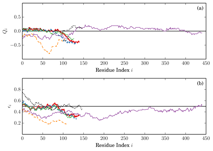
Figure 1: (Color online) (a) Electric charge $Q_{i}$ (in units of the electron charge $q_{e}$) and (b) hydrophobicity $\epsilon_{i}$ as a function of the residue index $i$ originating from the N-terminus for the IDPs $\alpha$S (thick, solid red line), $\beta$S (thick, dashed blue line), $\gamma$S (thick, dotted green line), MAPT (thin, solid purple line), ProT$\alpha$ (thin, dashed orange line) and the folded protein lysozyme C (thin, dotted black line). We quote the normalized and shifted Monera hydrophobicity scale [28], where $0$ is the least and $1$ is the most hydrophobic. (See Eq. 7.) Data for each $i$ is averaged over $31$ nearby residues, with data at the endpoints reflected beyond the endpoints to reduce edge effects.

Coarse-grained model

We model IDPs using a coarse-grained description [5] of the backbone of a protein chain, where each residue $i$ is represented by a spherical bead with diameter $\sigma$, mass $M_{i}$, hydrophobicity $\epsilon_{i}$, and charge $Q_{i}$. The bond lengths and bond angles are constrained using linear spring potentials:

$$V^{bl}=\frac{k_{\ell}}{2}\sum_{\left\langle ij\right\rangle}\left(r_{ij}-\ell\right)^{2}$$ (1)

$$V^{ba}=\frac{k_{\theta}}{2}\sum_{\left\langle ijk\right\rangle}\left(\theta_{ijk}-\theta_{0}\right)^{2},$$ (2)

where $\langle ij\rangle$ ($\langle ijk\rangle$) indicates a sum over distinct pairs (triples) of adjacent beads, $r_{ij}$ is the separation between the centers of beads $i$ and $j$, and $\theta_{ijk}$ is the angle between the bonded residues $i$, $j$, and $k$. The average bond length $\langle r_{ij}\rangle=\ell$, bond angle $\langle\theta_{ijk}\rangle=\theta_{0}$, and the spring constants $k_{l}$ and $k_{\theta}$ in Eqs. 1 and 2 are obtained by calculating the average and standard deviation of $r_{ij}$ and $\theta_{ijk}$ from Langevin dynamics of the UA model for the five IDPs we considered with hard-sphere atomic interactions and stereochemical constraints obtained from the Dunbrack database of high-resolution protein crystal structures [50]. We found $\ell=$3.9\text{\,}\mathrm{\SIUnitSymbolAngstrom}$$, $(k_{\ell}/k_{b}T)^{-\frac{1}{2}}=$0.046\text{\,}\mathrm{\SIUnitSymbolAngstrom}$$, $\theta_{0}=$2.12\text{\,}\mathrm{r}\mathrm{a}\mathrm{d}\mathrm{i}\mathrm{a}\mathrm{n}\mathrm{s}$$, and $(k_{\theta}/k_{b}T)^{-\frac{1}{2}}=$0.26\text{\,}\mathrm{r}\mathrm{a}\mathrm{d}\mathrm{i}\mathrm{a}\mathrm{n}\mathrm{s}$$ for simulations of $\alpha$S, where $T$ is the temperature. Similar results are found for the other four IDPs.

$n$	$A_{n}$	$B_{n}$
$1$	$0.705$	$-0.175$
$2$	$-0.313$	$-0.093$
$3$	$-0.079$	$0.030$
$4$	$0.041$	$0.030$

Table 2: The four Fourier coefficients of the backbone dihedral angle potential $V^{da}$ in Eq. 3 that are employed to recapitulate the probability distribution $P^{UA}(\phi_{ijkl})$ of backbone dihedral angles (defined by four consecutive C_α atoms) from UA simulations of $\alpha$S.

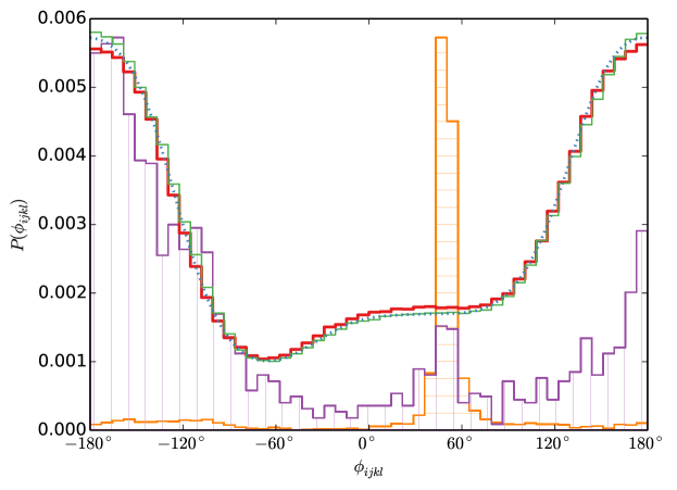
Figure 2: (Color online) The backbone dihedral angle distribution $P^{UA}(\phi_{ijkl})$ obtained from the UA description of $\alpha$S (light green solid line) with only hard-sphere atomic interactions plus stereochemical constraints obtained from the Dunbrack database of high-resolution protein crystal structures. We fit $P^{UA}(\phi_{ijkl})$ for the UA model using four coefficients (Table 2) in the Fourier series in Eq. 3 (blue dotted line). We show that $P^{CG}(\phi_{ijkl})$ from Langevin dynamics simulations of the CG model for $\alpha$S with only bond-length, bond-angle, and dihedral angle interactions in Eqs. 1, 2, and 3 (thick solid red line) matches that from the hard-sphere UA model for $\alpha$-synuclein. $P(\phi_{ijkl})$ from stretches of $\alpha$-helices (orange horizontal lines) and $\beta$-sheets (purple vertical lines) that are longer than $10$ residues in the Dunbrack database of high-resolution protein crystal structures are also shown for comparison. For ease of visual comparison, the dihedral angle distributions from $\alpha$-helical and $\beta$-sheet structures were not normalized.

We show the probability distribution $P^{UA}(\phi_{ijkl})$ of backbone dihedral angles (defined for four consecutive C_α atoms) from Langevin dynamics simulations of the UA model for $\alpha$S with hard-sphere atomic interactions and stereochemical constraints on the bond-lengths and angles in Fig. 2. (Similar results are found for the other four IDPs.) The distribution possesses a large broad peak at $\phi_{ijkl}=\pm 180^{\circ}$ and a plateau in the range $0^{\circ}<\phi_{ijkl}<120^{\circ}$. The broad peak and plateau region in $P^{UA}(\phi_{ijkl})$ arise from the $\beta$-sheet and $\alpha$-helix backbone conformations, respectively. We assume that a fourth-order Fourier series can describe an effective backbone dihedral angle potential,

$$V^{da}=\sum_{\left\langle ijkl\right\rangle}\sum_{n=1}^{4}A_{n}\cos\left(n\phi_{ijkl}\right)+B_{n}\sin\left(n\phi_{ijkl}\right),$$ (3)

that governs $P^{CG}(\phi_{ijkl})$ for the CG model. In Eq. 3, $\langle ijkl\rangle$ indicates all distinct combinations of four bonded residues ($i$, $j$, $k$, and $l$) along the chain and the coefficients $A_{n}$ and $B_{n}$ are obtained by inverting the probability distribution $P^{UA}(\phi_{ijkl})=P^{CG}(\phi_{ijkl})$. $V^{da}=-k_{b}T\langle\ln P^{CG}(\phi_{ijkl})\rangle$ with the coefficients $A_{n}$ and $B_{n}$ given in Table 2.

As in our previous studies [38], we employed a purely repulsive Weeks-Chandler-Andersen (WCA) potential, the attractive part of the Lennard-Jones potential, and screened Coulomb potential to model the steric, hydrophobic, and electrostatic interactions, respectively:

$$V^{r}=\epsilon_{r}\sum_{ij}\left(4\left[\left(\frac{\sigma}{r_{ij}}\right)^{12}-\left(\frac{\sigma}{r_{ij}}\right)^{6}\right]+1\right)\\ \Theta\left(2^{\frac{1}{6}}\sigma-r_{ij}\right)$$ (4)

$$V^{a}=\epsilon_{a}\sum_{ij}\left[\epsilon_{ij}\left(4\left[\left(\frac{\sigma}{r_{ij}}\right)^{12}-\left(\frac{\sigma}{r_{ij}}\right)^{6}\right]+1\right)\right.\\ \left.\times\Theta\left(r_{ij}-2^{\frac{1}{6}}\sigma\right)-\epsilon_{ij}\right]$$ (5)

$$V^{es}= \epsilon_{es}\sum_{ij}\frac{Q_{i}Q_{j}}{q_{e}^{2}}\frac{\sigma}{r_{ij}}e^{-\frac{r_{ij}}{\lambda}},$$ (6)

where $\Theta(x)$ is the Heaviside step function, $\sigma=$4.8\text{\,}\mathrm{\SIUnitSymbolAngstrom}$$ is the average distance between the centers of mass of neighboring residues, and $Q_{i}$ is the electric charge associated with each of the charged residues LYS, ARG, HIS, ASP, and GLU (Table 3). The WCA potential $V^{r}$ is zero for $r_{ij}>2^{1/6}\sigma$, the hydrophobicity potential $V^{a}$ includes a $-1/r^{6}_{ij}$ attractive tail, and the screened Coulomb potential $V^{es}$ is negligible beyond the screening length $\lambda$. The mixing rule $\epsilon_{ij}$ for the (shifted and normalized) hydrophobicity index $0\leq\epsilon_{i}\leq 1$ for each residue $i$ will be discussed in Sec. 2. ${\overline{\epsilon}_{es}}=\epsilon_{es}/k_{b}T$ is a parameter that controls the strength of the electrostatic interactions. Typical experimental solution conditions with $150$ mM salt concentration, $p\text{H}=7.4$, and temperature $T=293$ K yield $\lambda=$9\text{\,}\mathrm{\SIUnitSymbolAngstrom}$$ and ${\overline{\epsilon}}_{es}=\kappa_{es}=q_{e}^{2}/(4\pi\epsilon_{0}D\sigma k_{b}T)\approx 1.485$, where $D=80$ is the permittivity of water. For most of the simulations, we set the energy scale for the repulsive interactions $\epsilon_{r}/k_{b}T=1$ and calibrate the ratio of strength of the hydrophobic interactions to that of the electrostatic interactions $\alpha_{CG}={\overline{\epsilon}}_{a}/\kappa_{es}$ to match the smFRET data.

Residue	Residue charge $Q_{i}$
LYS	$1$
ARG	$1$
HIS	$0.1$
ASP	$-1$
GLU	$-1$

Table 3: Electric charge $Q_{i}$ (in units of the electron charge $q_{e}$) for the charged residues LYS, ARG, HIS, ASP, and GLU [33].

Hydrophobicity models

We model hydrophobic interactions between residues using the attractive part of the Lennard-Jones potential (Eq. 5). In this section, we describe the possible choices for assigning the hydrophobicity index $\epsilon_{i}$ to each residue and mixing rule $\epsilon_{ij}$ for pairwise hydrophobic interactions between residues $i$ and $j$.

There are many different hydrophobicity scales for assigning the hydrophobicity for whole residues [6], and each scale has its own mean, maximum, and minimum. To enable comparison between different hydrophobicity scales, we shifted and normalized the original values ${\widetilde{\epsilon}}_{i}$ to obtain

$$\epsilon_{i}=\frac{{\widetilde{\epsilon}}_{i}-\min_{i}({\widetilde{\epsilon}}_{i})}{\max_{i}({\widetilde{\epsilon}}_{i})-\min_{i}({\widetilde{\epsilon}}_{i})}$$ (7)

with $0\leq\epsilon_{i}\leq 1$ as shown in Fig. 3.

Below, we investigate the sensitivity of the simulation results to three choices for the hydrophobicity scales: 1) the shifted and normalized Kyte-Doolittle [23] scale, 2) the shifted and normalized Monera [28] scale, and 3) an average of seven commonly used hydrophobicity scales (Kyte-Doolittle, Monera, augmented Wimley-White [51, 52], Eisenberg [12], Miyazawa [27], Sharp  [37], and Sharp (corrected for solvent-solute size differences [37])). The “average” scale is obtained by averaging the seven shifted and normalized scales, and then shifting and normalizing the result.

We also consider the sensitivity of the simulation results to three pairwise mixing rules for the shifted and normalized hydrophobicities $\epsilon_{i}$ and $\epsilon_{j}$: 1) arithmetic mean: $\epsilon_{ij}=(\epsilon_{i}+\epsilon_{j})/2$, 2) geometric mean: $\epsilon_{ij}=\sqrt{\epsilon_{i}\epsilon_{j}}$, and 3) maximum: $\epsilon_{ij}=\max(\epsilon_{i},\epsilon_{j})$. Below, we will show results (Sec. 3) for Langevin dynamics simulations of the five IDPs ($\alpha$S, $\beta$S, and $\gamma$S, MAPT, and ProT$\alpha$) using nine different models for the pairwise hydrophobic interactions between residues ($3$ hydrophobicity scales, each with $3$ mixing rules).

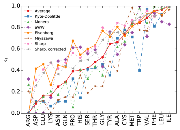
Figure 3: (Color online) Seven commonly used hydrophobicity scales (Kyte-Doolittle [23], Monera [28], Wimley-White [51, 52], Eisenberg [12], Miyazawa [27], Sharp, and Sharp with solvent-solute size difference corrections [37]) for each amino acid type that have been shifted and normalized so that $0\leq\epsilon_{i}\leq 1$. The “average” value for each residue indicates the shifted and normalized average over the seven shifted and normalized hydrophobicity scales. The residues are ordered according to their average $\epsilon_{i}$.

Langevin dynamics simulations

We performed coarse-grained Langevin dynamics simulations of single IDPs at fixed temperature $T=$293\text{\,}\mathrm{K}$$ with bond-length, bond-angle, dihedral-angle, steric, hydrophobic, and screened Coulomb interactions (Eqs. 1–6). We employed free boundary conditions, a modified velocity-Verlet integration scheme with a Langevin thermostat [2], damping coefficient $\gamma=0.001\sqrt{\frac{k_{B}T}{m_{0}\ell_{0}^{2}}}\approx$16\text{\,}{\mathrm{ns}}^{-1}$$, and fixed time step $\Delta t=0.03\sqrt{\frac{m_{0}\ell_{0}^{2}}{k_{B}T}}\approx$1.9\text{\,}\mathrm{fs}$$, where $m_{0}=1{\rm Da}$ and $\ell_{0}=$1\text{\,}\mathrm{\SIUnitSymbolAngstrom}$$. We chose the time step $\Delta t$ so that the relative energy fluctuations in the absence of the thermostat satisfy $\frac{\sqrt{\left<E^{2}\right>-\left<E\right>^{2}}}{\left<E\right>}<$1\text{\times}{10}^{-4}$$ and the damping parameter so that $1/\gamma$ is much smaller than total run time $t_{\rm tot}=$0.5\text{\,}\mathrm{\SIUnitSymbolMicro s}$$. The chains were initialized in a zig-zag conformation with random velocities at temperature $T$ and then equilibrated for $10^{4}t_{R}$, where $t_{R}$ is the time for the normalized $R_{g}$ autocorrelation function to decay to $1/e$. After equilibration, production runs were conducted to measure the inter-residue separations and radius of gyration for each IDP.

3 Results

smFRET efficiencies

In Fig. 4, we show experimental results for the smFRET efficiencies for $12$ inter-residue separations for $\alpha$S [43, 42], $5$ for $\beta$S and $\gamma$S [9], $2$ for ProT$\alpha$ [19], and $12$ for MAPT [31]. Large $ET_{\rm eff}$ indicate small average inter-residue separations and vice versa. The smFRET efficiencies depend strongly on the separation $r_{ij}$ between residue pairs,

$$ET_{\text{eff}}=\left\langle\frac{1}{1+\left(\frac{r_{ij}}{R_{0}}\right)^{6}}\right\rangle$$ (8)

where $R_{0}=$54\text{\,}\mathrm{\SIUnitSymbolAngstrom}$$ is the Förster distance for the donor-acceptor pair (Alexa Fluor 488–Alexa Fluor 594), angle brackets indicate a time average, and we assume that the finite size of the fluorophores has a negligible effect on $ET_{\rm eff}$. We directly measure $ET_{\rm eff}$ for each IDP in our simulations, and compare it to the experimental values. For most simulations, we varied the ratio of the hydrophobic to the electrostatic interactions $\alpha_{CG}$ (i.e. change ${\overline{\epsilon}}_{a}$ at fixed ${\overline{\epsilon}}_{es}=\kappa_{es}$) to minimize the root-mean-square deviation in $ET_{\rm eff}$ between the simulations and experiments:

$$\Delta=\sqrt{\frac{1}{N_{p}}\sum_{i=1}^{N_{p}}(ET^{\rm exp}_{\rm eff}(i)-ET^{\rm sim}_{\rm eff}(i))^{2}},$$ (9)

where $ET^{\rm exp}_{\rm eff}(i)$ is the FRET efficiency for residue pair $i$ from experiments and $N_{p}$ is the number of residue pairs. For the simulations described in this section, we employ the shifted and normalized Monera hydrophobicity scale with the geometric mean as the mixing rule.

For $\alpha$S, the experimental values for $ET_{\rm eff}$ for the $12$ residue pairs vary from $\approx 0.90$ to $0.40$ as shown in Fig. 4. From the CG Langevin dynamics simulations of $\alpha$S, we find that $\alpha_{CG}\approx$0.48\pm 0.03$$ minimizes the root-mean-square deviation between the simulations and experiments. This optimized value of $\alpha_{CG}$ yields $\Delta_{\rm min}\approx$0.06\pm 0.02$$ (Fig. 6), which indicates close agreement between simulations and experiments. (The error bar for $\alpha_{CG}$ was obtained by determining the change in $\alpha_{CG}$ necessary for $\Delta$ to increase beyond the error bars of $\Delta_{\rm min}$.) In contrast, when the strength of the hydrophobic interactions is set to zero ($\alpha_{CG}=0$), $ET_{\rm eff}$ for the simulations are significantly below the experimental values for all residue pairs with $\Delta\approx$0.26$$. To investigate the relative contributions of the hydrophobic and electrostatic interactions to $ET_{\rm eff}$, we also performed simulations with ${\overline{\epsilon}}_{es}=0$ and $\alpha_{CG}=0.48$. We find that the quality of the match between simulations and experiments is comparable for the simulations with ($\Delta\approx$0.06\pm 0.02$$) and without ($\Delta\approx$0.08\pm 0.02$$) electrostatic interactions.

We find that $\alpha_{CG}\approx$0.48\pm 0.03$$ yields the best match of the FRET efficiencies from the CG simulations and experiments for $\alpha$S. This value of the ratio of the hydrophobic and electrostatic interactions differs by about a factor of 2.5 from the optimal value ($\alpha_{UA}\approx 1.2$) obtained from our previous UA simulations of $\alpha$S [38]. This result shows that the optimal numerical value of $\alpha$ can be sensitive to the geometrical representation of residues in IDPs, as well as the hydrophobicity scale implemented in the model.

For $\beta$S and $\gamma$S, the FRET efficiencies for three of the five residue pairs (with similar chemical distances) are approximately equal ($ET_{\rm eff}\approx 0.85$), while $ET_{\rm eff}$ for the other two pairs drop to $0.6$ and $0.2$ (Fig. 4). Similar to the results for $\alpha$S, the root-mean-square deviation in $ET_{\rm eff}$ between simulations and experiments is minimized when $\alpha_{CG}\approx$0.42\pm 0.07$$ and $0.46\pm 0.05$ for $\beta$S ($\Delta_{\rm min}\approx 0.02$) and $\gamma$S ($\Delta_{\rm min}\approx 0.04$) respectively (Fig. 6). In addition, the CG simulations with ${\overline{\epsilon}}_{es}=0$ and $\alpha_{CG}=0.42$ ($0.46$) show reasonable agreement with the experimental $ET_{\rm eff}$ for $\beta$S ($\gamma$S) with $\Delta\approx 0.10$ ($0.04$), except for residue pair 102–126 for $\beta$S. For ProT$\alpha$ (Fig. 4), we find that $\Delta$ is minimized for $\alpha_{CG}\approx$0.64\pm 0.36$$. The optimal $\alpha_{CG}$ for ProT$\alpha$ has larger error bars because $\Delta(\alpha_{CG})$ is nearly flat. These error bars encompass the optimal $\alpha_{CG}$ for $\alpha$S, $\beta$S, and $\gamma$S.

The $ET_{\rm eff}$ for MAPT is more complex. In Fig. 5, we show $ET_{\rm eff}$ for MAPT for residue pairs ordered from small to large chemical distances along the protein chain. Despite the monotonic increase in chemical distance from left to right, $ET_{\rm eff}$ shows an anomalously large drop for residue pair 103–183 followed by an increase in $ET_{\rm eff}$ even though the chemical distance continues to increase. This behavior differs from the dependence of $ET_{\rm eff}$ on chemical distance for the synuclein family and ProT$\alpha$, where $ET_{\rm eff}$ decreases roughly monotonically with chemical distance with only minor fluctuations. In Fig. 6, we show that $\Delta$ is minimized at $\alpha_{CG}\approx$0.52\pm 0.02$$. This yields $\Delta_{\min}\approx$0.09\pm 0.02$$, which is significantly larger than that for the other IDPs (0.02, 0.02, 0.04, and 0.06). In particular, the CG model with the optimal $\alpha_{CG}$ shows large deviations with the experimental $ET_{\rm eff}$ for residue pairs 354–433, 103–184, and 17–103. Although the CG model without electrostatic interactions (${\overline{\epsilon}}_{es}=0$ and $\alpha_{CG}=0.52$) is able to recapitulate $ET_{\rm eff}$ for the synuclein family and ProT$\alpha$, it yields $\Delta_{\rm min}\approx 0.18$ for MAPT. In the electrostatics-only CG model, we find that $\Delta_{\rm min}\approx 0.34$, which is much larger than $\Delta_{\rm min}$ for the CG model with both hydrophobic and electrostatic interactions.

We find that for the synucleins and ProT$\alpha$, optimized models with and without electrostatics interactions provide an accurate description of the experimental $ET_{\rm eff}$. However, the optimized model with both electrostatic and hydrophobic interactions provides the best match to experimental $ET_{\rm eff}$ for MAPT. More importantly, the minimal RMS deviations in $ET_{\rm eff}$ between simulations and experiment for MAPT are larger than those for the synuclein family and ProT$\alpha$ as well as typical experimental error bars. The fact that MAPT is three times as long as, and less charged and hydrophobic (Fig. 8) than the other IDPs may contribute to the larger RMS deviations [40].

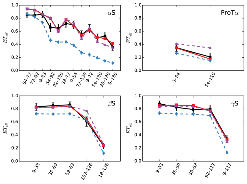
Figure 4: (Color online) FRET efficiencies $ET_{\rm eff}$ for $\alpha$S (upper left), ProT$\alpha$ (upper right), $\beta$S (lower left), and $\gamma$S (lower right) from experimental measurements (black circles) and CG Langevin dynamics simulations. We include data for three choices for the strength of the hydrophobic and electrostatic interactions ${\overline{\epsilon}}_{a}$ and ${\overline{\epsilon}}_{es}$ for each IDP: 1) ${\overline{\epsilon}}_{a}=0$ and ${\overline{\epsilon}}_{es}=\kappa_{es}$ such that the chains behave as extended coils (blue diamonds), 2) the optimal $\alpha_{CG}$ for each protein with ${\overline{\epsilon}}_{es}=\kappa_{es}$, where the root-mean-square deviations between the experimental and simulation $ET_{\rm eff}$ are minimized (red squares), and 3) the optimal $\alpha_{CG}$ for each protein with no electrostatic interactions ${\overline{\epsilon}}_{es}=0$ (purple triangles). The error bars for $ET_{\rm eff}$ from the simulations give the error in the mean. Error bars that are not visible are smaller than the symbols.

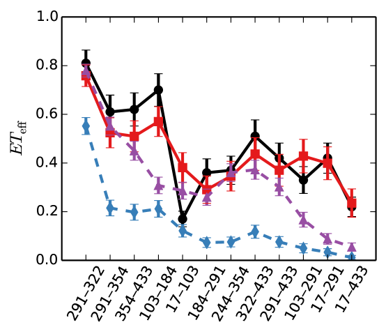
Figure 5: FRET efficiencies $ET_{\rm eff}$ for MAPT from smFRET experiments (black solid line with circles) and three CG simulations: 1) ${\overline{\epsilon}}_{a}=0$ and ${\overline{\epsilon}}_{es}=\kappa_{es}$ (blue diamonds), 2) the optimal $\alpha_{CG}=0.52$ with ${\overline{\epsilon}}_{es}=\kappa_{es}$, where the root-mean-square deviations between the experimental and simulation $ET_{\rm eff}$ are minimized (red squares), and 3) the optimal $\alpha_{CG}=0.52$ with no electrostatic interactions ${\overline{\epsilon}}_{es}=0$ (purple triangles).

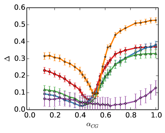
Figure 6: (Color online) Root-mean-square deviation $\Delta$ in $ET_{\rm eff}$ between experiments and simulations versus the ratio $\alpha_{CG}$ of the hydrophobicity and electrostatic interactions for $\alpha$S (red circles), $\beta$S (blue squares), and $\gamma$S (green triangles), MAPT (orange triangles), and ProT$\alpha$ (purple diamonds).

Sensitivity analysis of hydrophobicity models

In this section, we describe results from CG Langevin dynamics simulations of each IDP using $9$ different hydrophobicity models (Sec. 2): three hydrophobicity scales (the shifted and normalized Kyte-Doolittle [23] and Monera [28] scales, and an average of seven commonly used hydrophobicity scales) plus three pairwise mixing rules for the hydrophobicities of the residues (arithmetic mean, geometric mean, and maximum). For the CG simulations of each IDP and hydrophobicity model, we varied $\alpha_{CG}$ to minimize $\Delta$.

In Fig. 7, we show the root-mean-square (RMS) deviation in $ET_{\rm eff}$ between the simulations and experiment and the error in the RMS for each IDP and hydrophobicity model. We also show an estimate of the average error ($6$%) expected from the smFRET experiments [43]. For most of the hydrophobicity models, the RMS deviations in $ET_{\rm eff}$ between simulations and experiment for $\beta$S, $\gamma$S, and ProT$\alpha$ are below the experimental error. For $\alpha$S, most of the hydrophobicity models possess RMS deviations that are comparable to the experimental error. Thus, for the synuclein family and ProT$\alpha$, the RMS deviations are comparable or below experimental error and the hydrophobicity model does not strongly affect the results. For MAPT, the RMS deviations vary from $\Delta_{\rm min}\approx 0.08$ to $0.12$ indicating that some of the hydrophobicity models are slightly better than others for this IDP.

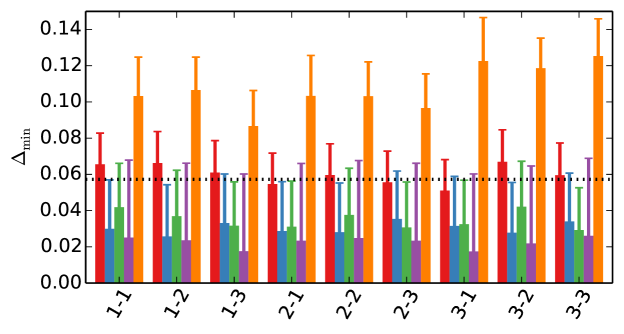
Figure 7: (Color online) RMS deviations $\Delta_{\rm min}$in $ET_{\rm eff}$ (and its error) between the experiments and simulations for (from left to right) $\alpha$S (red), $\beta$S (blue), $\gamma$S (green), ProT$\alpha$ (purple), and MAPT (orange) for 9 hydrophobicity models. The labeling scheme for the nine hydrophobicity models is (hydrophobicity scale)-(mixing rule) as numbered in Sec. 2. The RMS deviations are calculated from CG simulations with $\alpha_{CG}$ chosen such that the RMS deviations are minimized for each hydrophobicity scale and mixing rule. The black dotted line indicates the average error in $ET_{\rm eff}$ from smFRET experiments.

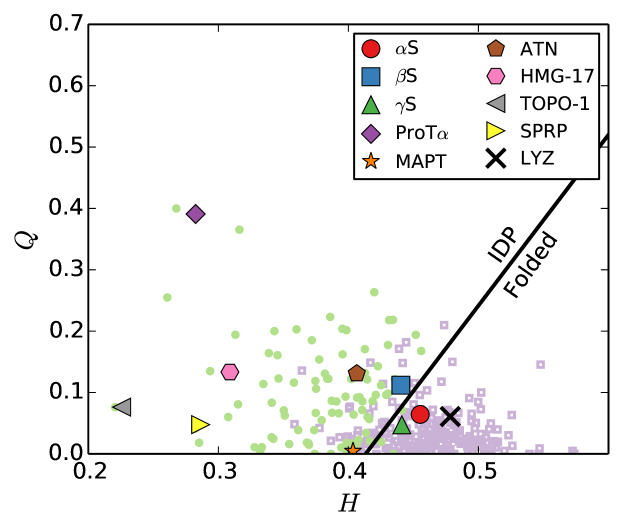
Figure 8: Absolute value of the electric charge per residue $Q$ versus the hydrophobicity per residue $H$ (using the shifted and normalized Monera hydrophobicity scale) for known IDPs (small circles) and $221$ folded proteins [45] (small open squares). The IDPs $\alpha$S (large circle), $\beta$S (large square), $\gamma$S (upward triangle), ProT$\alpha$ (diamond), MAPT (star), ATN (pentagon), HMG-17 (hexagon), TOPO-1 (leftward triangle), SPRP (rightward triangle), and the folded protein lysozyme C (X) are highlighted. The line $Q=2.785H-1.151$ represents the dividing line between IDPs (above the line) and natively folded proteins (below the line) given in Ref. [45].

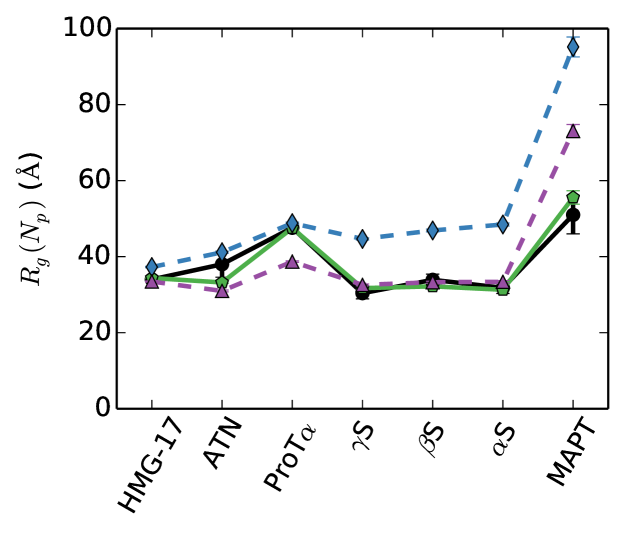
Figure 9: Radius of gyration $R_{g}(N_{p})$ of seven IDPs from experiments [22, 1, 14, 47, 31] (black circles) and simulations of three CG models: 1) $\epsilon_{a}=0$ and ${\overline{\epsilon}}_{es}=\kappa_{es}$ such that the chains behave as extended coils (blue diamonds), 2) $\alpha_{CG}=$0.50$$ and ${\overline{\epsilon}}_{es}=\kappa_{es}$ (green pentagons), and 3) $\alpha_{CG}=$0.50$$ and ${\overline{\epsilon}}_{es}=0$ (purple triangles). The IDPs are ordered from shortest to longest (left to right).

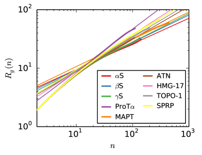
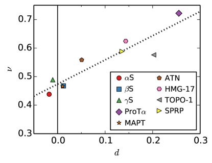
Figure 10: (left) Radius of gyration $R_{g}(n)$ (thick lines) versus chemical distance $n$ along the chain for several IDPs with $N\geq 90$ so that $R_{g}(n)$ is in the power-law scaling regime. Power-law fits of the data to $R_{g}=R^{0}n^{\nu}$ for $n>20$ are shown as thin lines. The error in $R_{g}$ is comparable to the line thickness. (right) Power-law scaling exponent $\nu$ as a function of the distance $d$ from the dividing line between folded and intrinsically disordered proteins (Fig. 8). The dotted line follows $\nu=0.47+0.85d$.

Scaling exponents

The charge-hydrophobicity plane [45] is a common rubric for differentiating natively folded and intrinsically disordered proteins. In Fig. 8, we plot the absolute value of the electric charge per residue $Q=N_{p}^{-1}|\sum_{i=1}^{N_{p}}Q_{i}|$ versus the hydrophobicity per residue $H=N_{p}^{-1}\sum_{i=1}^{N_{p}}\epsilon_{i}$ (using the shifted and normalized Monera hydrophobicity scale) for many known IDPs and folded proteins. We highlight $10$ specific proteins in Fig. 8: $\alpha$S, $\beta$S, $\gamma$S, ProT$\alpha$, high mobility anti-termination protein N (ATN), MAPT, non-histone chromosomal protein (HMG-17), DNA topoisomerase 1 (TOPO-1), basic salivary proline-rich protein 4 (SPRP), and lysosyme C (LYZ). The majority of IDPs occur above the line $Q=2.785H-1.151$, while natively folded proteins occur below the line. For example, the IDPs ProT$\alpha$ and HMG-17 occur significantly above the line, while the folded protein lysozyme C is well below the line. However, the synucleins and MAPT occur close to the dividing line between folded and intrinsically disordered proteins. In fact, $\alpha$S and $\gamma$S are on the folded-protein side of the dividing line along with several other IDPs, and thus the dividing line is somewhat ‘fuzzy’.

We seek to identify physical quantities that are able to distinguish the behavior of different IDPs. In this section, we employ the CG model to measure the radius of gyration $R_{g}$ as a function of chemical distance $n$ along the chain

$$R_{g}(n)=\frac{1}{N_{p}-n+1}\sum_{i=1}^{N_{p}-n}\left\langle R_{g}(i,i+n-1)\right\rangle_{t},$$ (10)

where $\left\langle.\right\rangle_{t}$ denotes a time average,

$$R_{g}(i,j)=\sqrt{\frac{1}{j-i+1}\sum_{k=i}^{j}\left({\vec{r}}_{k}-\left\langle{\vec{r}_{k}}\right\rangle\right)^{2}},$$ (11)

and

$$\left\langle{\vec{r}_{k}}\right\rangle=\frac{1}{j-i+1}\sum_{k=i}^{j}\vec{r}_{k},$$ (12)

for proteins over a broad range of the charge-hydrophobicity plane. In Fig. 9, we show the radius of gyration $R_{g}(N_{p})$ for seven IDPs (HMG-17, ATN, ProT$\alpha$, the synuclein family, and MAPT) ordered from shortest to longest. We find that the CG model with the optimal $\alpha_{CG}$ is able to recapitulate the experimental values of the radius of gyration for these IDPs to within approximately $10$%. We also show that the predicted $R_{g}(N_{p})$ from the CG model without electrostatics, ${\overline{\epsilon}}_{es}=0$, matches the experimental values for these IDPs, except for ProT$\alpha$ and MAPT. Additionally, the electrostatics-only model ($\alpha_{CG}=0$) is not able to recapitulate the experimental $R_{g}(N_{p})$ for most of these IDPs.

We show the dependence of $R_{g}(n)$ on the chemical distance $n$ along the chain for eight IDPs in Fig. 10 (left). For large $n$, $R_{g}$ displays power-law scaling, $R_{g}=R_{g}^{0}n^{\nu}$, where the scaling exponent $\nu$ varies from $\approx 0.5$ to $0.7$ as shown in Fig. 10 (right). We find that there is a strong correlation between $\nu$ and the distance $d$ of the protein from the dividing line between IDPs and folded proteins in the charge-hydrophobicity plane. For proteins near the dividing line, the exponent $\nu\approx 0.5$ shows ideal scaling, while swelling of the chain increases linearly with distance from the dividing line.

4 Conclusions

We developed a coarse-grained representation of intrinsically disordered proteins (IDPs) that includes steric, attractive hydrophobic, and screened electrostatic interactions between spherical residues. The CG model is calibrated to recapitulate a large set of experimental measurements of FRET efficiencies for $5$ IDPs and $36$ pairs of residues. We then performed Langevin dynamics simulations of the calibrated CG model to calculate the scaling of the radius of gyration with the chemical distance along the chain for a larger set of IDPs. We find a strong correlation between the scaling exponent $\nu$ that characterizes the swelling of the IDP and its distance from the line that separates IDPs and natively folded proteins in the hydrophobicity and charge plane. IDPs possess ideal scaling $(\nu\sim 0.5)$ near the dividing line, and the exponent increases linearly with distance from the dividing line. These results suggest that increasing the charge or decreasing hydrophobicity can have similar effects on the swelling of IDPs. In future studies, we will employ this simple, robust CG model to study the association and aggregation dynamics of tens to hundreds of IDPs and address such questions as: 1) Is the single-chain model for IDPs able to capture the aggregation of multiple IDPs, 2) Does $\beta$-sheet order form spontaneously in clusters of IDPs, and if so, 3) what is the critical nucleus for $\beta$-sheet order?

References

- Abercrombie et al. [1978] Abercrombie, B. D., Kneale, G. G., Crane-Robinson, C., Bradbury, E. M., Goodwin, G. H., Walker, J. M., and Johns, E. W., European journal of biochemistry / FEBS 84, 173 (1978).
- Allen and Tildesley [1989] Allen, M. P. and Tildesley, D. J., Computer simulation of liquids (Oxford University Press, 1989).
- Brooks et al. [2009] Brooks, B. R., Brooks, C. L., MacKerell, A. D., Nilsson, L., Petrella, R. J., Roux, B., Won, Y., Archontis, G., Bartels, C., Boresch, S., et al., Journal of computational chemistry 30, 1545 (2009).
- Castanon et al. [1988] Castanon, M., Spevak, W., Adolf, G., Chlebowicz-Sledziewska, E., and Sledziewski, A., Gene 66, 223 (1988).
- Clementi [2008] Clementi, C., Current opinion in structural biology 18, 10 (2008).
- Cornette et al. [1987] Cornette, J. L., Cease, K. B., Margalit, H., Spouge, J. L., Berzofsky, J. A., and DeLisi, C., Journal of molecular biology 195, 659 (1987).
- Dedmon et al. [2005] Dedmon, M. M., Lindorff-Larsen, K., Christodoulou, J., Vendruscolo, M., and Dobson, C. M., Journal of the American Chemical Society 127, 476 (2005).
- Dobson [2003] Dobson, C. M., Nature 426, 884 (2003).
- Ducas and Rhoades [2014] Ducas, V. C. and Rhoades, E., PLOS ONE 9, e86983 (2014).
- Dunker et al. [2001] Dunker, A., Lawson, J., Brown, C. J., Williams, R. M., Romero, P., Oh, J. S., Oldfield, C. J., Campen, A. M., Ratliff, C. M., Hipps, K. W., Ausio, J., Nissen, M. S., Reeves, R., Kang, C., Kissinger, C. R., Bailey, R. W., Griswold, M. D., Chiu, W., Garner, E. C., and Obradovic, Z., Journal of Molecular Graphics and Modelling 19, 26 (2001).
- Dyson and Wright [2005] Dyson, H. J. and Wright, P. E., Nature reviews. Molecular cell biology 6, 197 (2005).
- Eisenberg et al. [1984] Eisenberg, D., Schwarz, E., Komaromy, M., and Wall, R., Journal of molecular biology 179, 125 (1984).
- Eschenfeldt and Berger [1986] Eschenfeldt, W. H. and Berger, S. L., Proceedings of the National Academy of Sciences 83, 9403 (1986).
- Gast et al. [1995] Gast, K., Damaschun, H., Eckert, K., Schulze-Forster, K., Maurer, H. R., Mueller-Frohne, M., Zirwer, D., Czarnecki, J., and Damaschun, G., Biochemistry 34, 13211 (1995).
- Giehm et al. [2011] Giehm, L., Svergun, D. I., Otzen, D. E., and Vestergaard, B., Proceedings of the National Academy of Sciences 108, 3246 (2011).
- Goedert et al. [1989] Goedert, M., Spillantini, M., Jakes, R., Rutherford, D., and Crowther, R., Neuron 3, 519 (1989).
- Goedert et al. [1988] Goedert, M., Wischik, C., Crowther, R., Walker, J., and Klug, A., Proceedings of the National Academy of Sciences 85, 4051 (1988).
- Hashimoto et al. [2001] Hashimoto, M., Rockenstein, E., Mante, M., Mallory, M., and Masliah, E., Neuron 32, 213 (2001).
- Hofmann et al. [2012] Hofmann, H., Soranno, A., Borgia, A., Gast, K., Nettels, D., and Schuler, B., Proceedings of the National Academy of Sciences of the United States of America 109, 16155 (2012).
- Jakes, Spillantini, and Goedert [1994] Jakes, R., Spillantini, M. G., and Goedert, M., FEBS letters 345, 27 (1994).
- Ji et al. [1997] Ji, H., Liu, Y. E., Jia, T., Liu, Y. E., Xiao, G., Joseph, K., Rosen, C., and Sm, Y. E., Cancer Res 57, 759 (1997).
- Johansen et al. [2011] Johansen, D., Jeffries, C. M. J., Hammouda, B., Trewhella, J., and Goldenberg, D. P., Biophysical journal 100, 1120 (2011).
- Kyte and Doolittle [1982] Kyte, J. and Doolittle, R. F., Journal of molecular biology 157, 105 (1982).
- Li, Uversky, and Fink [2002] Li, J., Uversky, V. N., and Fink, A. L., NeuroToxicology 23, 553 (2002).
- Mao et al. [2010] Mao, A. H., Crick, S. L., Vitalis, A., Chicoine, C. L., and Pappu, R. V., Proceedings of the National Academy of Sciences of the United States of America 107, 8183 (2010).
- Mittag and Forman-Kay [2007] Mittag, T. and Forman-Kay, J. D., Current opinion in structural biology 17, 3 (2007).
- Miyazawa and Jernigan [1985] Miyazawa, S. and Jernigan, R. L., Macromolecules 18, 534 (1985).
- Monera et al. [1995] Monera, O. D., Sereda, T. J., Zhou, N. E., Kay, C. M., and Hodges, R. S., Journal of peptide science : an official publication of the European Peptide Society 1, 319 (1995).
- Morar et al. [2001] Morar, A. S., Olteanu, A., Young, G. B., and Pielak, G. J., Protein Science 10, 2195 (2001).
- Müller-Späth et al. [2010] Müller-Späth, S., Soranno, A., Hirschfeld, V., Hofmann, H., Rüegger, S., Reymond, L., Nettels, D., and Schuler, B., Proceedings of the National Academy of Sciences 107, 14609 (2010).
- Nath et al. [2012] Nath, A., Sammalkorpi, M., DeWitt, D., Trexler, A., Elbaum-Garfinkle, S., O’Hern, C., and Rhoades, E., Biophys. J. 103, 1940 (2012).
- Nath et al. [2010] Nath, S., Meuvis, J., Hendrix, J., Carl, S. A., and Engelborghs, Y., Biophysical Journal 98, 1302 (2010).
- Oostenbrink et al. [2004] Oostenbrink, C., Villa, A., Mark, A. E., and van Gunsteren, W. F., Journal of computational chemistry 25, 1656 (2004).
- Rekas et al. [2010] Rekas, A., Knott, R., Sokolova, A., Barnham, K., Perez, K., Masters, C., Drew, S., Cappai, R., Curtain, C., and Pham, C., European Biophysics Journal 39, 1407 (2010).
- Salmon et al. [2010] Salmon, L., Nodet, G., Ozenne, V., Yin, G., Jensen, M. R., Zweckstetter, M., and Blackledge, M., Journal of the American Chemical Society 132, 8407 (2010).
- Salomon-Ferrer, Case, and Walker [2013] Salomon-Ferrer, R., Case, D. A., and Walker, R. C., Wiley Interdisciplinary Reviews: Computational Molecular Science 3, 198 (2013).
- Sharp et al. [1991] Sharp, K. A., Nicholls, a., Friedman, R., and Honig, B., Biochemistry 30, 9686 (1991).
- Smith et al. [2012] Smith, W. W., Schreck, C. F., Hashem, N., Soltani, S., Nath, A., Rhoades, E., and O’Hern, C. S., Physical Review E 86, 041910 (2012).
- Sugase, Dyson, and Wright [2007] Sugase, K., Dyson, H. J., and Wright, P. E., Nature 447, 1021 (2007).
- Szilágyi, Györffy, and Závodszky [2008] Szilágyi, A., Györffy, D., and Závodszky, P., Biophysical journal 95, 1612 (2008).
- Tashiro et al. [2008] Tashiro, M., Kojima, M., Kihara, H., Kasai, K., Kamiyoshihara, T., Uéda, K., and Shimotakahara, S., Biochemical and Biophysical Research Communications 369, 910 (2008).
- Trexler and Rhoades [2013] Trexler, A. and Rhoades, E., Mol. Neurobiol. 47, 622 (2013).
- Trexler and Rhoades [2010] Trexler, A. J. and Rhoades, E., Biophysical journal 99, 3048 (2010).
- Uéda et al. [1993] Uéda, K., Fukushima, H., Masliah, E., Xia, Y., Iwai, a., Yoshimoto, M., Otero, D. a., Kondo, J., Ihara, Y., and Saitoh, T., Proceedings of the National Academy of Sciences of the United States of America 90, 11282 (1993).
- Uversky, Gillespie, and Fink [2000] Uversky, V. N., Gillespie, J. R., and Fink, A. L., Proteins 41, 415 (2000).
- Uversky, Li, and Fink [2001] Uversky, V. N., Li, J., and Fink, A. L., FEBS Letters 509, 31 (2001).
- Uversky et al. [2002] Uversky, V. N., Li, J., Souillac, P., Millett, I. S., Doniach, S., Jakes, R., Goedert, M., and Fink, A. L., The Journal of biological chemistry 277, 11970 (2002).
- Uversky et al. [2005] Uversky, V. N., Yamin, G., Munishkina, L. A., Karymov, M. A., Millett, I. S., Doniach, S., Lyubchenko, Y. L., and Fink, A. L., Molecular Brain Research 134, 84 (2005).
- Vucetic et al. [2003] Vucetic, S., Brown, C. J., Dunker, A. K., and Obradovic, Z., Proteins 52, 573 (2003).
- Wang and Dunbrack [2003] Wang, G. and Dunbrack, R. L., Bioinformatics 19, 1589 (2003), pMID: 12912846.
- White and Wimley [1999] White, S. H. and Wimley, W. C., Annual review of biophysics and biomolecular structure 28, 319 (1999).
- Wimley and White [1996] Wimley, W. C. and White, S. H., Nature Structural Biology 3, 842 (1996).