Multiphoton resonances for all optical quantum logic with multiple cavities

Abstract

We develop a theory for the interaction of multi-level atoms with multi-mode cavities yielding cavity-enhanced multi-photon resonances. The locations of the resonances are predicted from the use of effective two- and three-level Hamiltonians. As an application we show that quantum gates can be realised when photonic qubits are encoded on the cavity modes in arrangements where ancilla atoms transit the cavity. The fidelity of operations is increased by conditional measurements on the atom and by the use of a selected, dual-rail, Hilbert space. A universal set of gates is proposed, including the Fredkin gate and iswap operation; the system seems promising for scalability.

I Introduction

The field of quantum computation Nielsen and Chuang (2000) has attracted proposals for many different physical realisations. Amongst these, the use of photonic qubits is appealing because of the potential interface to optical communications, the accessibility of coherent sources for qubits and the possibility of manipulating those qubits using established optical technology. With photonic qubits a central issue is that of enabling sufficiently strong, and coherent, interactions for quantum logic. The field of cavity QED (or CQED) naturally meets these requirements as it has a history of coherent quantum interactions and entanglement generation Raimond et al. (2001); Walther et al. (2006). Alternatively, non-linear media can be used for qubit interactions, but very strong non-linearities are needed for the non-linear media (see e.g. Refs. Milburn (1989); Yavuz (2005); O’Brien (2007)). The approach of linear optical computing Knill et al. (2001), which uses passive optical components, can be used and seems promising Kok et al. (2007), although the use of “flying qubits,” generally pulses encoded in polarisation states, can make the approach susceptible to photon losses O’Brien (2007), and it also places high demands on single-photon sources.

With CQED a single photon can have a strong interaction with an atom, which usually results in at least a two step process for interactions between photonic qubits. This approach has been used for quantum logic with, for example, flying photonic qubits and cavities Duan and Kimble (2004), with qubits in atoms that talk via a cavity mode “bus” Pellizzari et al. (1995), and with qubits in both the atoms and the cavity modes Rauschenbeutel et al. (1999); Lin et al. (2006); Biswas and Agarwal (2004); Joshi and Xiao (2006). If we wanted to avoid the losses associated with flying photonic qubits, and use cavity storage of photons, we can still use CQED with an atom “bus”. Examples typically involve two cavity modes (with qubits represented as the absence or presence of a photon) and three-level, or more complex, atoms (see e.g. Zubairy et al. (2003); Shu et al. (2007); Lin et al. (2008)).

Existing methods for quantum logic with stored cavity photons do not, to our knowledge, use the advantageous “dual-rail” channel Chuang and Yamamoto (1995); Kok et al. (2007). With flying qubits the dual-rail approach means that a qubit is typically encoded as a single-photon pulse in one of two polarisations. This means that qubit loss is detected by the absence of a photon. We will adapt this approach to cavity stored photons by encoding a single qubit on a pair of cavity field modes. The presence of excitation in a first mode (no excitation in the second) encodes the $\left|1\right\rangle$ qubit state, and the presence of excitation in the second mode encodes a qubit state $\left|0\right\rangle$ (see Table 1).

Modes		Qubit
$\left|1\right\rangle$$\left|0\right\rangle$	$\mapsto$	$\left|1\right\rangle$
$\left|0\right\rangle$$\left|1\right\rangle$	$\mapsto$	$\left|0\right\rangle$

Table 1: A qubit is encoded as a single excitation shared between two modes of the field. A logical one maps to the excitation residing fully in the first mode, and the logical zero maps to the excitation being fully in the second mode.

Thus superpositions of qubit states will involve entangled states of the cavity modes. In Sec. V of this paper we show how to achieve the $x$-rotation of single logical qubits which can be arranged to ensure that, for example, $\left|0\right\rangle\longrightarrow(\left|0\right\rangle+\left|1\right\rangle)/\sqrt{2}$. However, in terms of physical states, an entangled state $(\left|01\right\rangle+\left|10\right\rangle)/\sqrt{2}$ has been created. There has been considerable interest in such states recently in terms of the decay of entanglement Bellomo et al. (2007); Maniscalco et al. (2008); Wang et al. (2008); Li et al. (2009); Mazzola et al. (2009a); Zhou et al. (2009); Ferraro et al. (2009); Francica et al. (2009); Xiao et al. (2009); Zhang et al. (2009); Mazzola et al. (2009b, 2010a, 2010b); Fanchini et al. (2010); Tong et al. (2010); Wang et al. (2010); Man et al. (2010). The $x$-rotation procedure would create such an entangled state with photons in independent reservoirs. An interesting feature of the qubit encoding (Table 1) is that, if any excitation is lost, then the resulting state of the pair of modes, $\left|0\right\rangle\left|0\right\rangle$, does not map to a valid qubit. In this way quantum information processing amounts to the rearrangement of photons in our system.

The clear disadvantage of this approach, in a CQED implementation, is that the duplexity of cavity modes increases the difficulty of formulating gates, and increases the vulnerability to cavity decay. The purpose of this paper is to show that, nevertheless, a practical and universal set of gates can be found for dual-rail qubits in a CQED system using strong coupling. We will see that the rearrangement of photons is performed by an ancilla atom which enters and then leaves the multi-mode cavity (see Fig. 1).

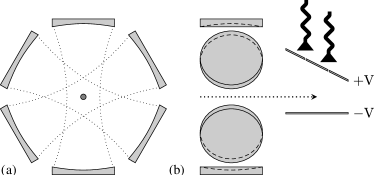
Figure 1: Simplified illustration of the physical layout of a single gate of the type considered in the Paper. Axial (a) and side (b) views are shown. A single atom enters a multi-mode cavity and interacts with the photonic qubits present. An interaction with as many as six cavity modes is considered. On exit from the cavities, the atomic state is measured. The illustration shows state selective field ionization Meschede et al. (1985) as an example. The measurement allows us to enhance the fidelity of the gate operation.

Because the quantum information resides in the cavity modes, the ancilla atom must leave in an un-entangled state. (This is the inverse of the case where two atoms interact with a detuned cavity field to produce entanglement between the atoms, while remaining un-entangled with the field Zheng and Guo (2000); Osnaghi et al. (2001).) We can “help” the disentanglement by performing a measurement on the atom when it has left the cavity. The measurement is intended to “clean up” the quantum state, i.e. the probability of failure is low, and the ensuing projection assists the gate fidelity. This approach is reminiscent of that used to create Fock states by means of a sequence of conditional measurements Garraway et al. (1994). In this sense the role of the measurement is quite different to the continuous measurement schemes used in some logic gates (see e.g. Refs. Pellizzari et al. (1995); Franson et al. (2004)): here it is more a helpful herald.

The gates in this paper are based on multi-photon resonances that involve cavity mode photons distributed amongst several modes. The absence of a photon in a mode can break the chain of resonant interaction: this is the key to the quantum logic processes we study. To analyse the multi-photon resonances themselves, we adapt a technique of adiabatic elimination from atomic physics Shore (1981). However, rather than using a chain of atomic states coupled by coherent fields, we use a chain of coupled cavity-atom states coupled with small numbers of photons.

In the following we first briefly set up the general multi-level and multi-mode system in Sec. II, and then give a simple application to an iswap gate in Sec. III. In Sec. IV, which contains the main results of the paper, we use the theory of effective Hamiltonians Shore (1981) to describe the multi-photon operation of a Fredkin gate. Two Fredkin gate schemes are presented: the first (Sec. IV.1) illustrates the basic ideas and the second approach (presented in Sec. IV.2) improves the operation of the gate. Details of the adiabatic elimination procedures are in the Appendices. In Sec. V we find that it is possible to realize the $x$-rotation and $z$-rotation gates, which together with the Fredkin gate, form a universal set Nielsen and Chuang (2000). The paper concludes with Sec. VI where we also discuss the scalability of the proposed scheme.

II The multi-level model

At the heart of the atom-field interactions is the generic multi-level and multi-mode Hamiltonian ($\hbar=1$)

$$H = \sum_{i,\alpha,\beta}H_{i}^{\alpha\beta}$$

$$= \sum_{i,\alpha,\beta}E_{\beta}\hat{\sigma}_{\mathrm{\beta\beta}}+E_{\alpha}\hat{\sigma}_{\mathrm{\alpha\alpha}}+\omega_{i}\hat{a}^{\dagger}_{i}\hat{a}_{i}+g^{\mathrm{\alpha\beta}}_{i}\left(\hat{a}_{i}\hat{\sigma}_{\mathrm{\alpha\beta}}+\hat{a}^{\dagger}_{i}\hat{\sigma}_{\mathrm{\beta\alpha}}\right)$$

where a mode of frequency $\omega_{i}$ is coupled to two atomic levels $\left|\alpha\right\rangle$, $\left|\beta\right\rangle$, with energies $E_{\alpha}$ and $E_{\beta}$ (with $E_{\alpha}>E_{\beta}$). The coupling strength is $g^{\mathrm{\alpha\beta}}_{i}$, and the atomic operators $\hat{\sigma}_{\mathrm{\alpha\beta}}\equiv\left|\alpha\right\rangle\left\langle\beta\right|$. For multi-mode fields and multilevel atoms we will have many possibilities for selecting the modes and atomic states. We will assume that any given pair of atomic levels either couples to a single cavity mode or is extremely non-resonant, and that the Hamiltonian for the system can be written as the sum of terms Eq. (II).

Before analyzing the iswap and Fredkin gates in detail in Secs. III and IV, we start with a brief illustration of the concepts of the swapping process with cavity excitations as depicted for iswap with a double-lambda scheme as shown in Fig. 2. Consider the case of the initial state of the system such that the atom is in the state $\left|a\right\rangle$, modes one and three both have a single excitation, and modes two and four have no excitations (so that the overall state can be represented by $\left|1010,a\right\rangle$). Then the system can resonantly oscillate between the initial state and the state where the excitations have been moved to modes two and four: i.e. it oscillates between $\left|1010,a\right\rangle$ and $\left|0101,a\right\rangle$ if $\Delta_{4}\rightarrow 0$. Three other states of the system, $\left|0010,b\right\rangle$, $\left|0110,c\right\rangle$ and $\left|0100,d\right\rangle$ are also accessible. To stop states of the atom other than $\left|a\right\rangle$ being populated the transitions may be detuned, i.e. detunings $\Delta_{1,2,3}$ are large. If we have the limit $\Delta_{4}\rightarrow 0$, then only the two states of interest, $\left|1010,a\right\rangle$ and $\left|0101,a\right\rangle$ may be populated. The price to be paid for detuning the intermediate states is a slower gate, as we will see in the Section IV when we analyze the six-mode Fredkin gate. If the two excitations in the system are initially in either of the alternate configurations $\left|1001,a\right\rangle$ or $\left|0110,a\right\rangle$ then no movement of excitations can occur as the large detuning of the intermediate states makes this energetically unfavorable. If we apply the encoding of a qubit, as in Table 1, this system can map qubits onto an iswap gate as seen in detail in the next section.

Figure 2: A double-lambda scheme with four modes and four atomic levels, which can form an iswap gate for photonic qubits (section III). At certain interaction times this leads to a rearrangement of excitations between the cavity modes without a resulting excitation of the atom. The detunings $\Delta_{i}$ represent the detuning of virtual states in the multi-photon resonance found when $\Delta_{4}\sim 0$.

III iswap gate

III.1 Configuration for a basic iswap gate

Given an atomic system of energy levels coupled to two dual rail qubits as shown in Fig. 2, we have seen that it may be possible to limit the system to two essential states which will oscillate. The resulting interaction is equivalent to an iswap gate Schuch and Siewert (2003) which is shown in Table 2.

First we map four possible initial states of the system to qubits as in Table 1:

$$\begin{split}\left|0110,a\right\rangle&\mapsto\left|00,a\right\rangle\\ \left|0101,a\right\rangle&\mapsto\left|01,a\right\rangle\\ \left|1010,a\right\rangle&\mapsto\left|10,a\right\rangle\\ \left|1001,a\right\rangle&\mapsto\left|11,a\right\rangle\,,\end{split}$$ (2)

where the $a$ is a reminder that the atom is always entered in state $\left|a\right\rangle$.

Input		Output
$\left|00\right\rangle$		$\left|00\right\rangle$
$\left|01\right\rangle$		i$\left|10\right\rangle$
$\left|10\right\rangle$		i$\left|01\right\rangle$
$\left|11\right\rangle$		$\left|11\right\rangle$

Table 2: Truth table for the iswap gate Schuch and Siewert (2003). The iswap gate is locally equivalent to a combined cnot and swap operation Schuch and Siewert (2003), and forms a universal set with the one qubit rotation gates.

The Hamiltonian for this system in an interaction picture for the logical states $\left|01\right\rangle$ and $\left|10\right\rangle$ is

$$\begin{split}H_{I}=&-\Delta_{1}\hat{n}_{1}+g^{\mathrm{ab}}_{1}\left(\hat{a}_{1}\hat{\sigma}_{\mathrm{ba}}+\hat{a}^{\dagger}_{1}\hat{\sigma}_{\mathrm{ab}}\right)\\ &+(\Delta_{2}-\Delta_{1})\hat{n}_{2}+g^{\mathrm{bc}}_{2}\left(\hat{a}_{2}\hat{\sigma}_{\mathrm{bc}}+\hat{a}^{\dagger}_{2}\hat{\sigma}_{\mathrm{cb}}\right)\\ &+(\Delta_{2}-\Delta_{3})\hat{n}_{3}+g^{\mathrm{cd}}_{3}\left(\hat{a}_{3}\hat{\sigma}_{\mathrm{dc}}+\hat{a}^{\dagger}_{3}\hat{\sigma}_{\mathrm{cd}}\right)\\ &+(\Delta_{4}-\Delta_{3})\hat{n}_{4}+g^{\mathrm{da}}_{4}\left(\hat{a}_{4}\hat{\sigma}_{\mathrm{da}}+\hat{a}^{\dagger}_{4}\hat{\sigma}_{\mathrm{ad}}\right).\\ \end{split}$$ (3)

The derivation of this Hamiltonian may be found in Appendix A. By choosing $\Delta_{1,2,3}\gg(g^{\mathrm{ab}}_{1},g^{\mathrm{bc}}_{2},g^{\mathrm{cd}}_{3},g^{\mathrm{da}}_{4},\Delta_{4})$ a two-level effective Hamiltonian may also be derived as shown in Appendix A. This amounts to an adiabatic elimination of off-resonant states. The effective Hamiltonian operates on two qubit states of the system, i.e. $\left|10\right\rangle$$\left|a\right\rangle$ and $\left|01\right\rangle$$\left|a\right\rangle$. The effective Hamiltonian takes the form

$$H_{\mathrm{eff}}=\hat{\sigma}^{+}\hat{\sigma}^{-}\Delta_{\mathrm{eff}}+g_{\mathrm{eff}}\left(\hat{\sigma}^{+}+\hat{\sigma}^{-}\right)\,,$$ (4)

where $\hat{\sigma}^{+}=\left|01,a\right\rangle\left\langle 10,a\right|$, $\hat{\sigma}^{-}=\left|10,a\right\rangle\left\langle 01,a\right|$ and

$$\Delta_{\mathrm{eff}} \simeq\Delta_{4}-\frac{(g^{\mathrm{da}}_{4})^{2}}{\Delta_{3}}+\frac{(g^{\mathrm{ab}}_{1})^{2}}{\Delta_{1}}$$ (5)

$$g_{\mathrm{eff}} \simeq-\frac{g^{\mathrm{ab}}_{1}g^{\mathrm{bc}}_{2}g^{\mathrm{cd}}_{3}g^{\mathrm{da}}_{4}}{\Delta_{1}\Delta_{2}\Delta_{3}}\,.$$ (6)

The time evolution of the system for the states of interest is then given by

$$\begin{split}\left|10,a\right\rangle&\mapsto\cos(g_{\mathrm{eff}}t)\left|10,a\right\rangle-i\sin(g_{\mathrm{eff}}t)\left|01,a\right\rangle\\ \left|01,a\right\rangle&\mapsto\cos(g_{\mathrm{eff}}t)\left|01,a\right\rangle-i\sin(g_{\mathrm{eff}}t)\left|10,a\right\rangle\,,\end{split}$$ (7)

and the two other logical states of the system, $\left|00\right\rangle$ and $\left|11\right\rangle$ are unchanged as there are no resonant interactions and the detunings $\Delta_{1,2,3}$ are large. By choosing an appropriate interaction time ($|g_{\mathrm{eff}}t|=\pi/2$) an iswap gate operation is realized.

Unfortunately this gate is relatively slow, as it depends on a four photon process. Assuming that a typical detuning $\Delta_{i}$ should be an order of magnitude larger than a typical coupling constant $g_{j}$ to make the effective Hamiltonian a good approximation, the effective coupling constant $g_{\mathrm{eff}}$ will be three orders of magnitude smaller than a typical coupling constant. In a micromaser-like system with a coupling $g_{j}/(2\pi)\approx 10^{4}$ Hz and a quality factor $Q\approx 10^{10}$ at $\omega/(2\pi)\approx 10^{10}$ Hz Walther et al. (2006) the gate time will only be an order of magnitude smaller than the decay time of the cavity.

IV Multi-photon Fredkin gate

IV.1 Configuration for a basic multi-photon Fredkin gate

In order to build up a complete set of gates for dual-rail CQED QIP we need a faster gate than the iswap gate which also entangles qubits, such as the multi-qubit entangling Fredkin gate. To form this gate we actually add two more transitions to the iswap gate configuration. This trades a four photon process for a six photon process that will be slower, but in section IV.2 we show that a faster gate can be produced by allowing another state of the system to be resonant. These extra transitions both couple to the same mode, so that the presence of a photon in this additional mode is required to enable the swap interaction in the remaining modes, and its absence will prohibit the interaction. In this way we will realize a Fredkin gate Nielsen and Chuang (2000); Everitt and Garraway (2007). Figure 3 shows how the transitions and modes can be arranged to facilitate this. Making a transition from $\left|a\right\rangle$ completely around the loop of atomic states will absorb the photon from mode one, and then return it.

To understand the full dynamics in detail, we write the Hamiltonian of the system in an interaction picture as

$$\begin{split}H_{I}=&-\Delta_{1}\hat{n}_{1}+g^{\mathrm{ab}}_{1}\left(\hat{a}_{1}\hat{\sigma}_{\mathrm{ba}}+\hat{a}^{\dagger}_{1}\hat{\sigma}_{\mathrm{ab}}\right)\\ &+(\Delta_{2}-\Delta_{1})\hat{n}_{2}+g^{\mathrm{bc}}_{2}\left(\hat{a}_{2}\hat{\sigma}_{\mathrm{bc}}+\hat{a}^{\dagger}_{2}\hat{\sigma}_{\mathrm{cb}}\right)\\ &+(\Delta_{2}-\Delta_{3})\hat{n}_{3}+g^{\mathrm{cd}}_{3}\left(\hat{a}_{3}\hat{\sigma}_{\mathrm{dc}}+\hat{a}^{\dagger}_{3}\hat{\sigma}_{\mathrm{cd}}\right)\\ &+\left(\hat{n}_{1}+\hat{n}_{2}+\hat{n}_{3}+\hat{n}_{6}-\hat{\sigma}_{\mathrm{aa}}-\hat{\sigma}_{\mathrm{cc}}\right)(\Delta_{1}-\Delta_{3}+\Delta_{4})\\ &+g^{\mathrm{de}}_{1}\left(\hat{a}_{1}\hat{\sigma}_{\mathrm{de}}+\hat{a}^{\dagger}_{1}\hat{\sigma}_{\mathrm{ed}}\right)\\ &+(\Delta_{4}-\Delta_{5})\hat{n}_{5}+g^{\mathrm{ef}}_{5}\left(\hat{a}_{5}\hat{\sigma}_{\mathrm{fe}}+\hat{a}^{\dagger}_{5}\hat{\sigma}_{\mathrm{ef}}\right)\\ &+(\Delta_{6}-\Delta_{5})\hat{n}_{6}+g^{\mathrm{fa}}_{6}\left(\hat{a}_{6}\hat{\sigma}_{\mathrm{fa}}+\hat{a}^{\dagger}_{6}\hat{\sigma}_{\mathrm{af}}\right)\end{split}$$ (8)

where $\hat{n}_{i}=\hat{a}^{\dagger}_{i}\hat{a}_{i}$. Details can be found in Appendix B.1 where we have carefully chosen the basis to make the Hamiltonian time independent. An overall energy shift has been neglected, and the detunings $\Delta_{j}$ are as shown in Fig. 3.

Our aim of rearranging excitations in the target modes ($\omega_{2},\omega_{3},\omega_{5},\omega_{6}$) could be achieved by having the resonant case (all $\Delta_{i}=0$), but this is a rather special case which is very sensitive to decoherence. The optimization of the gate operation has turned out to be an interesting problem with a number of different solutions. Another approach would be to aim for a multiphoton resonance: i.e. $\Delta_{6}=0$ with large detunings $\Delta_{1\mbox{--}5}$ (see Fig. 3). We could then use an effective two-level Hamiltonian Cook and Shore (1979); Shore (1981) to model the dynamics of the whole system as if it were an atomic ladder (see Appendix B.2). However, an important difference here is that the state space of the system involves both atomic states and quantized cavity field states.

Figure 3: The level scheme, with repeated mode $\omega_{1}$, which can realize a Fredkin (controlled swap) gate when $\Delta_{6}\sim 0$ (multiphoton resonance). The mode $\omega_{4}$ is not shown here. By tuning $\Delta_{3}$ according to the resonance conditions (16) the operational speed of the gate can be increased.

To encode the qubits, the first mode ($\omega_{1}$) is paired up with a mode ($\omega_{4}$) that is not resonant with any transition and does not appear in Fig. 3. If we then label the other modes as shown in Fig. 3, we have three logical qubits represented as

$$\left|q_{1},q_{2},q_{3}\right\rangle\equiv\left|n_{1}n_{4},n_{2}n_{3},n_{5}n_{6}\right\rangle.$$ (9)

Only two states of the qubit system are effectively resonant, i.e. a coupling exists between the logical states

$$\left|101,a\right\rangle\leftrightarrow\left|110,a\right\rangle\,,$$ (10)

and the six remaining configurations of qubits (listed in Table 3) do not make transitions. The two states in Eq. (10) are coupled via five other intermediate atom-field states. Close to the multi-photon resonance we can produce an effective two-level Hamiltonian Shore (1981). The derivation may be found in Appendix B.2 and the effective Hamiltonian is

$$H_{\mathrm{eff}}=\hat{\sigma}^{+}\hat{\sigma}^{-}\Delta_{\mathrm{eff}}+g_{\mathrm{eff}}\left(\hat{\sigma}^{+}+\hat{\sigma}^{-}\right)$$ (11)

where $\hat{\sigma}^{+}\equiv\left|110,a\right\rangle\left\langle 101,a\right|$ and the atomic state could be factored out from the effective Hamiltonian. The effective coupling is

$$g_{\mathrm{eff}}\simeq-\frac{g^{\mathrm{ab}}_{1}g^{\mathrm{bc}}_{2}g^{\mathrm{cd}}_{3}g^{\mathrm{de}}_{1}g^{\mathrm{ef}}_{5}g^{\mathrm{fa}}_{6}}{\Delta_{1}\Delta_{2}\Delta_{3}\Delta_{4}\Delta_{5}}$$ (12)

and the resonance condition, which has gained a component due to level shifts, is

$$\Delta_{\mathrm{eff}}\simeq\Delta_{6}-\frac{\left(g^{\mathrm{fa}}_{6}\right)^{2}}{\Delta_{5}}\,.$$ (13)

We can now see that the condition for resonance is only very approximately $\Delta_{6}=0$ and we should actually use $\Delta_{\mathrm{eff}}=0$ which implies $\Delta_{6}\simeq(g^{\mathrm{fa}}_{6})^{2}/\Delta_{5}$. Thus the evolution of the system, initially in the state $\left|101,a\right\rangle$ or $\left|110,a\right\rangle$, is effectively

$$\begin{split}\left|101,a\right\rangle&\mapsto\cos(g_{\mathrm{eff}}t)\left|101,a\right\rangle-i\sin(g_{\mathrm{eff}}t)\mathrm{e}^{i\eta t}\left|110,a\right\rangle\\ \left|110,a\right\rangle&\mapsto\cos(g_{\mathrm{eff}}t)\left|110,a\right\rangle-i\sin(g_{\mathrm{eff}}t)\mathrm{e}^{i\eta t}\left|101,a\right\rangle,\end{split}$$ (14)

where to obtain the exact Fredkin gate truth table (Table 3) without phase factors, we have undone the $\hat{\Theta}_{2}$ transformation of Appendix B.1. Then a phase factor depending on

$$\eta=\Delta_{1}-\Delta_{3}+\Delta_{4}\,.$$ (15)

appears in Eq. (14) which amounts to trivially changing the phase of the couplings.

Input		Output
$\left|000\right\rangle$		$\left|000\right\rangle$
$\left|001\right\rangle$		$\left|001\right\rangle$
$\left|010\right\rangle$		$\left|010\right\rangle$
$\left|011\right\rangle$		$\left|011\right\rangle$
$\left|100\right\rangle$		$\left|100\right\rangle$
$\left|110\right\rangle$		$\left|101\right\rangle$
$\left|101\right\rangle$		$\left|110\right\rangle$
$\left|111\right\rangle$		$\left|111\right\rangle$

Table 3: Truth table for the effective two-level system with $|g_{\mathrm{eff}}t|=\pi/2$ and $\eta t=\pi/2$ [see Eq. (14)] which produces a Fredkin gate Nielsen and Chuang (2000).

For effective operation, a typical coupling constant in Eq. (8) must be at least an order of magnitude smaller than its associated detuning. This implies that the effective coupling constant $g_{\mathrm{eff}}$ would be five orders of magnitude smaller than a typical cavity coupling constant, which would leave the interaction prohibitively slow, even in modern cavities. We will improve this coupling constant with the approach given in the next section.

IV.2 Configuration for a fast multi-photon Fredkin gate

To improve significantly the performance of the gate we allow the transitions to level $\left|d\right\rangle$ to be resonant (see Fig. 3). This gives a useful compromise between sensitivity and an improved gate operating time. We extend the effective Hamiltonian method of Ref. Shore (1981) to a three-level case as indicated in Appendix B.3. Then the conditions for resonance are:

$$\begin{split}&\Delta_{3}\simeq\frac{\left(g^{\mathrm{cd}}_{3}\right)^{2}}{\Delta_{2}}+\frac{\left(g^{\mathrm{de}}_{1}\right)^{2}}{\Delta_{4}}-\frac{\left(g^{\mathrm{ab}}_{1}\right)^{2}}{\Delta_{1}}\,,\\ &\Delta_{6}\simeq\frac{\left(g^{\mathrm{fa}}_{6}\right)^{2}}{\Delta_{5}}\,,\end{split}$$ (16)

[see Eq. (48)]. There are now two effective coupling constants,

$$g_{1} \simeq\frac{g^{\mathrm{ab}}_{1}g^{\mathrm{bc}}_{2}g^{\mathrm{cd}}_{3}}{\Delta_{1}\Delta_{2}}, g_{2} \simeq\frac{g^{\mathrm{de}}_{1}g^{\mathrm{ef}}_{5}g^{\mathrm{fa}}_{6}}{\Delta_{4}\Delta_{5}}\,,$$ (17)

which can be read off from Eq. (48). In the case of resonance the state $\left|110,a\right\rangle$ evolves as

$$\begin{split}\left|110,a\right\rangle\mapsto&\phantom{=}\left[\bar{g}_{2}^{2}+\bar{g}_{1}^{2}\cos\left(g^{\prime}t\right)\right]\left|110,a\right\rangle\\ &+i\bar{g}_{1}\sin\left(g^{\prime}t\right)\left|\phi\right\rangle\\ &+\bar{g}_{1}\bar{g}_{2}\left[\cos\left(g^{\prime}t\right)-1\right]\mathrm{e}^{i\eta t}\left|101,a\right\rangle,\end{split}$$ (18)

where $\left|\phi\right\rangle$ is an auxiliary state ($\left|001010,d\right\rangle$) which does not have an interpretation in our encoding of qubits. The couplings $\bar{g}_{1},\bar{g}_{2}$ and $g^{\prime}$ are given by

$$g^{\prime} =\sqrt{g_{1}^{2}+g_{2}^{2}}, \bar{g}_{1,2} =g_{1,2}/g^{\prime}\,,$$ (19)

and for the phase factor $\eta t$, $\eta$ is as given in (15).

To realise a Fredkin gate we need complete population transfer, so $g^{\prime}t=\pi$, and if $g_{1}t=g_{2}t=\pi/\sqrt{2}$ and $\eta t=\pi$ then $\left|110,a\right\rangle\mapsto\left|101,a\right\rangle$ and $\left|101,a\right\rangle\mapsto\left|110,a\right\rangle$. We then obtain Table 3 without complex coefficients. Although we have made the assumption that the effective couplings for both multiphoton transitions are equal ($g_{1}=g_{2}$), there is ample freedom to tune this with the various $\Delta_{i}$.

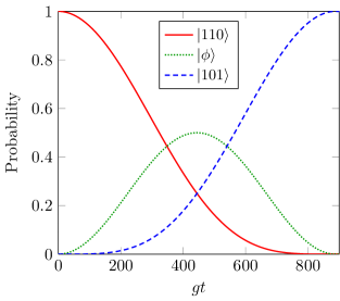
Figure 4: [Color online] The Fredkin gate using the three-state model of Eqs. (16) for parameters in the Hamiltonian (8). The coupling constants $g_{\mathrm{ab}}$ to $g_{\mathrm{fa}}$ are set to $g$ and $\Delta_{1}$, $\Delta_{2}$, $\Delta_{4}$ and $\Delta_{5}$ are all set to 20$g$ so that $g_{1}=g_{2}$. The detunings $\Delta_{3}$ and $\Delta_{6}$ are set by the resonance conditions (16). This plot shows populations of the three states of the system which oscillate to produce the gate evolution [approximately given by Eq. (18)]. Other states that represent qubits will remain essentially unchanged.

We have tested this theory by numerically integrating the full Hamiltonian (8) and checking that the appropriate gate operation takes place. Figure 4 shows the population of three of the states corresponding to those in Eq. (18) with good population swapping. The fidelity of the exact numerical dynamics to the analytic behavior in Eq. (18) is shown in Fig. 5 (solid line). We note that the fidelity can be enhanced (dashed line) by measuring the atom state to be $\left|a\right\rangle$. This forms a simple error correction or state locking. If the atom is not found to be in state $\left|a\right\rangle$, the logic operation must be aborted.

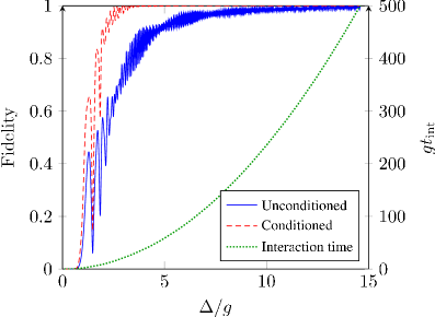
Figure 5: [Color online] Left axis: Fidelity of the Fredkin gate (solid line) as a function of a detuning $\Delta=\Delta_{i}$, for $i=1,2,4,5$. The detunings $\Delta_{3}$ and $\Delta_{6}$ are determined by Eqs. (16) with couplings $g_{i}^{\alpha\beta}=g$. The dashed line shows the improvement resulting from a conditional measurement on the atom after it has left the cavity. Right axis: The dotted line shows the interaction time $t_{\mathrm{int}}=\pi/g^{\prime}$ as found from the three-state model (18).

V Qubit rotations

In addition to the Fredkin gate, an entangling multi-qubit gate, we also need to be able to rotate an individual qubit over the Bloch-sphere to complete a universal set of gates. Rotations in any two of $x$, $y$ and $z$ are capable, in combination, of producing an arbitrary rotation, so it is sufficient to show that two of these rotations are possible using the system detailed above. The Jaynes-Cummings model with a large detuning realizes a simple rotation about $z$ ($\hat{R}_{z}$) with a two-level atom detuned from the first mode of a qubit, and far detuned from the other mode. With the qubit represented as in Table 1, we will have $\left|1\right\rangle\rightarrow\mathrm{e}^{i(g^{2}/\Delta)t}\left|1\right\rangle$ while $\left|0\right\rangle\rightarrow\left|0\right\rangle$ at time $t$. If the cavity field varies spatially, one can simply adjust the interaction time to compensate Englert et al. (1998).

To complete the set of gates we can form an $x$-rotation using a lambda scheme with the two transitions coupled to the two modes that make up a qubit as shown in Fig. 6.

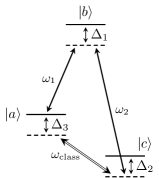
Figure 6: The lambda atom has two transitions which couple to the two cavity modes that make up a qubit. We adiabatically eliminate levels $\left|b\right\rangle$ and $\left|c\right\rangle$ from the interaction under the conditions (20).

A strong classical field couples the ground states together with coupling $\Omega/2$ and the gate is formed when the qubit modes are detuned and a loop resonance exists. Under the conditions

$$\Delta_{1},\,\Delta_{2}\gg g^{\mathrm{ab}}_{1},\,g^{\mathrm{bc}}_{2},\,\Omega/2,\,\Delta_{3}$$ (20)

we again have an effective two-level system with the atom in state $\left|a\right\rangle$ in both “levels.” The resonance condition is (see Appendix C)

$$\Delta_{\mathrm{eff}}=\Delta_{3}+\frac{(g^{\mathrm{ab}}_{1})^{2}}{\Delta_{1}}$$ (21)

which can be controlled via several free parameters. Similarly, the effective coupling constant is

$$g_{\mathrm{eff}}=-\frac{g^{\mathrm{ab}}_{1}g^{\mathrm{bc}}_{2}\Omega}{2\Delta_{1}\Delta_{2}},$$ (22)

so that, finally, the $x$-rotation operation becomes $\hat{R}_{x}(t)=\cos(g_{\mathrm{eff}}t)\hat{I}-i\sin(g_{\mathrm{eff}}t)\hat{\sigma}_{x}$.

VI Conclusion

In summary, we have seen that multi-photon resonances in cavities can realize a universal set of logic gates. The multiphoton resonances are possible because of the strong single-photon couplings (and long decay times) available in high-$Q$ cavities. We can locate the resonances by utilizing effective Hamiltonians for the combined atom-field states. For realizable microwave cavities, we find a Fredkin gate operation time of $4\times 10^{-4}$ s for $\Delta\sim 5g$, which is well within a photon lifetime of $\sim 0.3$ s. Results on the more quantitative effects of decoherence are discussed in Ref. Alqahtani et al. (2014). If we make a measurement-based selection of the atom leaving the cavity, the fidelity is $\sim 1-6\times 10^{-4}$ (at $\Delta\sim 5g$ in Fig. 5), falling to $\sim 0.91$ if no measurement is made. Some tuning of the energy levels may be achieved by Stark shifting the Rydberg states Larson and Garraway (2004).

The system is reasonably insensitive to variations in parameters (Fig. 5). A Fredkin gate based on resonance, i.e. with all the $\Delta_{i}=0$ (Fig. 3), would be very sensitive and require specific coupling constants Cook and Shore (1979). By allowing resonance in just a few places, i.e. with $\Delta_{3}$ and $\Delta_{6}$, we have reached a practical compromise on sensitivity and gate speed.

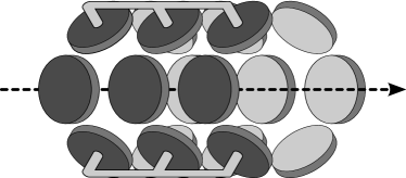
Figure 7: Conceptual, and simplified, illustration of cascaded clusters of six cavities resulting in a scalable system. The path of the ancilla atom is indicated with the arrow. Not shown are the electrodes to be used locally to Stark shift atomic levels out of resonance with the cavity modes as required for the implemented gates.

The system appears to be scalable, though in this paper we have focused on basic logic gates. Of course, scalability is a crucial issue for building a QIP architecture and we indicate some ways in which this can be done. Figure 7 shows the path of an atom through a cascade of cavity clusters, each involving six modes. In this case, depending on whether the levels are in the configuration of Fig. 3, or Fig. 6, we can have different gates operating between the photonic qubits. We recall that in each cluster the atom acts only as an ancilla to bring about the operation. To facilitate communication between cavity clusters, one pair of modes could form a bus mode, if oriented along the axis of travel of the atom. Such a mode pair could interact with any of the cavity clusters as the ancilla atom passes through. Alternatively, the qubit state could be temporarily transferred to the atom to allow inter-cluster communication (though in such a case atoms would have to fly through the cavities in both directions to ensure a two-way flow of information). In all cases, a simple local Stark detuning could be used to “turn off” a cluster, i.e. to prevent its interaction with the ancilla, or bus-mode. Through all these methods, we believe that more complex gates could be built up. However, the multi-photon cavity resonances at the heart of the gates appear to be in the range of practicality. They have not been observed to date and may be an interesting phenomena in themselves with other applications such as the creation of entangled states in cavity resonators.

We thank the UK EPSRC, the Leverhulme Trust and the Japanese Society for the Promotion of Science for their support. Special thanks to Moteb M Alqahtani for comments on the manuscript and to B. Shore.

Appendix A Derivation of the iswap Gate Effective Hamiltonian

A.1 Transformation

The Hamiltonian that describes the level scheme in Fig. 2 in the Schrödinger picture is

$$H=\sum_{\alpha}E_{\alpha}\hat{\sigma}_{\mathrm{\alpha\alpha}}+\sum_{i=1}^{4}\omega_{i}\hat{a}^{\dagger}_{i}\hat{a}_{i}+\left[g^{\mathrm{ab}}_{1}\hat{\sigma}_{\mathrm{ba}}\hat{a}_{1}+g^{\mathrm{bc}}_{2}\hat{\sigma}_{\mathrm{cb}}\hat{a}^{\dagger}_{2}\right.\\ \left.+g^{\mathrm{cd}}_{3}\hat{\sigma}_{\mathrm{dc}}\hat{a}_{3}+g^{\mathrm{da}}_{4}\hat{\sigma}_{\mathrm{ad}}\hat{a}^{\dagger}_{4}+\mathrm{h.c.}\right]\,,$$ (23)

where $\alpha$ represents the energy levels of the atom and $i$ the modes of the field. A transformation operator $T=\exp(i\hat{\Theta}t)$ is defined to move to an interaction picture and remove absolute energy dependence. The new Hamiltonian is given by

$$H^{\prime}=\hat{T}H\hat{T}^{\dagger}-\hat{\Theta}$$ (24)

The choice of the operator $\Theta$ is made to remove the non-interacting terms in the Hamiltonian without introducing time dependence. That is, we let

$$\Theta=\sum_{\alpha}E_{\alpha}\hat{\sigma}_{\mathrm{\alpha\alpha}}+\sum_{i=1}^{4}\hat{a}^{\dagger}_{i}\hat{a}_{i}(\omega_{i}+\delta_{i})\,,$$ (25)

where the $\delta_{i}$ are related to the $\Delta_{j}$ in the level diagram Fig. 2 by

$$\begin{split}\Delta_{1}&=\delta_{1}\\ \Delta_{2}&=\delta_{1}-\delta_{2}\\ \Delta_{3}&=\delta_{1}-\delta_{2}+\delta_{3}\\ \Delta_{4}&=\delta_{1}-\delta_{2}+\delta_{3}-\delta_{4}\,,\end{split}$$ (26)

and $\delta_{i}$ are interpreted as the detuning between a pair of levels and a field mode, whereas $\Delta_{j}$ are the detunings of levels from level $\left|a\right\rangle$ and a multi-photon transition. This transformation yields the Hamiltonian

$$H=-\sum_{i=1}^{4}\delta_{i}\hat{a}^{\dagger}_{i}\hat{a}_{i}+\left[g^{\mathrm{ab}}_{1}\hat{\sigma}_{\mathrm{ba}}\hat{a}_{1}+g^{\mathrm{bc}}_{2}\hat{\sigma}_{\mathrm{cb}}\hat{a}^{\dagger}_{2}\right.\\ \left.+g^{\mathrm{cd}}_{3}\hat{\sigma}_{\mathrm{dc}}\hat{a}_{3}+g^{\mathrm{da}}_{4}\hat{\sigma}_{\mathrm{ad}}\hat{a}^{\dagger}_{4}+\mathrm{h.c.}\right]\,,$$ (27)

which leads us to Eq. (3) on utilizing Eq. (26) for the $\delta_{i}$.

A.2 The Effective Hamiltonian

We follow a procedure from a paper by Shore Shore (1981). We define two projection operators, $\hat{P}$ and $\hat{Q}$, to select out the states close to resonance and far from resonance, respectively. In this assumption $\Delta_{i}\gg g^{\mathrm{\alpha\beta}}_{j}$ where $g^{\mathrm{\alpha\beta}}_{j}$ represents all of the coupling constants and $i=1,2,3,4$. $\Delta_{4}$ will be small and chosen later to ensure resonance. From this we define the components $H_{0}=\hat{P}H\hat{P}^{\dagger}$, $\hat{B}=\hat{P}H\hat{Q}^{\dagger}$ and $A=\hat{Q}H\hat{Q}^{\dagger}$. For systems with a small Hilbert space it is simplest to proceed in matrix form. If the system is initially in one of the states $\left|1010,a\right\rangle$ or $\left|0101,a\right\rangle$ then at some time later the state of the system will be $\left|\Psi\right\rangle=c_{1}\left|1010,a\right\rangle+c_{2}\left|0010,b\right\rangle+c_{3}\left|0110,c\right\rangle+c_{4}\left|0100,d\right\rangle+c_{5}\left|0101,a\right\rangle$. The Hamiltonian in matrix form is

$$H=\begin{pmatrix}0&g^{\mathrm{ab}}_{1}&0&0&0\\ g^{\mathrm{ab}}_{1}&\Delta_{1}&g^{\mathrm{bc}}_{2}&0&0\\ 0&g^{\mathrm{bc}}_{2}&\Delta_{2}&g^{\mathrm{cd}}_{3}&0\\ 0&0&g^{\mathrm{cd}}_{3}&\Delta_{3}&g^{\mathrm{da}}_{4}\\ 0&0&0&g^{\mathrm{da}}_{4}&\Delta_{4}\end{pmatrix}\,, \left|\Psi\right\rangle=\begin{pmatrix}c_{1}\\ c_{2}\\ c_{3}\\ c_{4}\\ c_{5}\end{pmatrix}\,.$$ (28)

The operators $H_{0}$, $\hat{A}$ and $\hat{B}$ can be found by manipulating the Hamiltonian matrix so that the two states close to resonance are put to the top of the state vector.

$$H=\begin{pmatrix}0&0&g^{\mathrm{ab}}_{1}&0&0\\ 0&\Delta_{4}&0&0&g^{\mathrm{da}}_{4}\\ g^{\mathrm{ab}}_{1}&0&\Delta_{1}&g^{\mathrm{bc}}_{2}&0\\ 0&0&g^{\mathrm{bc}}_{2}&\Delta_{2}&g^{\mathrm{cd}}_{3}\\ 0&g^{\mathrm{da}}_{4}&0&g^{\mathrm{cd}}_{3}&\Delta_{3}\end{pmatrix}\,, \left|\Psi\right\rangle=\begin{pmatrix}c_{1}\\ c_{5}\\ c_{2}\\ c_{3}\\ c_{4}\end{pmatrix}\,.$$ (29)

When this has been done the Hamiltonian is broken into the parts.

$$H_{0}=\begin{pmatrix}0&0\\ 0&\Delta_{4}\end{pmatrix}\,, A=\begin{pmatrix}\Delta_{1}&g^{\mathrm{bc}}_{2}&0\\ g^{\mathrm{bc}}_{2}&\Delta_{2}&g^{\mathrm{cd}}_{3}\\ 0&g^{\mathrm{cd}}_{3}&\Delta_{3}\end{pmatrix}\,,$$ (30)

$$B=\begin{pmatrix}g^{\mathrm{ab}}_{1}&0&0\\ 0&0&g^{\mathrm{da}}_{4}\end{pmatrix}\,.$$

Using these parts the effective Hamiltonian is constructed according to the equation Shore (1981)

$$H_{\mathrm{eff}}=H_{0}-BA^{-1}B^{\dagger}\,,$$ (31)

which, after a trivial energy shift, results in the two-state effective Hamiltonian

$$H_{\mathrm{eff}}=\begin{pmatrix}0&g_{\mathrm{eff}}\\ g_{\mathrm{eff}}&\Delta_{\mathrm{eff}}\end{pmatrix}\,,$$ (32)

where

$$\begin{split}g_{\mathrm{eff}}&=-\frac{g^{\mathrm{ab}}_{1}g^{\mathrm{bc}}_{2}g^{\mathrm{cd}}_{3}g^{\mathrm{da}}_{4}}{\Delta_{1}\Delta_{2}\Delta_{3}-\Delta_{3}(g^{\mathrm{bc}}_{2})^{2}-\Delta_{1}(g^{\mathrm{cd}}_{3})^{2}}\\ &\approx-\frac{g^{\mathrm{ab}}_{1}g^{\mathrm{bc}}_{2}g^{\mathrm{cd}}_{3}g^{\mathrm{da}}_{4}}{\Delta_{1}\Delta_{2}\Delta_{3}}\,,\end{split}$$ (33)

and

$$\begin{split}&\Delta_{\mathrm{eff}}=\\ &\Delta_{4}+\frac{(g^{\mathrm{ab}}_{1})^{2}(\Delta_{2}\Delta_{3}-(g^{\mathrm{cd}}_{3})^{2})-(g^{\mathrm{da}}_{4})^{2}(\Delta_{1}\Delta_{2}-(g^{\mathrm{bc}}_{2})^{2})}{\Delta_{1}\Delta_{2}\Delta_{3}-\Delta_{3}(g^{\mathrm{bc}}_{2})^{2}-\Delta_{1}(g^{\mathrm{cd}}_{3})^{2}}\\ &\approx\Delta_{4}+\frac{(g^{\mathrm{ab}}_{1})^{2}}{\Delta_{1}}-\frac{(g^{\mathrm{da}}_{4})^{2}}{\Delta_{3}}\,,\end{split}$$ (34)

which are the results given in Section III.

Appendix B Derivation of the Fredkin Gate Effective Hamiltonian

B.1 Transformations

The Hamiltonian that describes the level scheme in Fig. 3 is

$$\begin{split}H=&\sum_{\alpha}E_{\alpha}\hat{\sigma}_{\mathrm{\alpha\alpha}}+\sum_{i\neq 4}\omega_{i}\hat{a}^{\dagger}_{i}\hat{a}_{i}\\ &+\left[g^{\mathrm{ab}}_{1}\hat{\sigma}_{\mathrm{ba}}\hat{a}_{1}+g^{\mathrm{bc}}_{2}\hat{\sigma}_{\mathrm{cb}}\hat{a}^{\dagger}_{2}+g^{\mathrm{cd}}_{3}\hat{\sigma}_{\mathrm{dc}}\hat{a}_{3}\right.\\ &\left.+g^{\mathrm{de}}_{1}\hat{\sigma}_{\mathrm{ed}}\hat{a}^{\dagger}_{1}+g^{\mathrm{ef}}_{5}\hat{\sigma}_{\mathrm{fe}}\hat{a}_{5}+g^{\mathrm{af}}_{6}\hat{\sigma}_{\mathrm{af}}\hat{a}^{\dagger}_{6}+\mathrm{h.c.}\right]\,,\end{split}$$ (35)

where we note the repeated mode 1 in the interaction terms and the absence of mode 4 so that for the sum over $i$ we have $i=1,2,3,5,6$. To proceed to an interaction picture, we define a transformation through $\hat{T_{1}}=\exp(i\hat{\Theta}_{1}t)$ which will modify the Hamiltonian according to (24). The full transformation will be made in two steps. For the first step in the transformation we remove explicit dependence on the atomic energy levels

$$\hat{\Theta}_{1}=\sum_{\alpha}E_{\alpha}\hat{\sigma}_{\mathrm{\alpha\alpha}}+\sum_{i\neq 4}\hat{a}^{\dagger}_{i}\hat{a}_{i}(\omega_{i}+\delta_{i})$$ (36)

where $\delta_{i}$ are the detunings between particular atomic transitions and the relevant mode, i.e. $E_{\mathrm{d}}-E_{\mathrm{c}}=\omega_{3}+\delta_{3}$. Figure 8 shows how these relate to the $\Delta_{i}$ in Figure 3.

Figure 8: This diagram illustrates the difference between the detunings $\Delta_{i}$ in Figure 3 and the detunings $\delta_{i}$ utilized in Appendix B. The detunings $\delta_{i}$ indicate the detuning of each coupled field from its respective transition. The detunings $\Delta_{i}$ represent the accumulated detuning of a multi-photon resonance (without considering level shifts).

Specifically

$$\begin{split}\Delta_{1}&=\delta_{1}\\ \Delta_{2}&=\delta_{1}-\delta_{2}\\ \Delta_{3}&=\delta_{1}-\delta_{2}+\delta_{3}\\ \Delta_{4}&=\delta_{1}-\delta_{2}+\delta_{3}-\delta_{4}\\ \Delta_{5}&=\delta_{1}-\delta_{2}+\delta_{3}-\delta_{4}+\delta_{5}\\ \Delta_{6}&=\delta_{1}-\delta_{2}+\delta_{3}-\delta_{4}+\delta_{5}-\delta_{6}\,.\end{split}$$ (37)

Note that there is no provision for $\delta_{4}$ in the transformation with $\hat{\Theta}_{1}$, Eq. (36), as mode four is not present. (It is replaced by mode 1.) This choice for $\hat{\Theta}_{1}$ avoids time dependence in most elements in the resultant Hamiltonian

$$H^{\prime}=-\sum_{i\neq 4}\delta_{i}\hat{a}^{\dagger}_{i}\hat{a}_{i}+\left[g^{\mathrm{ab}}_{1}\hat{\sigma}_{\mathrm{ba}}\hat{a}_{1}+g^{\mathrm{bc}}_{2}\hat{\sigma}_{\mathrm{cb}}\hat{a}^{\dagger}_{2}+g^{\mathrm{cd}}_{3}\hat{\sigma}_{\mathrm{dc}}\hat{a}_{3}\right.\\ \left.+g^{\mathrm{de}}_{1}\mathrm{e}^{i(\delta_{1}-\delta_{4})t}\hat{\sigma}_{\mathrm{ed}}\hat{a}^{\dagger}_{1}+g^{\mathrm{ef}}_{5}\hat{\sigma}_{\mathrm{fe}}\hat{a}_{5}+g^{\mathrm{af}}_{6}\hat{\sigma}_{\mathrm{af}}\hat{a}^{\dagger}_{6}+\mathrm{h.c.}\right]\,.$$ (38)

We make a second transformation to remove some remaining time dependence

$$\hat{\Theta}_{2}=\left(\hat{n}_{1}+\hat{n}_{2}+\hat{n}_{3}+\hat{n}_{6}-\hat{\sigma}_{\mathrm{aa}}-\hat{\sigma}_{\mathrm{cc}}\right)(\delta_{4}-\delta_{1})\,.$$ (39)

The resultant Hamiltonian is

$$H^{\prime\prime}=-\sum_{i\neq 4}\delta_{i}\hat{a}^{\dagger}_{i}\hat{a}_{i}+\left[g^{\mathrm{ab}}_{1}\hat{\sigma}_{\mathrm{ba}}\hat{a}_{1}+g^{\mathrm{bc}}_{2}\hat{\sigma}_{\mathrm{cb}}\hat{a}^{\dagger}_{2}+g^{\mathrm{cd}}_{3}\hat{\sigma}_{\mathrm{dc}}\hat{a}_{3}\right.\\ \left.+g^{\mathrm{de}}_{1}\hat{\sigma}_{\mathrm{ed}}\hat{a}^{\dagger}_{1}+g^{\mathrm{ef}}_{5}\hat{\sigma}_{\mathrm{fe}}\hat{a}_{5}+g^{\mathrm{af}}_{6}\hat{\sigma}_{\mathrm{af}}\hat{a}^{\dagger}_{6}+\mathrm{h.c.}\right]-\hat{\Theta}_{2}\,.$$ (40)

When we express $H^{\prime\prime}$ in terms of $\Delta_{i}$, Eq. (8) is recovered.

B.2 Effective 2-State Behavior

Following the procedure outlined in Appendix A.2 Shore (1981) we define two projection operators, $\hat{P}$ and $\hat{Q}$, to select out the states close to resonance and far from resonance respectively. In this assumption $\Delta_{i}\gg g^{\mathrm{\alpha\beta}}_{j}$ where $g^{\mathrm{\alpha\beta}}_{j}$ represents all of the coupling constants and $i=1,2,3,4,5$. $\Delta_{6}$ will be small and is chosen later to ensure resonance. As before, we define the components $H_{0}=\hat{P}H\hat{P}^{\dagger}$, $\hat{B}=\hat{P}H\hat{Q}^{\dagger}$ and $A=\hat{Q}H\hat{Q}^{\dagger}$. Given these new operators the effective Hamiltonian is defined as

$$H_{\mathrm{eff}}=H_{0}-\hat{B}\hat{A}^{-1}\hat{B}^{\dagger}\,$$ (41)

as in Eq. (31). The operator $\hat{P}$ projects onto states of the system we expect to be populated, $\left|10,01,10,a\right\rangle$ and $\left|10,10,01,a\right\rangle$. The operator $\hat{Q}$ projects onto the states that we expect to be suppressed: $\left|00,01,10,b\right\rangle$, $\left|00,11,10,c\right\rangle$, $\left|00,10,10,d\right\rangle$, $\left|10,10,10,e\right\rangle$, $\left|10,10,00,f\right\rangle$, $\left|00,10,01,b\right\rangle$ and $\left|01,10,01,c\right\rangle$, with this order chosen such that the matrix $A$ is tridiagonal. As the system has a small Hilbert space, the resultant operators are best shown as matrices. Note that an additional trivial transformation has been made to set the energy of the state $\left|10,01,10,a\right\rangle$ (see Eq. (9)) to zero as a reference point. Then

$$H_{0}=\begin{pmatrix}0&0\\ 0&\Delta_{6}\end{pmatrix}\,,\ B=\begin{pmatrix}g^{\mathrm{ab}}_{1}&0&0&0&0&0&0\\ 0&0&0&0&g^{\mathrm{fa}}_{6}&g^{\mathrm{ab}}_{1}&0\end{pmatrix}\,,$$ (42)

and $A$ is a $7\times 7$ matrix composed of the detuned portion of the Hamiltonian

$$A=\begin{pmatrix}\Delta_{1}&g^{\mathrm{bc}}_{2}&0&0&0&0&0\\ g^{\mathrm{bc}}_{2}&\Delta_{2}&g^{\mathrm{cd}}_{3}&0&0&0&0\\ 0&g^{\mathrm{cd}}_{3}&\Delta_{3}&g^{\mathrm{de}}_{1}&0&0&0\\ 0&0&g^{\mathrm{de}}_{1}&\Delta_{4}&g^{\mathrm{ef}}_{5}&0&0\\ 0&0&0&g^{\mathrm{ef}}_{5}&\Delta_{5}&0&0\\ 0&0&0&0&0&\Delta_{6}+\Delta_{1}&g^{\mathrm{bc}}_{2}\sqrt{2}\\ 0&0&0&0&0&g^{\mathrm{bc}}_{2}\sqrt{2}&\Delta_{6}+\Delta_{1}\end{pmatrix}\,.$$ (43)

The matrix $A$ must be inverted, but as B has two populated elements, only four elements of $A^{-1}$ need be calculated for use in equation (41). The resultant two state effective Hamiltonian produced using equation (41) is

$$H_{\mathrm{eff}}=\begin{pmatrix}0&g_{\mathrm{eff}}\\ g_{\mathrm{eff}}&\Delta_{\mathrm{eff}}\end{pmatrix}\,,$$ (44)

where

$$\begin{split}g_{\mathrm{eff}}&\approx-\frac{g^{\mathrm{ab}}_{1}g^{\mathrm{bc}}_{2}g^{\mathrm{cd}}_{3}g^{\mathrm{de}}_{1}g^{\mathrm{ef}}_{5}g^{\mathrm{fa}}_{6}}{\Delta_{1}\Delta_{2}\Delta_{3}\Delta_{4}\Delta_{5}}\,,\\ \Delta_{\mathrm{eff}}&\approx\Delta_{6}-\frac{(g^{\mathrm{fa}}_{6})^{2}}{\Delta_{5}}\,.\end{split}$$ (45)

Note that (45) may appear to be missing a term when compared with (34). This is due to the lower right $2\times 2$ submatrix in (43), which deals with a mode with two excitations. This is not present in the iswap gate, and to first order leads to one less term in (45).

B.3 Effective 3-State Behavior

To produce an effective three level system with the states $\left|10,01,10,a\right\rangle$, $\left|00,10,10,d\right\rangle$ and $\left|10,10,01,a\right\rangle$ we generalize the procedure in Appendix B.2. We use the same full set of states $\left|10,01,10,a\right\rangle$, $\left|00,01,10,b\right\rangle$, $\left|00,11,10,c\right\rangle$, $\left|00,10,10,d\right\rangle$, $\left|10,10,10,e\right\rangle$, $\left|10,10,00,f\right\rangle$, $\left|10,10,01,a\right\rangle$, $\left|00,10,01,b\right\rangle$ and $\left|01,10,01,c\right\rangle$, allowing the state $\left|00,10,10,d\right\rangle$ to be close to resonance in addition to $\left|10,01,10,a\right\rangle$ and $\left|10,10,01,a\right\rangle$. The detuning $\Delta_{3}$ is chosen later to ensure resonance. The resultant operators are

$$H_{0}=\begin{pmatrix}0&0&0\\ 0&\Delta_{3}&0\\ 0&0&\Delta_{6}\end{pmatrix},\ B=\begin{pmatrix}g^{\mathrm{ab}}_{1}&0&0&0&0&0\\ 0&g^{\mathrm{cd}}_{3}&g^{\mathrm{de}}_{1}&0&0&0\\ 0&0&0&g^{\mathrm{af}}_{6}&g^{\mathrm{ab}}_{1}&0\end{pmatrix},$$ (46)

and $A$ is the $6\times 6$ matrix composed of the detuned portion of the Hamiltonian

$$A=\begin{pmatrix}\Delta_{1}&g^{\mathrm{bc}}_{2}&0&0&0&0\\ g^{\mathrm{bc}}_{2}&\Delta_{2}&0&0&0&0\\ 0&0&\Delta_{4}&g^{\mathrm{ef}}_{5}&0&0\\ 0&0&g^{\mathrm{ef}}_{5}&\Delta_{5}&0&0\\ 0&0&0&0&\Delta_{6}+\Delta_{1}&g^{\mathrm{bc}}_{2}\sqrt{2}\\ 0&0&0&0&g^{\mathrm{bc}}_{2}\sqrt{2}&\Delta_{6}+\Delta_{2}\end{pmatrix}\,.$$ (47)

The subsystem associated with $H_{0}$ is composed of the states $\left|10,01,10,a\right\rangle$, $\left|00,10,10,d\right\rangle$ and $\left|10,10,01,a\right\rangle$. Then by utilizing Eq. (41), the full matrix for the effective Hamiltonian is

$$H_{\mathrm{eff}}=\begin{pmatrix}0&g_{1}&0\\ g_{1}&\Delta_{1}^{\mathrm{eff}}&g_{2}\\ 0&g_{2}&\Delta_{2}^{\mathrm{eff}}\end{pmatrix}\,,$$ (48)

where

$$g_{1} =\frac{g^{\mathrm{ab}}_{1}g^{\mathrm{bc}}_{2}g^{\mathrm{cd}}_{3}}{\Delta_{1}\Delta_{2}}, g_{2} =\frac{g^{\mathrm{de}}_{1}g^{\mathrm{ef}}_{5}g^{\mathrm{fa}}_{6}}{\Delta_{4}\Delta_{5}}\,,$$ (49)

and

$$\begin{split}&\Delta_{1}^{\mathrm{eff}}\approx\Delta_{3}+\frac{\left(g^{\mathrm{ab}}_{1}\right)^{2}}{\Delta_{1}}-\frac{\left(g^{\mathrm{cd}}_{3}\right)^{2}}{\Delta_{2}}-\frac{\left(g^{\mathrm{de}}_{1}\right)^{2}}{\Delta_{4}}\,,\\ &\Delta_{2}^{\mathrm{eff}}\approx\Delta_{6}-\frac{\left(g^{\mathrm{af}}_{6}\right)^{2}}{\Delta_{5}}\,.\end{split}$$ (50)

The conditions for the fast Fredkin gate (16), (17) and (18) are derived from the Hamiltonian in (48). For the gate to operate, the second and third diagonal elements must be equal to the first.

Appendix C Derivation of the $x$-Rotation Gate

The Hamiltonian that describes the system shown in Fig. 6 is

$$\begin{split}H=&E_{\mathrm{a}}\hat{\sigma}_{\mathrm{aa}}+E_{\mathrm{b}}\hat{\sigma}_{\mathrm{bb}}+E_{\mathrm{c}}\hat{\sigma}_{\mathrm{cc}}+\omega_{1}\hat{a}^{\dagger}_{1}\hat{a}_{1}+\omega_{2}\hat{a}^{\dagger}_{2}\hat{a}_{2}\\ &+\left[g^{\mathrm{ab}}_{1}\hat{a}^{\dagger}_{1}\hat{\sigma}_{\mathrm{ab}}+g^{\mathrm{bc}}_{2}\hat{a}^{\dagger}_{2}\hat{\sigma}_{\mathrm{cb}}+\frac{\Omega}{2}\mathrm{e}^{i\omega_{3}t}\hat{\sigma}_{\mathrm{ca}}+\mathrm{h.c.}\right]\,.\end{split}$$ (51)

As with the derivation of the Fredkin gate, the detuning is defined for each transition such that

$$\begin{split}E_{\mathrm{b}}-E_{\mathrm{a}}&=\omega_{1}+\delta_{1}\\ E_{\mathrm{b}}-E_{\mathrm{c}}&=\omega_{2}+\delta_{2}\\ E_{\mathrm{a}}-E_{\mathrm{c}}&=\omega_{3}+\delta_{3}\end{split}$$ (52)

and the link between $\Delta_{i}$ and $\delta_{i}$ is

$$\begin{split}\Delta_{1}&=\delta_{1}\\ \Delta_{2}&=\delta_{1}-\delta_{2}\\ \Delta_{3}&=\delta_{1}-\delta_{2}+\delta_{3}\,.\end{split}$$ (53)

As in Appendix B.1 a transformation operator is chosen

$$\hat{T}=\exp\left(i\hat{\Theta}_{1}t\right)\,,$$ (54)

where

$$\hat{\Theta}_{1}=\sum_{\alpha=\mathrm{a},\mathrm{b},\mathrm{c}}E_{\alpha}\hat{\sigma}_{\mathrm{\alpha\alpha}}+\sum_{i=1,2}\hat{a}^{\dagger}_{i}\hat{a}_{i}\left(\omega_{i}+\delta_{i}\right)\,.$$ (55)

After the transformation the Hamiltonian is

$$\begin{split}H^{\prime}=&-\delta_{1}\hat{a}^{\dagger}_{1}\hat{a}_{1}-\delta_{2}\hat{a}^{\dagger}_{2}\hat{a}_{2}\\ &+\left[g^{\mathrm{ab}}_{1}\hat{a}^{\dagger}_{1}\hat{\sigma}_{\mathrm{ab}}+g^{\mathrm{bc}}_{2}\hat{a}^{\dagger}_{2}\hat{\sigma}_{\mathrm{cb}}+\frac{\Omega}{2}\mathrm{e}^{-i\delta_{3}t}\hat{\sigma}_{\mathrm{ca}}+\mathrm{h.c.}\right].\end{split}$$ (56)

A second transformation is made to remove the remaining time dependence

$$\hat{\Theta}_{2}=\frac{1}{2}\left(\hat{a}^{\dagger}_{1}\hat{a}_{1}-\hat{a}^{\dagger}_{2}\hat{a}_{2}+\hat{\sigma}_{\mathrm{cc}}-\hat{\sigma}_{\mathrm{aa}}\right)\delta_{3}-\delta_{1}\,.$$ (57)

The Hamiltonian is now

$$\begin{split}H^{\prime\prime}=&-\delta_{1}\hat{a}^{\dagger}_{1}\hat{a}_{1}-\delta_{2}\hat{a}^{\dagger}_{2}\hat{a}_{2}-\hat{\Theta}_{2}\\ &+\left[g^{\mathrm{ab}}_{1}\hat{a}^{\dagger}_{1}\hat{\sigma}_{\mathrm{ab}}+g^{\mathrm{bc}}_{2}\hat{a}^{\dagger}_{2}\hat{\sigma}_{\mathrm{cb}}+\frac{\Omega}{2}\hat{\sigma}_{\mathrm{ca}}+\mathrm{h.c.}\right].\end{split}$$ (58)

Assuming that only one excitation exists in the system, the wavefunction is

$$\left|\Psi\right\rangle=c_{0}\left|1,0,c\right\rangle+c_{1}\left|1,0,a\right\rangle\\ +c_{2}\left|0,0,b\right\rangle+c_{3}\left|0,1,c\right\rangle+c_{4}\left|0,1,a\right\rangle\,.$$ (59)

The procedure for producing an effective Hamiltonian is now followed exactly as in Ref. Shore (1981) for atomic states alone. The Hamiltonian, under the assumption of only one excitation, can be displayed as the matrix

$$H^{\prime\prime}=\begin{pmatrix}\Delta_{2}-\Delta_{3}&\Omega/2&0&0&0\\ \Omega/2&0&g^{\mathrm{ab}}_{1}&0&0\\ 0&g^{\mathrm{ab}}_{1}&\Delta_{1}&g^{\mathrm{bc}}_{2}&0\\ 0&0&g^{\mathrm{bc}}_{2}&\Delta_{2}&\Omega/2\\ 0&0&0&\Omega/2&\Delta_{3}\end{pmatrix}, \left|\Psi\right\rangle=\begin{pmatrix}c_{0}\\ c_{1}\\ c_{2}\\ c_{3}\\ c_{4}\end{pmatrix}.$$ (60)

The matrix is rearranged to place the two states of the system that are close to resonance to the top of the state vector. We consider the case when the atom is initially in the state $\left|a\right\rangle$, so both states of the system with the atom state as $\left|a\right\rangle$ are close to resonance. In other words, $g^{\mathrm{ab}}_{1},g^{\mathrm{bc}}_{2},\Omega/2,\Delta_{3}\ll\Delta_{1},\Delta_{2}$.

$$H^{\prime\prime}=\begin{pmatrix}0&0&g^{\mathrm{ab}}_{1}&0&\Omega/2\\ 0&\Delta_{3}&0&\Omega/2&0\\ g^{\mathrm{ab}}_{1}&0&\Delta_{1}&g^{\mathrm{bc}}_{2}&0\\ 0&\Omega/2&g^{\mathrm{ab}}_{2}&\Delta_{2}&0\\ \Omega/2&0&0&0&\Delta_{2}-\Delta_{3}\end{pmatrix}, \left|\Psi\right\rangle=\begin{pmatrix}c_{1}\\ c_{4}\\ c_{2}\\ c_{3}\\ c_{0}\end{pmatrix}.$$ (61)

The top left $2\times 2$ matrix is $H_{0}$, the bottom right $3\times 3$ is $A$, and the top right partition is $B$:

$$H_{0}=\begin{pmatrix}0&0\\ 0&\Delta_{3}\end{pmatrix}\,, A=\begin{pmatrix}\Delta_{1}&g^{\mathrm{bc}}_{2}&0\\ g^{\mathrm{bc}}_{2}&\Delta_{2}&0\\ 0&0&\Delta_{2}-\Delta_{3}\end{pmatrix}\,,$$ (62)

$$B=\begin{pmatrix}g^{\mathrm{ab}}_{1}&0&\Omega/2\\ 0&\Omega/2&0\end{pmatrix}.$$ (63)

The assumption that $g^{\mathrm{ab}}_{1},g^{\mathrm{bc}}_{2},\Omega/2,\Delta_{3}\ll\Delta_{1},\Delta_{2}$ was already made, so using equation (41) the approximate effective Hamiltonian is

$$H_{\mathrm{eff}}\approx\begin{pmatrix}-(g^{\mathrm{ab}}_{1})^{2}/\Delta_{1}-\Omega^{2}/4\Delta_{2}&g^{\mathrm{ab}}_{1}g^{\mathrm{bc}}_{2}\Omega/2\Delta_{1}\Delta_{2}\\ g^{\mathrm{ab}}_{1}g^{\mathrm{bc}}_{2}\Omega/2\Delta_{1}\Delta_{2}&\Delta_{3}-\Omega^{2}/4\Delta_{2}\end{pmatrix}\,.$$ (64)

From this equation the effective detuning is the difference between the diagonal elements (21) and the effective coupling constant is the off-diagonal element (22)

$$\Delta_{\mathrm{eff}}\approx\Delta_{3}+\frac{(g^{\mathrm{ab}}_{1})^{2}}{\Delta_{1}}\,, g_{\mathrm{eff}}\approx\frac{g^{\mathrm{ab}}_{1}g^{\mathrm{bc}}_{2}\Omega}{2\Delta_{1}\Delta_{2}}\,.$$ (65)