Polariton linewidth and the reservoir temperature dynamics in a semiconductor microcavity

Abstract

A method of determining the temperature of the nonradiative reservoir in a microcavity exciton-polariton system is developed. A general relation for the homogeneous polariton linewidth is theoretically derived and experimentally used in the method. In experiments with a GaAs microcavity under nonresonant pulsed excitation, the reservoir temperature dynamics is extracted from the polariton linewidth. Within the first nanosecond the reservoir temperature greatly exceeds the lattice temperature and determines the dynamics of the major processes in the system. It is shown that, for nonresonant pulsed excitation of GaAs microcavities, the polariton Bose-Einstein condensation is typically governed by polariton-phonon scattering, while interparticle scattering leads to condensate depopulation.

I Introduction

Experimental investigation and practical use of semiconductor structures in most cases require their nonresonant excitation. The latter leads to a complex evolution of the electron-hole (e-h) system, and this evolution involves several processes Shah (1999): First, internal thermal equilibrium is established within charge carriers in a time shorter than 1 ps for GaAs-based quantum well (QW) structures (considered further in the present paper) Knox et al. (1986, 1988). When the internal equilibrium has been established, the e-h system is characterized by a temperature $T$ greater than the lattice temperature $T_{\text{latt}}$. Second, the e-h system cools down due to the emission of optical (fast stage) and acoustical (slow stage) phonons Leo et al. (1988a, b); Yoon et al. (1996); Rosenwaks et al. (1993). Both processes are accompanied by the exciton formation. The characteristic time of the exciton formation ranges from 10 ps to 1 ns and is determined by the e-h density (see Szczytko et al. (2004) and references therein). For the excitation above the QW barriers the whole evolution is accompanied by the capture of charge carriers to the QWs. For sufficiently deep QW states the capture is relatively fast, with a time of $\sim 1$ ps, and is assisted by the emission of optical phonons Deveaud et al. (1988); Barros et al. (1993); Oberli et al. (1989); Sotirelis and Hess (1994).

The temperature $T$ of the e-h system during its cooldown remains significantly higher than the lattice temperature $T_{\text{latt}}$ for several hundreds of picoseconds in the low-temperature experiments Yoon et al. (1996); Leo et al. (1988a, b); Szczytko et al. (2004); Hoyer et al. (2005). As a result, the dynamics of $T$ determines the exciton fraction and many important properties of the system. An example is Bose-Einstein condensation (BEC) of excitons, which is hindered in bulk semiconductors and the QWs without spatial separation of electrons and holes. The reason for such a hindrance is insufficiently fast cooling of excitons compared with their recombination and inelastic collisions, the latter leading to the formation of the exciton complexes and e-h liquid Bagaev et al. (2010).

We are interested in the temperature dynamics of the reservoir, the e-h system in the QWs embedded in a semiconductor microcavity (MC), and the effect of this dynamics on the properties of MC exciton polaritons, mixed exciton-photon states. This system attracts considerable attention, especially inspired by the achievement of BEC of polaritons Kasprzak et al. (2006) and a number of intriguing related phenomena, such as quantized vortices, superfluidity, the Josephson effect, etc. (see Sanvitto and Timofeev (2012) for a review). The dynamics of the reservoir internal temperature after a short-pulse nonresonant excitation is of primary importance because it determines the possibility of and conditions for the polariton BEC. Typically, the internal temperature of the e-h system in bare QW structures is extracted from the Boltzmann tail in the photoluminescence (PL) spectra, which originates from the e-h plasma recombination. However, the recombination is rather weak and requires for a reasonable analysis a high e-h density Leo et al. (1988a) and high quality of QWs Szczytko et al. (2004). For the QWs embedded in a MC, the e-h plasma recombination is even more hindered due to the strong spectrum modification induced by the MC. In some works the temperature was extracted by analyzing the lower polariton (LP) population energy distribution Deng et al. (2003); Kasprzak et al. (2006); Deng et al. (2006); Balili et al. (2007); Kasprzak et al. (2008); Levrat et al. (2010); Kammann et al. (2012). However, the temperature so defined is not the reservoir temperature but, rather, characterizes the degree of nonequilibrium of the low-wave-vector part of the polariton system.

In the present paper, we propose and justify a new method of determining the reservoir temperature from the linewidth of the lower polariton states. We theoretically derive and experimentally use a general relation for the LP homogeneous linewidth via the rate of polariton escape, used to find the reservoir temperature, and the mean polariton occupation number. The extracted reservoir temperature in the experiments with nonresonant pulsed excitation of the GaAs MC decays from about $100$ K at a time of $50-100$ ps after the excitation pulse and relaxes to the lattice temperature $T_{\text{latt}}$ in about $1$ ns. The fact that at long times the extracted temperature follows $T_{\text{latt}}$ as $T_{\text{latt}}$ is changed proves the validity of our method. We conclude that at the conditions of the polariton Bose-Einstein condensation in GaAs MC structures the reservoir temperature greatly exceeds the lattice temperature. This leads to increasing the BEC threshold and degrading the coherence properties compared with those for the reservoir in thermal equilibrium with the lattice. Furthermore, as a result of the large reservoir temperature, BEC in GaAs MCs under nonresonant pulsed excitation is typically governed by polariton-phonon scattering, while scattering of polaritons by excitons and free charge carriers leads to depopulation of the condensate.

II Theory

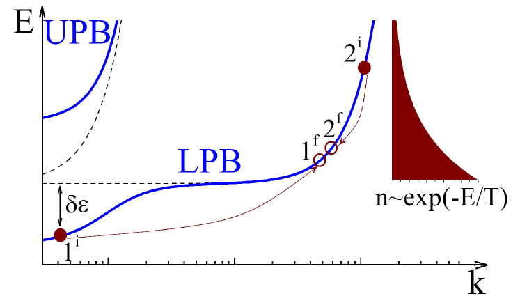
Figure 1: Exciton, photon (dashed lines), and polariton (solid lines) dispersion curves. Arrows show the polariton-exciton scattering responsible for the LP broadening. Filled area shows the reservoir energy distribution (population along the horizontal axis and energy along the vertical axis).

The MC polariton system can be divided into the low-$k$, radiative part ($k$ is a wave vector) and the high-$k$, nonradiative part, usually referred to as a reservoir. In the radiative part, exciton-photon mixing is high, which results in a steep polariton dispersion curve. This polariton part is strongly nonequilibrium due to the short polariton lifetime determined by the MC $Q$ factor. On the other hand, the nonradiative reservoir, containing almost all of the population of the e-h system, is virtually unaffected by the MC, which can only alter the rate of the reservoir density decay induced by exciton scattering to the leaky low-$k$ region Bajoni et al. (2006). All the processes occurring in the e-h system and discussed for bare QW structures in the Introduction also take place in the reservoir. The reservoir determines the population of the low-$k$ region.

Here, we determine the LP linewidth. Let us consider a subsystem representing one low-$k$ polariton state in the MC. The evolution of the probability distribution for the state occupation number $n$ is governed by the master equation

$$\dot{p}_{n}=wnp_{n-1}-[w(n+1)+\gamma n]p_{n}+\gamma(n+1)p_{n+1},$$ (1)

where $p_{n}$ is the probability of finding $n$ polaritons in the subsystem, with $n=0,1,2,...$, and $w$ and $\gamma$ are the rates of, respectively, emission and absorption of a polariton by an environment, the state of which is assumed to be virtually unaffected by coupling to the subsystem. The stationary solution of Eq. (1) is $p^{\text{st}}_{n}=(1-w/\gamma)(w/\gamma)^{n}$ and represents the Bose-Einstein probability distribution. Let us stress in this connection that the subsystem is, in general, in a nonequilibrium stationary state and that the environment is of the general kind and need not be an equilibrium particle-and-energy bath. The stationary mean polariton number is

$$\langle n\rangle=\frac{1}{\gamma/w-1},$$ (2)

the finiteness of which implies $w<\gamma$.

Now we find the polariton energy spectrum

$$S(E)=\frac{1}{2\pi}\int_{-\infty}^{\infty}\!\!\!\exp(iE\tau)g^{(1)}(\tau)\,d\tau$$ (3)

with the normalization $\int S(E)dE=1$, where $g^{(1)}(\tau)=\langle a^{+}(0)a(\tau)\rangle/\langle n\rangle$ is the first-order temporal correlation function (the quantum degree of first-order temporal coherence) and $a^{+}$ and $a$ are the creation and annihilation operators Loudon (2000). Note that we put $\hbar=k_{\text{B}}=1$. Equation (3) has the form of the Wiener-Khinchin theorem Wiener (1930); Khintchine (1934); Einstein (1914); Yaglom (1987). Neglecting the interaction between polaritons within the subsystem, we recover from Eq. (1) the quantum master equation for the reduced density operator $\rho$ of the subsystem,

$$\dot{\rho} = -iE^{\prime}_{0}[a^{+}a,\rho]-\frac{w}{2}(aa^{+}\rho-2a^{+}\rho a+\rho aa^{+})$$ (4)

$$-\frac{\gamma}{2}(a^{+}a\rho-2a\rho a^{+}+\rho a^{+}a),$$

where the energy $E^{\prime}_{0}$ is close to the energy of the state uncoupled from the environment. By finding the temporal behavior of $\langle a\rangle$ from Eq. (4) and using the quantum regression theorem Lax (1963, 1967); Carmichael (1993), we have

$$g^{(1)}(\tau)=\exp\biggl{(}-iE^{\prime}_{0}\,\tau-\frac{\gamma-w}{2}\,|\tau|\biggr{)}.$$ (5)

We may draw an analogy between the subsystem of noninteracting polaritons and chaotic light. The analogy stems from the fact that the probability distribution $\{p^{\text{st}}_{n}\}$ is formally similar to the Planck distribution; in other words, the statistical properties of the subsystem are similar to those of the chaotic light emitted by an equilibrium thermal source. From this analogy we immediately write for the subsystem of polaritons the relation that takes place for chaotic light Loudon (2000),

$$g^{(2)}(\tau)=1+|g^{(1)}(\tau)|^{2},$$ (6)

where $g^{(2)}(\tau)=\langle a^{+}(0)a^{+}(\tau)a(\tau)a(0)\rangle/\langle n\rangle^{2}$ is the second-order temporal correlation function (the quantum degree of second-order temporal coherence).

Interestingly, this analogy allows us to foresee Eq. (5) directly from Eq. (1) without using Eq. (4): By determining the temporal behavior of the mean polariton number $\langle n\rangle$ from Eq. (1) and using the quantum regression theorem, we arrive at

$$g^{(2)}(\tau)=1+\exp[-(\gamma-w)|\tau|].$$ (7)

Clearly, we have super-Poissonian fluctuations with $g^{(2)}(0)=2$, as it must be for the Bose-Einstein distribution. From Eqs. (6) and (7) it follows that $|g^{(1)}(\tau)|=\exp[-(\gamma-w)|\tau|/2]$, which implies Eq. (5).

Finally, from Eqs. (3) and (5) we conclude that the polariton spectrum is a Lorentzian

$$S(E)=\frac{1}{\pi}\frac{\Gamma/2}{(E-E^{\prime}_{0})^{2}+(\Gamma/2)^{2}}$$

with the linewidth (FWHM)

$$\Gamma=\gamma-w.$$ (8)

Using Eq. (2), we can also rewrite the polariton linewidth (8) in an alternative form

$$\Gamma=\frac{\gamma}{\langle n\rangle+1}.$$ (9)

Equations (8) and (9) are valid for a general environment with the rates $w$ and $\gamma$ being arbitrary in nature. In the particular case of a thermalized exciton reservoir and the absence of polariton-phonon scattering, Eq. (9) reduces to the known result Porras and Tejedor (2003).

In our system, the rate of change of the environment state is much less than $\Gamma$; in other words, the subsystem evolves adiabatically and all of the above description takes place at each instant of time. The rate $\gamma$ of polariton escape to the environment is determined by photon escape through the MC mirrors with a rate $\gamma_{\text{c}}$ and polariton scattering assisted by phonons, excitons, and free carriers (electrons and holes) with the corresponding rates $\gamma_{\text{phon}}$, $\gamma_{\text{x}}$, $\gamma_{\text{e}}$, and $\gamma_{\text{h}}$; thus, $\gamma=\gamma_{\text{c}}C^{2}+\gamma_{\text{phon}}+\gamma_{\text{x}}+\gamma_{\text{e}}+\gamma_{\text{h}}$, where $C$ is the photon Hopfield coefficient. The rate $\gamma_{\text{c}}C^{2}$ is independent of the reservoir concentration and temperature and hence is time independent. Under the assumption that the reservoir occupation numbers are much less than 1, $\gamma_{\text{phon}}$ is also time independent.

Let us calculate the rates $\gamma_{\text{x}}$, $\gamma_{\text{e}}$, and $\gamma_{\text{h}}$. Figure 1 shows the scheme of polariton-exciton scattering: a polariton scatters off an exciton and makes a transition from the considered low-$k$ polariton state $1^{\text{i}}$ to a reservoir state $1^{\text{f}}$, with the exciton making a transition from a state $2^{\text{i}}$ to a state $2^{\text{f}}$. Since the reservoir region contains the overwhelming majority of the states, it is natural to assume that polaritons escape mostly to the reservoir due to the scattering off the reservoir excitons and free carriers. The reservoir is assumed to be in internal thermal equilibrium Knox et al. (1986, 1988); Rota et al. (1993); Alexandrou et al. (1995). Since the e-h density used in the experiment is far below the saturation density, we have for the reservoir the Boltzmann distribution with a temperature $T$, which is, in general, different from the lattice temperature $T_{\text{latt}}$.

For polariton-exciton scattering we have, according to Fermi’s golden rule,

$$\gamma_{\text{x}} = 2\pi\iiint|M|^{2}\frac{g_{\text{x}}2\pi k_{1}^{\text{f}}dk_{1}^{\text{f}}\,k_{2}^{\text{f}}dk_{2}^{\text{f}}\,d\phi\,A^{2}}{(2\pi)^{4}}f\boldsymbol{(}E(k_{2}^{\text{i}})\boldsymbol{)}$$ (10)

$$\times\delta\boldsymbol{(}E(k_{1}^{\text{f}})+E(k_{2}^{\text{f}})-E(k_{1}^{\text{i}})-E(k_{2}^{\text{i}})\boldsymbol{)},$$

where integration is performed over the final states of both particles because the initial state of the first particle is fixed a priori and the initial state of the second particle is fixed by the momentum conservation law, $g_{\text{x}}$ is the exciton spin degeneracy, $\phi$ is the angle between the wave vectors $\mathbf{k}_{1}^{\text{f}}$ and $\mathbf{k}_{2}^{\text{f}}$, $A$ is the area of the system, $f(E)=(2\pi N_{\text{x}}/g_{\text{x}}m_{\text{x}}T)\exp(-E/T)$ is the Boltzmann distribution for the exciton gas with a time-dependent concentration $N_{\text{x}}$ and temperature $T$, and $m_{\text{x}}$ is the exciton effective mass. We choose the bottom of the exciton dispersion curve as an energy reference point and denote by $\delta\varepsilon=-E(k_{1}^{\text{i}})$ the depth of state $1^{\text{i}}$ (Fig. 1). As we consider scattering from the radiative polariton region with relatively small wave vectors $k<\omega/c\ll\sqrt{2m_{\text{x}}\delta\varepsilon}$, where $\omega$ is the frequency of the light emitted by the MC, we can put $k_{1}^{\text{i}}=0$ in the momentum conservation law: $\mathbf{k}_{2}^{\text{i}}=\mathbf{k}_{1}^{\text{f}}+\mathbf{k}_{2}^{\text{f}}$. For the matrix element $M$ we take the limit of low momenta and write Tassone and Yamamoto (1999); Porras et al. (2002): $M=XM_{\text{x-x}}+CM_{\text{sat}}$, where $X$ and $C$ are, respectively, the exciton and photon Hopfield coefficients for state $1^{\text{i}}$, $C^{2}=1-X^{2}=(1+\Omega_{\text{R}}^{2}/4\delta\varepsilon^{2})^{-1}$, with $\Omega_{\text{R}}$ being the Rabi splitting; the $M_{\text{x-x}}$ (exciton-exciton) and $M_{\text{sat}}$ (saturation) terms describe the scattering of the exciton and photon components. We neglect the saturation term and take the matrix element in the form $M=XE_{\text{x-x}}a_{\text{B}}^{2}/A$, where $a_{\text{B}}$ is the exciton Bohr radius and $E_{\text{x-x}}$ is an effective exciton-exciton interaction energy constant that considers all possible spin channels in Eq. (10).

Now we obtain from Eq. (10) an analytical expression for the escape rate

$$\gamma_{\text{x}}=\frac{1}{2}m_{\text{x}}X^{2}E_{\text{x-x}}^{2}a_{\text{B}}^{4}N_{\text{x}}\exp\biggl{(}-\frac{2\delta\varepsilon}{T}\biggr{)}.$$ (11)

Similarly, we get an expression for polariton-electron (hole) scattering:

$$\gamma_{\text{e(h)}} = \frac{m_{\text{e(h)}}}{1+m_{\text{e(h)}}/m_{\text{x}}}X^{2}E_{\text{x-e(h)}}^{2}a_{\text{B}}^{4}N_{\text{e(h)}}$$ (12)

$$\times\exp\biggl{(}-\frac{(1+m_{\text{e(h)}}/m_{\text{x}})\delta\varepsilon}{T}\biggr{)},$$

where $m_{\text{e}}(m_{\text{h}})$ and $N_{\text{e}}(N_{\text{h}})$ are, respectively, the electron (hole) effective mass and concentration.

Finally, we can describe the dependence of the polariton linewidth on time $t$ by the following equation:

$$\Gamma(t) = \frac{\gamma_{0}+\delta\gamma(t)}{\langle n\rangle(t)+1}$$ (13)

$$= \frac{\gamma_{0}+rX^{2}N(t)\exp[-\alpha\delta\varepsilon/T(t)]}{\langle n\rangle(t)+1},$$

where $\gamma_{0}=\gamma_{\text{c}}C^{2}+\gamma_{\text{phon}}$ is the time-independent rate of polariton escape; $r$ is a constant determined by the interparticle interaction; the factor $1<\alpha\leq 2$ depends on the dominant polariton scattering mechanism, where $\alpha=2$ for polariton-exciton scattering and $\alpha=1.2(1.8)$ for polariton-electron (hole) scattering in GaAs QWs; and $N$ is the density of the reservoir particles by which polaritons are mostly scattered.

Further, we determine experimentally the polariton linewidth $\Gamma$ and occupation number $\langle n\rangle$ and use the described theory to extract from these quantities the polariton escape rate $\gamma$. The dependence of $\gamma$ on $t$ and $\delta\varepsilon$ gives a clue to the reservoir temperature dynamics.

III Experimental details

The sample under study is a $3\lambda/2$ MC with the Bragg reflectors made of 17 (top mirror) and 20 (bottom mirror) AlAs and Al_0.13Ga_0.87As pairs and providing a $Q$ factor of about $2000$. Two stacks of three tunnel-isolated In_0.06Ga_0.94As QWs are embedded in the GaAs cavity at the positions of the two electric-field antinodes of the MC. The Rabi splitting of the sample is $\Omega_{\text{R}}\approx 6$ meV. The same sample was used in the Refs. Belykh et al. (2011, 2012). The experiments are done at the photon-exciton detunings $\Delta=-0.2$ and $+2.0$ meV.

The sample is mounted in a He-vapor optical cryostat and excited by the emission of a mode-locked Ti:sapphire laser generating a periodic train of 2.5-ps-long pulses at a repetition rate of 76 MHz. The excitation laser beam is focused into a 120-$\mu$m spot on the sample surface using a miniature 8 mm focus lens with the optical axis inclined by $60^{0}$ with respect to the sample normal. In the nonresonant excitation experiments, the exciting photon energy of 1.596 eV is above the MC mirrors stop band and larger than the GaAs bandgap. In the experiments with resonant excitation of the LP branch, the exciting photon energy of $1.4585\pm 0.0003$ eV is near the energy of a bare exciton (note the $60^{0}$ excitation). The excitation power $P$ is measured before the laser beam has entered the cryostat, so the presented values of $P$ do not take into account the transmission of the cryostat windows and focusing lens, which lower $P$ by about $30\%$. The PL is collected by a 6-mm focus micro-objective located in front of the sample surface so that the surface is near its focal plane. Both the focusing lens and the micro-objective are mounted on the sample holder inside the cryostat, and this provides good stability of the system against vibrations. The PL coming out from the cryostat is focused with a 76-mm focus lens to form an intermediate magnified image of the PL spot. A 0.7-mm-diameter diaphragm is inserted in the image plane and selects a 60-$\mu$m-diameter region of the spot with a homogeneous PL intensity distribution. Then the selected PL passes through a 30-mm lens to fall on the slit of a spectrometer coupled to a Hamamatsu streak camera. The spectrometer slit is located in the focal plane of the lens. Thus, the emission angle of the PL is transformed into the spatial coordinate and selected by the spectrometer and streak camera slits, which provides a resolution of about $1^{0}$. By moving the final lens, it is possible to change the selected angle. The time and spectral resolutions of this system are 20-30 ps and 0.2-0.3 meV, respectively.

The time-resolved spectra for a given time $t$ after the excitation pulse are obtained by integrating the emission in the time range $[t-25,t+25]$ ps for nonresonant excitation experiments and $[t-5,t+5]$ ps for resonant excitation experiments.

IV Results and discussion

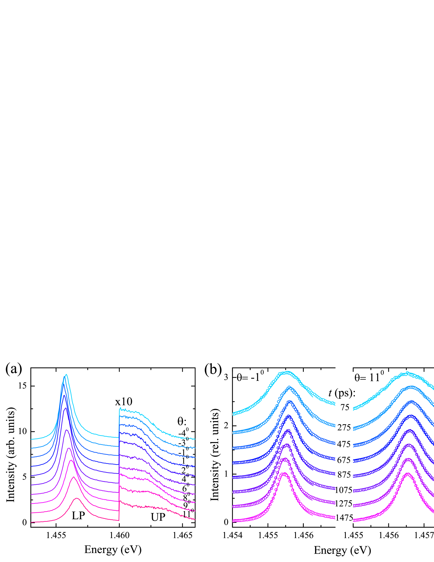
Figure 2: (a) MC emission spectra corresponding to different angles of observation $\Theta$ for $t=275$ ps. Spectra are vertically shifted and intensity values for $E>1.46$ eV are multiplied by 10 for clarity. (b) LP spectra corresponding to different times after the excitation pulse (circles) for two angles of observation. Spectra are normalized to the maximum value and vertically shifted. Solid lines show Lorentzian fits. In (a) and (b) $\Delta=-0.2$ meV, $T_{\text{latt}}=10$ K, nonresonant excitation with $P=1$ mW.

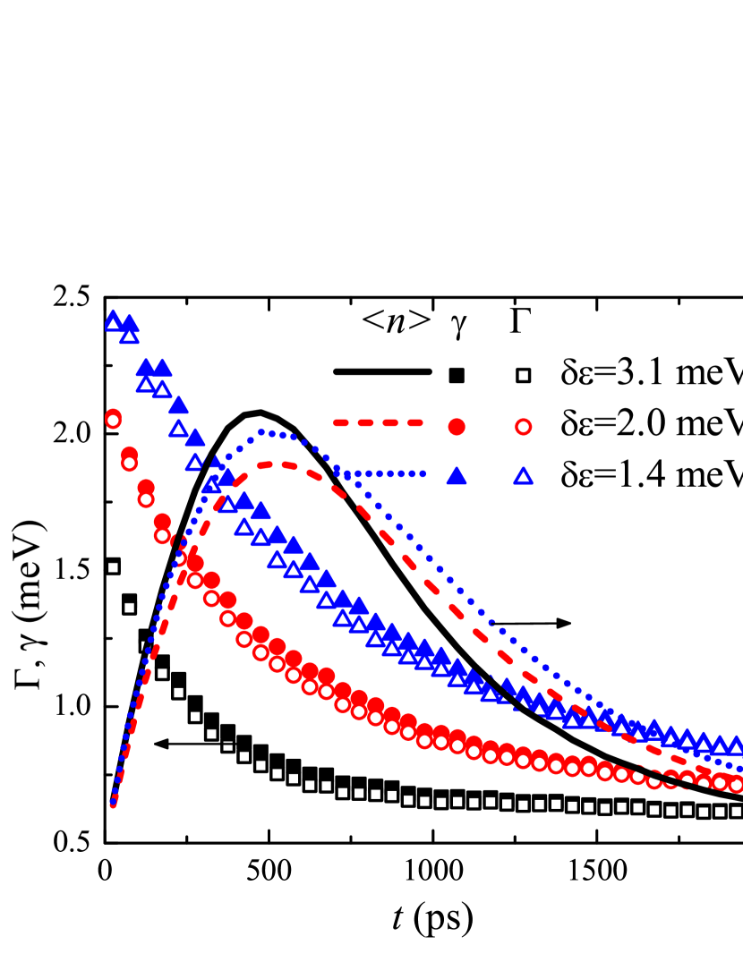
Figure 3: Kinetic dependencies of the LP linewidth $\Gamma$ (open symbols), polariton escape rate $\gamma$ (solid symbols), and population $\langle n\rangle$ (lines, right axis) for different state depths $\delta\varepsilon$. The black squares and solid line correspond to $\Delta=-0.2$ meV, $\Theta=-1^{0}$, the red circles and dashed line correspond to $\Delta=-0.2$ meV, $\Theta=11^{0}$, and the blue triangles and dotted line correspond to $\Delta=2.0$ meV, $\Theta=13^{0}$. Nonresonant excitation with $P=1$ mW, $T_{\text{latt}}=10$ K.

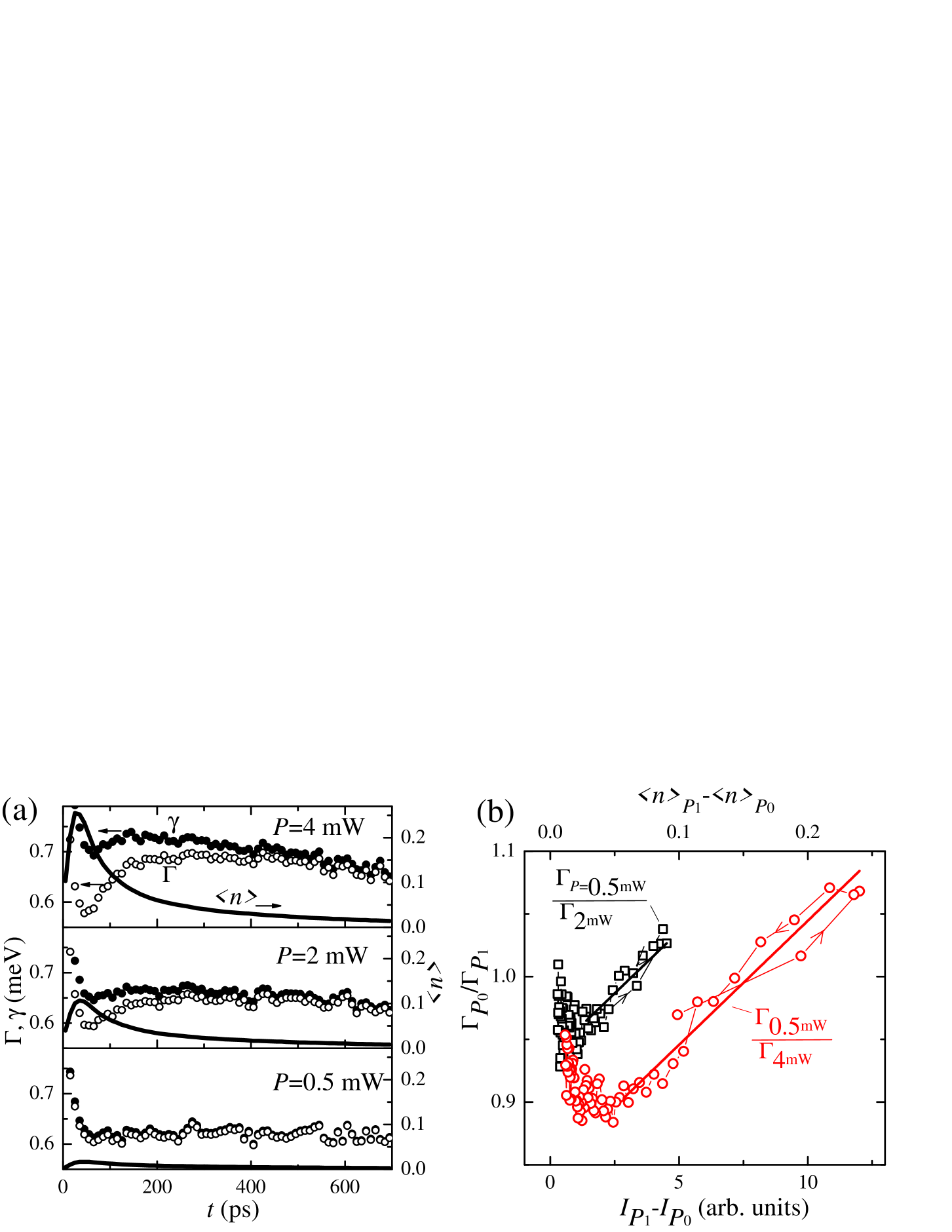
Figure 4: Resonant excitation case. (a) Kinetic dependencies of the LP linewidth $\Gamma$ (open symbols), polariton escape rate $\gamma$ (solid symbols), and population $\langle n\rangle$ (lines, right axis) for different excitation powers $P$. (b) Ratios of the LP linewidths for low, $P_{0}$, and high, $P_{1}$, excitation powers $\Gamma(P_{0})/\Gamma(P_{1})$ as a function of the difference of the intensities $I(P_{1})-I(P_{0})$ (bottom axis) and the difference of the filling factors $\langle n\rangle(P_{1})-\langle n\rangle(P_{0})$ (top axis). Data are presented for $P_{0}=0.5$ mW and two different $P_{1}$, $P_{1}=2$ mW (squares) and $4$ mW (circles). Arrows on the lines connecting data points indicate the direction of increasing time. Thich solid lines show linear fits. In (a) and (b) $\delta\varepsilon=2.1$ meV ($\Delta=2.0$ meV, $\Theta=0^{0}$), $T_{\text{latt}}=10$ K.

The MC emission spectra corresponding to different angles of observation (polariton wave vectors) at time $t=275$ ps after the nonresonant excitation pulse are presented in Fig. 2(a) for the photon-exciton detuning $\Delta=-0.2$ meV. The time-average excitation power $P=1$ mW corresponds to the electron-hole pair density per QW below $5\times 10^{10}$ cm^-2. The spectra show two lines corresponding to the LP and upper polariton (UP) branches, with the characteristic angular dependencies of their energies indicating strong exciton-photon coupling. The measured LP linewidth (FWHM) $\Gamma$ is mainly determined by the rates of polariton scattering and photon escape, the processes giving a Lorentzian intensity distribution, as discussed above. The measurements of the highly photon-like LP linewidth give $\gamma_{\text{c}}\approx 1$ meV. Thus, for $\Delta=-0.2$ meV and $\Theta=-1^{0}$ the contribution of photon escape to the linewidth is $\gamma_{\text{c}}C^{2}\approx 0.5$ meV. Inhomogeneous broadening, mainly related to the QW width fluctuations, and the instrumental response also give some contribution to $\Gamma$ in the form of a Gaussian component. The best fit to the LP line for $\Delta=-0.2$ meV and $\Theta=-1^{0}$ at long $t$ with the Voigt function gives a Lorentzian component width of $\approx 0.5$ meV and a Gaussian component width of $\approx 0.3$ meV, close to $\gamma_{\text{c}}C^{2}$ and the instrumental response function width, respectively. On the other hand, the best fit to the same spectrum with the Lorentzian distribution gives $\Gamma\approx 0.6$ meV. Thus, the relative contribution of the nonhomogeneous sources is small for the considered photon-exciton detunings and observation angles (corresponding to $\delta\varepsilon=1.4-3.1$ meV), especially at shorter times, and further the LP line is fitted by the Lorentzian distribution to determine the FWHM [Fig. 2(b)].

The LP line, broad at short times after the nonresonant excitation pulse, significantly narrows at longer times [Fig. 2(b)]. The narrowing rate varies for different angles of observation, as first pointed out in Ref. Belykh et al. (2012). For the small angle $\Theta=-1^{0}$ ($\delta\varepsilon=3.1$ meV) the linewidth is close to its low-density limit already at $t=475$ ps, while for the larger angle $\Theta=11^{0}$ ($\delta\varepsilon=2.0$ meV) the line continues narrowing for significantly longer times. The LP linewidth $\Gamma$ dynamics for these angles is presented in Fig. 3 by open squares and circles. However, as follows from the theory [Eq. (13)], not $\Theta$ but the state depth $\delta\varepsilon$ is the proper parameter that determines the linewidth dynamics. Indeed, a decrease in $\delta\varepsilon$ achieved by increasing the photon-exciton detuning $\Delta$ leads to the further slowdown of the linewidth kinetics, as shown by open triangles for $\Delta=2.0$ meV and $\Theta=13^{0}$ ($\delta\varepsilon=1.4$ meV). Such behavior of the linewidth kinetics with $\delta\varepsilon$ can be understood from Eq. (13). With increasing $\delta\varepsilon$ the linewidth becomes more sensitive to the reservoir temperature dynamics and decreases much faster with decreasing $T$.

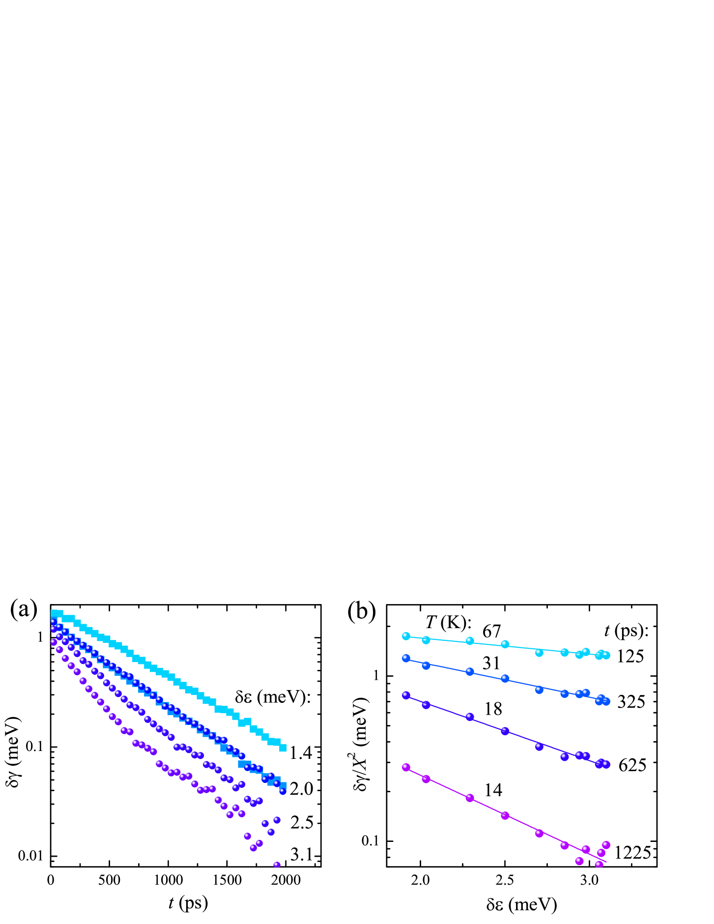
Figure 5: (a) Kinetic dependencies of the time-dependent part $\delta\gamma$ of the polariton escape rate for different state depths $\delta\varepsilon$ corresponding to $\Delta=-0.2$ meV, $\Theta=-1^{0},8^{0},11^{0}$ (circles) and $\Delta=2.0$ meV, $\Theta=5^{0},13^{0}$ (squares). (b) Energy distributions of $\delta\gamma$ normalized to the exciton fraction for different times after the excitation pulse. Solid lines are exponential fits. $\Delta=-0.2$ meV. In (a) and (b) $T_{\text{latt}}=10$ K, nonresonant excitation with $P=1$ mW.

Now we aim to determine the polariton escape rate $\gamma$ from the measured linewidth $\Gamma$. According to Eq. (9), $\gamma=\Gamma(\langle n\rangle+1)$. The mean number $\langle n\rangle$ of polaritons in a single quantum state is proportional to the emission intensity $I$:

$$I=\kappa C^{2}\langle n\rangle,$$ (14)

where $\kappa=\gamma_{\text{c}}\times 2\Delta k_{\text{x}}\Delta k_{\text{y}}A/(2\pi)^{2}\times\omega\times\tilde{\kappa}$ is the photon escape rate times the number of the states from which the intensity is registered times the energy of emitted photons $\omega$, and times a constant $\tilde{\kappa}$ that transforms the real intensity in watts to the intensity measured by the streak camera in arbitrary units; $\Delta k_{\text{x}}$ and $\Delta k_{\text{y}}$ are the wave-vector intervals determined by the angular aperture in which the emission is registered. The coefficient $\kappa$ is independent of $\delta\varepsilon$ and constant in all the considered experiments (we neglect the small variation of $\omega$). To determine $\kappa$, we implement the conditions under which the reduction of $\Gamma$ due to a finite $\langle n\rangle$ is detected directly. For resonant excitation of the LP branch the reservoir is not overheated, in contrast to the nonresonant excitation case, and its temperature is close to the lattice temperature already at short $t$. Thus, the time-dependent contribution to the escape rate $\gamma$ [Eq. (13)] is minimum, and the kinetics of the linewidth $\Gamma$ is dominated by the kinetics of the polariton number $\langle n\rangle$ [denominator in Eq. (13)].

The measured kinetic dependencies of the linewidth for resonant excitation of the PL branch at $\Theta\approx 60^{0}$ with different powers $P$ are presented in Fig. 4 by open symbols. At short times, $\Gamma$ experiences a pronounced drop down proportional to the measured intensity (shown by solid lines, right axis). The intensity has already been transformed to $\langle n\rangle$ by dividing by a constant $\kappa C^{2}$ that will be determined further. An increase in $P$ leads to an enhancement of the intensity and the corresponding increase in the $\Gamma$ drop down. According to Eqs. (13) and (14), $\Gamma(t)^{-1}\approx\gamma_{0}^{-1}[1-\delta\gamma(t)/\gamma_{0}+\langle n\rangle(t)]=\gamma_{0}^{-1}[1-\delta\gamma(t)/\gamma_{0}+I(t)/\kappa C^{2}]$ for $\delta\gamma(t)/\gamma_{0}\ll 1$ and $\langle n\rangle(t)\ll 1$. The linewidth ratio for two excitation powers $P_{0}$ (small) and $P_{1}$ (high),

$$\frac{\Gamma_{P_{0}}(t)}{\Gamma_{P_{1}}(t)}\approx 1-\frac{\delta\gamma_{P_{1}}(t)-\delta\gamma_{P_{0}}(t)}{\gamma_{0}}+\frac{I_{P_{1}}(t)-I_{P_{0}}(t)}{\kappa C^{2}}$$ (15)

allows us to eliminate the systematic error, the line broadening at $t<40$ ps due to the scattered light from higher states. This ratio is proportional to the intensity difference $I_{P_{1}}(t)-I_{P_{0}}(t)$ with the desired coefficient $1/\kappa C^{2}$ in the time range where $I(t)$ varies with $t$ much faster than $\delta\gamma(t)$ ($t\lesssim 200$ ps). Figure 4(b) shows the dependencies of $\Gamma_{P_{0}}/\Gamma_{\text{P}_{1}}$ on $I_{P_{1}}-I_{P_{0}}$ for two different values of $P_{1}$, and the direction of increasing time is indicated by arrows. The dependencies are close to linear for high intensities (at $t\lesssim 200$ ps), as expected from Eq. (15). As the intensity first increases and then decreases with time, the hysteresis in $\Gamma_{P_{0}}/\Gamma_{P_{1}}$ is small. This validates the fact that, in the considered time range, $\delta\gamma(t)$ varies much slower than $I(t)$, and hence, the slope of the linear dependence of $\Gamma_{P_{0}}/\Gamma_{P_{1}}$ on $I_{P_{1}}-I_{P_{0}}$ gives the sought-for coefficient $\kappa C^{2}$. From the linear fits to both the dependencies (thick solid lines) we find $\kappa C^{2}=50\pm 2$. From the measured intensities we calculate with Eq. (14) and the known $C(\varepsilon)^{2}$ the polariton population for all considered states [Figs. 3 and 4(b), right axis]. We note that our method to determine $\langle n\rangle$ is more precise than the direct method based on measuring the emitted intensity Renucci et al. (2005) because the latter method requires knowledge of the exact number of the registered states, which is hard to determine.

Once $\Gamma$ and $\langle n\rangle$ are found, we calculate with Eq. (9) the polariton escape rate $\gamma$, which is shown by solid symbols in Fig. 3 for nonresonant excitation and in Fig. 4(a) for resonant excitation. It is interesting that the time-dependent components of both $\Gamma$ and $\gamma$ for nonresonant excitation are much larger than the corresponding components for resonant excitation for comparable polariton populations. This fact is a good illustration of the reservoir overheating induced by nonresonant excitation and causing the LP line broadening.

Figure 5(a) shows the kinetics of the time-dependent component of the polariton escape rate, $\delta\gamma(t)$, which is determined as the difference of $\gamma(t)$ (solid symbols in Fig. 3) and its value at long $t$. The data are shown for different state depths $\delta\varepsilon$, and changing $\delta\varepsilon$ is performed by increasing the observation angle and photon-exciton detuning [squares and circles in Fig. 5(a) correspond to two different detunings]. For $\delta\varepsilon=2.0$ meV the dependencies corresponding to different detunings almost coincide despite different angles, which confirms that $\delta\varepsilon$ is the proper parameter to define the properties of a polariton state. As $\delta\varepsilon$ is increased, the kinetics of $\delta\gamma$ becomes faster at $t\lesssim 1000$ ps. At longer times the decay of $\delta\gamma$ is more $\delta\varepsilon$ independent. According to Eq. (13),

$$\delta\gamma(t,\delta\varepsilon)\propto[X(\delta\varepsilon)]^{2}N(t)\exp\biggl{(}-\frac{\alpha\delta\varepsilon}{T(t)}\biggr{)},$$ (16)

and the observed behavior of $\delta\gamma$ indicates a strong variation of the reservoir temperature $T$ at $t\lesssim 1000$ ps. The variation becomes smaller at longer times as $T$ relaxes to $T_{\text{latt}}$. To make this description more quantitative, we plot in Fig. 5(b) $\delta\gamma/X^{2}$ as a function of $\delta\varepsilon$ for different times and fixed $\Delta=-0.2$ meV. The dependencies are well described by the exponential function, in accordance with Eq. (16). This allows us to determine the reservoir temperatures $T$ [already indicated in Fig. 5(b)] provided the coefficient $\alpha$ is known. We obtain $\alpha=1.3$ from the condition that $T$ approaches $T_{\text{latt}}$ at long times when $T_{\text{latt}}=20$ K (red solid circles in Fig. 6), and the same value $\alpha=1.3$ is fixed for all the considered $T_{\text{latt}}$ and excitation powers.

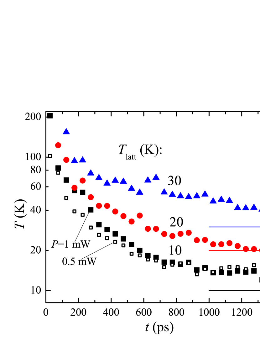
Figure 6: Dynamics of the e-h reservoir temperature for different lattice temperatures $T_{\text{latt}}$ after nonresonant excitation with $P=1$ mW (solid symbols). Open squares show the corresponding dependence for $P=0.5$ mW and $T_{\text{latt}}=10$ K. $\Delta=-0.2$ meV. Horizontal lines indicate the values of $T_{\text{latt}}$.

The time dependencies of the reservoir temperature $T$ for different lattice temperatures $T_{\text{latt}}$ are presented in Fig. 6. At very short times, $T$ is too large to determine; in the time range $t\sim 50-1000$ ps, $T$ changes from about 200 K to the values close to $T_{\text{latt}}$. The fact that at long $t$ the determined reservoir temperature follows $T_{\text{latt}}$ for different values of $T_{\text{latt}}$ is a proof of the validity of our method. Interestingly, for small lattice temperatures, $T$ stays considerably larger than $T_{\text{latt}}$ for several hundreds of picoseconds, in agreement with Refs. Yoon et al. (1996); Leo et al. (1988a, b); Szczytko et al. (2004); Hoyer et al. (2005). For the excitation power $P=0.5$ mW (open squares) the reservoir temperature $T$ at $t\lesssim 1000$ ps is reduced compared with $T$ for $P=1$ mW (solid squares). This observation indicates that the reservoir cooldown is slower for an increased number of particles and can be explained by reabsorption of emitted phonons (hot-phonon bottleneck effect), which is more effective for a denser system Leo et al. (1988a, b); Rosenwaks et al. (1993). Thus, the obtained dynamics of $T$ is very similar to the e-h temperature dynamics reported for bare QW structures Yoon et al. (1996); Leo et al. (1988a, b); Szczytko et al. (2004); Hoyer et al. (2005).

It is instructive to discuss the reservoir temperature dynamics (Fig. 6) in relation to the MC polariton Bose-Einstein condensation. In experiments with GaAs MCs under nonresonant pulsed excitation, BEC is usually observed in the time range $t\lesssim 200$ ps Tempel et al. (2012); Belykh et al. (2013). Our results indicate that in this time range the reservoir is strongly overheated, calling into question the existence of excitons in the BEC regime (however, not canceling the polariton picture Houdré et al. (1994); Tsintzos et al. (2008)) and resulting in the significantly increased BEC threshold and degraded BEC coherence properties in comparison with what one would expect for the reservoir in equilibrium with the lattice. Furthermore, increasing the excitation density well above the threshold leads, on the one hand, to shortening the BEC onset time Belykh et al. (2013) and, on the other hand, to increasing the reservoir temperature for any given time (open and solid squares in Fig. 6). These effects can be one of the reasons leading to the suppression of the condensate spatial coherence for the excitation densities well above the threshold Belykh et al. (2013). It is illustrative that, for the MC structure considered here, further increasing the nonresonant excitation power leads to lasing on the energy of a photon mode Belykh et al. (2012). By contrast, in a similar structure under resonant excitation, and hence with a cold reservoir, the polariton BEC was reported Krizhanovskii et al. (2007).

An interesting conclusion can immediately be drawn from $T\gg T_{\text{latt}}$ at BEC. According to Eq. (2), above the BEC threshold $\gamma\approx w$, which can be rewritten as

$$(w_{\text{xeh}}-\gamma_{\text{xeh}})+(w_{\text{phon}}-\gamma_{\text{phon}})-\gamma_{\text{c}}C^{2}\approx 0,$$ (17)

where $\gamma_{\text{xeh}}=\gamma_{\text{x}}+\gamma_{\text{e}}+\gamma_{\text{h}}$ is the rate of the polariton escape assisted by interparticle interaction ($\gamma_{\text{xeh}}$ coincides with the time-dependent escape rate $\delta\gamma$) and $w_{\text{phon}}$ and $w_{\text{xeh}}$ are the rates of the polariton scattering assisted by phonons and interparticle interaction to the given state. Since the general expression (2) for the mean polariton number reduces to the Bose-Einstein distribution $\{\exp[(E-\mu)/T]-1\}^{-1}$ when the state interacts solely with the equilibrium reservoir (which formally corresponds to $\gamma_{\text{c}}C^{2}=\gamma_{\text{phon}}=w_{\text{phon}}=0$), we have

$$w_{\text{xeh}} = \gamma_{\text{xeh}}\exp\biggl{(}-\frac{E-\mu}{T}\biggr{)},$$ (18)

where $\mu$ is the chemical potential for the exciton part of the reservoir. Alternatively, this equation can be derived by calculating $\gamma_{\text{xeh}}$ and $w_{\text{xeh}}$ in the Born approximation. It is easy to show that for a nondegenerate reservoir

$$\exp\biggl{(}-\frac{E-\mu}{T}\biggr{)}\approx\frac{2\pi N_{\text{x}}}{g_{\text{x}}m_{\text{x}}T}\exp\biggl{(}\frac{\delta\varepsilon}{T}\biggr{)}.$$

Taking the realistic parameters for a GaAs structure $\delta\varepsilon=5$ meV, $m_{\text{x}}=0.3m_{0}$ (two-dimensional exciton effective mass Hillmer et al. (1989)), where $m_{0}$ is the free electron mass, $g_{\text{x}}=4$, and taking the reservoir temperature $T=60$ K at $t\sim 100$ ps (Fig. 6), we obtain $\exp[-(E-\mu)/T]\approx N_{\text{x}}\times(2\times 10^{-12}$ cm${}^{2})<1$ because the polariton BEC implies the strong coupling regime and, thus, the unsaturated reservoir, $a_{\text{B}}^{2}N_{\text{x}}\ll 1$, where the exciton Bohr radius is $a_{\text{B}}\sim 10^{-6}$ cm. With Eq. (18), we conclude that the rate of polariton scattering to the given state due to interparticle interaction is smaller than the corresponding polariton escape rate:

$$w_{\text{xeh}}<\gamma_{\text{xeh}}.$$ (19)

As a result, the first term in Eq. (17) is negative; therefore, polariton escape in the regime of BEC is compensated only by the phonon-assisted polariton relaxation. Thus, contrary to the common belief, for nonresonant excitation, interparticle interaction drives polaritons away from the condensate rather than promoting their condensation.

Condition (19) might be violated for too deep states [note $\exp[-(E-\mu)/T]\propto\exp(\delta\varepsilon/T)$], e.g., for $\delta\varepsilon>13$ meV at $N_{\text{x}}=10^{11}$ cm^-2 or $\delta\varepsilon>25$ meV at $N_{\text{x}}=10^{10}$ cm^-2. These values of $\delta\varepsilon$ are relatively large for BEC in GaAs MCs Belykh et al. (2013); Tempel et al. (2012); Balili et al. (2007); Krizhanovskii et al. (2007); Wertz et al. (2009); Kammann et al. (2012) but are easily achievable for the MCs based on materials with larger exciton binding energy and Rabi splitting, such as CdTe Kasprzak et al. (2006, 2008); del Valle et al. (2009), GaN Christopoulos et al. (2007); Levrat et al. (2010), and ZnO Li et al. (2013). In this case condition (19) can be satisfied at positive photon-exciton detunings in the so-called thermodynamic condensation regime Kasprzak et al. (2008); Levrat et al. (2010).

Condition (19) does not contradict the well-established importance of interparticle interaction in polariton relaxation for relatively high excitation densities for the noncondensed regime Tartakovskii et al. (2000); Belykh et al. (2011); Bajoni et al. (2006); Qarry et al. (2003). Indeed, in the rate equation the income term describing polariton scattering assisted by interparticle interaction is $w_{\text{xeh}}(1+\langle n\rangle)$ whereas the corresponding term describing polariton escape is $\gamma_{\text{xeh}}\langle n\rangle$. For $\langle n\rangle\ll 1$, the income term can dominate despite the condition (19). The situation is reversed for the regime of condensation, when $\langle n\rangle\gg 1$. Furthermore, our conclusion does not contradict the reported enhancement of polariton relaxation due to reservoir heating Tartakovskii et al. (2003) because the value of $w_{\text{xeh}}$ grows with the reservoir temperature [Eqs. (11), (12), and (18)].

V Conclusion

We have studied theoretically and experimentally the polariton linewidth and have shown that it is determined by the polariton escape rate and polariton population. In experiments with resonant excitation, the dynamics of the polariton linewidth is mainly governed by the dynamics of the occupation number. By contrast, in experiments with nonresonant excitation, this dynamics is mainly governed by the dynamics of the polariton escape rate, which in turn is governed by the dynamics of the reservoir temperature. On this basis, we have developed a method of determining the reservoir temperature by tracing the dependence of the polariton escape rate on the polariton energy. The extracted reservoir temperature for nonresonant pulsed excitation of a GaAs microcavity decays from $\sim 100$ K at $50-100$ ps to the lattice temperature in a time of $\sim 1$ ns. Increasing the excitation power leads to a slowdown of the reservoir temperature relaxation. We have concluded that, in experiments with nonresonant pulsed excitation of GaAs microcavities, the reservoir temperature greatly exceeds the lattice temperature in the regime of the polariton Bose-Einstein condensation. As a result, the condensation is governed by the phonon-assisted polariton relaxation, while the overall effect of interparticle scattering is depopulation of the condensate.