When will the crossing number of an alternating link decrease by two via a crossing change?

Abstract

Let $D$ be a reduced alternating diagram of a non-split link $L$ and $\tilde{L}$ be the link whose diagram is obtained from $D$ by a crossing change. If $\tilde{L}$ is alternating, then $c(\tilde{L})\leq c(L)-2$. In this paper we explore when $c(\tilde{L})=c(L)-2$ holds and obtain a simple sufficient and necessary condition in terms of plane graphs corresponding to $L$. This result is obtained via analyzing the behavior of the Tutte polynomial of the signed plane graph corresponding to $\tilde{L}$.

1 Introduction

Let $L$ be a link. We denote by $c(L)$ the crossing number of the link $L$, that is, the smallest number of crossings, the minimum being taken over all diagrams of $L$. Let $D$ be a diagram, by a crossing change we mean exchanging the over-pass and the under-pass curves at a single crossing of $D$. The crossing number of an alternating link may decrease dramatically via a single crossing change, for example, alternating knots with unknotting number one as shown in Fig. 1. It is natural to ask which conditions should be satisfied by an alternating knot diagram such that its crossing number decreases only a little when one changes any its crossing. It is well known that there is a one-to-one correspondence between link diagrams and signed plane graphs via the medial construction, which provide a method of studying knots using graphs [1]. We shall answer this question in terms of corresponding plane graphs under some moderate conditions.

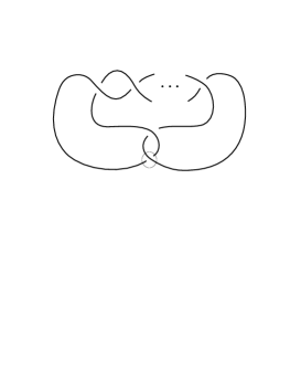
Fig. 1: By changing the crossing circled, the alternating knot is unknotted.

Another inspiration for our study is works of ordering knots via crossing changes. In [6], Diao et al defined a partial ordering of links using a property derived from their minimal diagrams. A link $L^{\prime}$ is called a predecessor of a link $L$ if $c(L^{\prime})<c(L)$ and a diagram of $L^{\prime}$ can be obtained from a minimal diagram $D$ of $L$ by a single crossing change. In addition, in [18], Taniyama defined that $L_{1}$ is a major of $L_{2}$ if every diagram of $L_{1}$ can be transformed into a diagram of $L_{2}$ by applying crossing changes at some crossings of the diagram of $L_{1}$. The notion of major is extended to $s$-major in [7] via adding smoothing operations by Endo et al. Our result may help to their studies.

We noted the following result obtained by L. Wu et al.

Theorem 1.1

[21] Let $L$ be a non-split link which admits a reduced alternating diagram $D$. Let $\tilde{L}$ be the link obtained from $D$ by a crossing change. If $\tilde{L}$ is alternating, then

$$c(\tilde{L})\leq c(L)-2.$$ (1)

Theorem 3.2 in [6] shows that Theorem 1.1 holds for rational links. In this paper we shall explore when the equality in Theorem 1.1 holds, that is, when the crossing number of an alternating link decreases by two via a crossing change?

We attempt to study the effect of crossing number of a link after a single crossing change and find that it is difficult to deal with it by using the diagrammatic approach. However, when we turn to the corresponding plane graphs, the Tutte polynomial of graphs or signed graphs provides a good tool to solve the problem. Let $G$ be a graph. The multiplicity $\mu(e)$ of an edge $e=(u,v)$ of $G$ is the number of all edges with end-vertices $u$ and $v$. We use $N(v)$ to denote the set of all vertices of $G$ that have a common edge with $v$. In this paper we proved

Theorem 1.2

Let $G$ be a connected bridgeless and loopless positive plane graph and $e=(u,v)$ be an edge of $G$. Let $L$ be the alternating link corresponding to $G$ and $\tilde{L}$ be the link corresponding to $\tilde{G}$ obtained from $G$ by changing the sign of $e$ from $+$ to $-$. Suppose that $L$ is non-split and $\tilde{L}$ is alternating, we have

1. if $\tilde{L}$ is split, then $c(\tilde{L})=c(L)-2$ if and only if $\mu(e)=2$ and if we suppose that $f$ is the edge parallel to $e$, then $G-e-f$ is disconnected.

2. if $\tilde{L}$ is non-split, then $c(\tilde{L})=c(L)-2$ if and only if one of the following two conditions holds:

   1. $\mu(e)=1$, $G-e$ has bridges and $N(u)\cap N(v)=\emptyset$.

   2. $\mu(e)>1$ and if we suppose that $f$ is an edge parallel to $e$, then $G-e-f$ is connected and bridgeless.

Note that the characterization of plane graphs corresponding to knots has been given in [17, 8, 9]. In the following of this section, we apply Theorem 1.2 to the case of knots. A graph is said to be 2-edge connected if it is connected and bridgeless. An edge with multiplicity 1 or a (not necessarily maximal) multiple edge, which is formally defined in Section 4, of a 2-edge connected graph $G$ is said to be reducible if $G$ is still 2-edge connected after deleting the edge or the multiple edge, otherwise it is said to be irreducible. A triangle in a graph $G$ is called to be quasi-simple if it has at least one edge with multiplicity 1.

Corollary 1.3

Let $G$ be a connected bridgeless and loopless positive plane graph. Let $L$ be the alternating link corresponding to $G$ and $\tilde{L}$ be any link corresponding to $\tilde{G}$ obtained from $G$ by changing the sign of an edge of $G$ from $+$ to $-$. Suppose that $L$ is a knot and $\tilde{L}$ is always alternating. Then $c(\tilde{L})=c(L)-2$ for any $\tilde{L}$ if and only if

1. $G$ is quasi-simple triangle free,

2. each edge with multiplicity 1 is irreducible,

3. A pair of edges in any maximal multiple edge is reducible.

Proof. Since $L$ is a knot, $\tilde{L}$ is also a knot. Hence both $L$ and $\tilde{L}$ are non-split. Let $e$ be an edge of $G$. If $\mu(e)=1$, Conditions 1 and 2 are equivalent to Theorem 1.2 2(1). If $\mu(e)>1$, Condition 3 is equivalent to Theorem 1.2 2(2). $\Box$

A 2-edge connected graph $G$ is said to be minimal if, for each edge $e$ of $G$, $G-e$ has bridges. We further restrict ourselves to simple graphs, that is, graphs having no loops or multiple edges, and, as a direct consequence of Corollary 1.3, we obtain

Corollary 1.4

Let $G$ be a connected bridgeless and loopless positive simple plane graph. Let $L$ be the alternating link corresponding to $G$ and $\tilde{L}$ be any link corresponding to $\tilde{G}$ obtained from $G$ by changing the sign of an edge of $G$ from $+$ to $-$. Suppose that $L$ is a knot and $\tilde{L}$ is always alternating. Then $c(\tilde{L})=c(L)-2$ for any $\tilde{L}$ if and only if $G$ is a triangle-free and minimal 2-edge connected graph.

Compared with Theorem 1.2, Corollaries 1.3 and 1.4 can both be viewed as results on the ’whole’ alternating link diagram. For the construction and properties of minimal 2-edge connected graph, see [22, 5].

The paper is organized as follows. In Section 2, we provide some preliminary knowledge, including the relation between the crossing number of an alternating link and the span of its Jones polynomial, and the relation between the Jones polynomial and the Tutte polynomial. We then give a graph-theoretic proof of Theorem 1.1 in Section 3. In Section 4, we obtain a ’dual’ result of Dasbach and Lin [14] on the coefficients of $T_{G}(-t,-t^{-1})$. Theorem 1.2 is thus obtained by studying the proof in Section 3 and using the ’dual’ result and its proof is given in Section 5. In the final Section 6, we give an example illustrating Theorem 1.2 and pose two problems for further study.

2 Preliminaries

The readers who are familiar with the knowledge on the correspondence between graphs and links, Jones polynomial and Tutte polynomial can skip this section.

2.1 Some terminologies and notations

A graph $G$ is a pair of sets $V(G)$ and $E(G)$, where $V(G)$ is a non-empty finite set (of vertices) and $E(G)$ is a multi-set of unordered pairs $(x,y)$ (not necessarily distinct) of vertices called edges. An edge with unordered pair $(x,x)$ is called a loop. For $v\in V(G)$, let $N(v)=\{u\in V(G)|(u,v)\in E(G)\}-\{v\}$. Graphs can be represented graphically, that is, we can draw it as follows: each vertex is indicated by a point, and each edge $(x,y)$ by a line joining the points $x$ and $y$. A graph is planar if it can be embedded in the plane, that is, it can be drawn on the plane so that no two edges intersect. A plane graph is a particular plane embedding of a planar graph. A graph is said to be trivial if it consists of only an isolated vertex without loops. A signed graph is a graph each of whose edges is labeled with a sign ($+$ or $-$).

A graph is said to be connected if, for any its two distinct vertices $u,v$, there is a path $u=u_{0}u_{1}u_{2}\cdots u_{l}=v$, where $u_{i}$ ($i=0,1,\cdots,l$) are all distinct and $(u_{i-1},u_{i})$ is an edge for $i=1,2,\cdots,l$. A connected component of a graph is a maximal connected subgraph of the graph. A bridge of a graph $G$ is an edge whose removal would increase the number of connected components of $G$. By contracting an edge we mean deleting the edge firstly and then identifying its end-vertices. Let $e$ be an edge of $G$. We shall denote by $G-e$ and $G/e$ the graph obtained from $G$ by deleting and contracting the edge $e$, respectively. When $G$ is a plane graph, $G-e$ and $G/e$ are also plane graphs obtained in a natural way.

A knot is a simple closed piecewise linear curve in Euclidean 3-space $\mathbb{R}^{3}$. A link is the disjoint union of finite number of knots, each knot is called a component of the link. We take the convention that a knot is a one-component link. We can always represent links in $R^{3}$ by link diagrams in a plane, that is, regular projections with a short segment of the underpass curve cut at each double point of the projection.

A link diagram is said to be split if it is a composition of the diagrams of two links with no points in common [15], and otherwise non-split or connected. A link that has a split diagram is said to be a split link, and otherwise non-split or connected. A link diagram is said to be alternating if over- and under-crossings alternate as one travels the link (crossing at the crossings), and otherwise non-alternating. A link is said to be alternating if it has an alternating link diagram, and otherwise non-alternating. A nugatory crossing of a link diagram is a crossing in the diagram so that two of the four local regions at the crossing are part of the same region in the larger diagram. A reduced diagram is one that does not contain nugatory crossings.

2.2 Links and graphs

The 1-1 correspondence between link diagrams and signed plane graphs has been known for about one hundred years. It was once one of the methods used by Tait and Little in the late 19th century to construct a table of knot diagrams of all knots starting with graphs with a relatively small number of edges and then increasing the number of edges [15]. To describe this correspondence, we first recall the medial graph of a plane graph.

Definition 2.1

The medial graph $M(G)$ of a non-trivial connected plane graph $G$ is a 4-regular plane graph obtained by inserting a vertex on every edge of $G$, and joining two new vertices by an edge lying in a face of $G$ if the vertices are on adjacent edges of the face; if $G$ is trivial, its medial graph is defined to be a simple closed curve surrounding the vertex (strictly, it is not a graph); if a plane graph $G$ is not connected, its medial graph $M(G)$ is defined to be the disjoint union of the medial graphs of all its connected components.

Given a signed plane graph $G$, we first draw its medial graph $M(G)$. To turn $M(G)$ into a link diagram $D(G)$, we turn the vertices of $M(G)$ into crossings by defining a crossing to be over or under according to the sign of the edge as shown in Fig. 2. Conversely, given a connected link diagram $D$, shade it as in a checkerboard so that the unbounded face is unshaded. Note that such a shading is always possible, since link diagrams can be viewed as 4-regular plane graphs, see Exercise 9.6.1 of [4]. We then associate $D$ with a signed plane graph $G(D)$ as follows: For each shaded face $F$, take a vertex $v_{F}$, and for each crossing at which $F_{1}$ and $F_{2}$ meet, take an edge $(v_{F_{1}},v_{F_{2}})$ and give the edge a sign also as shown in Fig. 2. if a link diagram $D$ is not connected, its corresponding signed plane graph $G(D)$ is defined to be the disjoint union of the signed plane graphs of all its connected components.

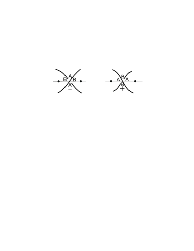
Fig. 2: The correspondence between a crossing and a signed edge [13].

Under the 1-1 correspondence described above, there is also an 1-1 correspondence between crossings of $D$ and edges of $G(D)$. The following three properties on the correspondence are all obvious.

P1: $D$ is a connected link diagram if and only if its corresponding signed plane graph $G(D)$ is connected.

P2: A crossing of $D$ is nugatory if and only if its corresponding edge in $G(D)$ is a loop or a bridge. Furthermore, $D$ is reduced if and only if $G(D)$ is loopless and bridgeless.

P3: $D$ is alternating if and only if all edges of $G(D)$ have the same signs.

2.3 Jones and Tutte polynomials

Let $L$ be an oriented link, $V_{L}(t)$ be the Jones polynomial [10] of $L$. We denote by $span_{v}(L)$ the difference between the maximal and minimal degrees of $V_{L}(t)$, i.e.

$$span_{v}(L)=\max\deg V_{L}(t)-\min\deg V_{L}(t).$$

In [11], Kauffman introduced the Kauffman bracket polynomial of unoriented link diagrams. Let $D$ be an unoriented link diagram. Let $[D]=[D](A,B,d)$ be the Kauffman square bracket polynomial of $D$, $<D>\ =[D](A,A^{-1},-A^{2}-A^{-2})$ be the Kauffman bracket polynomial of $D$. We denote by $span_{k}(D)$ the difference between the maximal and minimal degrees of $<D>$, i.e.

$$span_{k}(D)=\max\deg<D>-\min\deg<D>.$$

Let $L$ be an oriented link, $D$ be an oriented diagram of $L$. The writhe $w(D)$ of $D$ is defined to be the sum of signs of the crossings of $D$. Kauffman proved [11, 12]

$$V_{L}(t)=(-A^{3})^{-w(D)}<D>|_{A=t^{-1/4}}.$$

Hence we have

$$span_{v}(L)={1\over 4}span_{k}(D).$$ (2)

Lemma 2.2

[11, 16, 19] Let $D$ be a unoriented diagram of an oriented link $L$.

1. If $L$ is a non-split alternating link, then $c(L)=span_{v}(L)={1\over 4}span_{k}(D)$.

2. If $L$ is a split alternating link with $n(L)$ non-split components, then $c(L)=span_{v}(L)-n(L)+1={1\over 4}span_{k}(D)-n(L)+1$.

Given a crossing of a link diagram, we can distinguish two out of the four small regions incident at the crossing. Rotate the over-crossing arc counterclockwise until the under-crossing arc is reached, and call the small two regions swept out the $A$-channels and other two the $B$-channels. For example, in Fig. 2, the edge with sign $+$(resp. $-$) edge crosses $A$-channels (resp. $B$-channels). In the case of an alternating link diagram, each of its regions has only $A$-channels or only $B$-channels. Calling a region an $A$-region if all its channels are $A$ channels, and a $B$-region if all its channels are $B$ channels.

Lemma 2.3

[11, 12] Let $D$ be a connected reduced alternating link diagram. Then

1. $\max\deg<D>\ =V+2W-2$, where $V$ is the number of crossings of $D$ and $W$ is the number of $B$-regions. The coefficient of this power of $A$ in $<D>$ is $(-1)^{W-1}$.

2. $\min\deg<D>\ =-V-2B+2$, where $V$ is the number of crossings of $D$ and $B$ is the number of $A$-regions. The coefficient of this power of $A$ in $<D>$ is $(-1)^{B-1}$.

Motivated by the 1-1 correspondence between link diagrams and signed plane graphs, in [13] Kauffman constructed a Tutte polynomial for signed graphs, which is generalizations of both the Tutte polynomial [20] for ordinary graphs and the Kauffman square bracket polynomial. Let $G$ be a signed graph and $Q[G]=Q[G](A,B,d)$ be the Tutte polynomial of $G$, which we shall call the $Q$-polynomial for clarity.

Definition 2.4

The $Q$-polynomial can be defined by the following recursive rules:

1. Let $E_{n}$ be the edgeless graph with $n$ vertices. Then

   $$Q[E_{n}]=d^{n-1}.$$

2. 1. If $e$ is a bridge, then

      $$Q[G]=(A+Bd)Q[G/e]\ {when}\ s(e)=+\ and$$

      $$Q[G]=(B+Ad)Q[G/e]\ {when}\ s(e)=-.$$

   2. If $e$ is a loop, then

      $$Q[G]=(B+Ad)Q[G-e]\ {when}\ s(e)=+\ and$$

      $$Q[G]=(A+Bd)Q[G-e]\ {when}\ s(e)=-.$$

   3. If $e$ is neither a bridge nor a loop, then

      $$Q[G]=BQ[G-e]+AQ[G/e]\ {when}\ s(e)=+\ and$$

      $$Q[G]=AQ[G-e]+BQ[G/e]\ {when}\ s(e)=-.$$

Lemma 2.5

[13] Let $G$ be a signed plane graph, $D(G)$ be the link diagram corresponding to $G$. Then $Q[G]=[D(G)]$.

Let $G$ be a signed plane graph. The componentwise dual $G^{*}$ of $G$ is defined to be the disjoint union of the dual graphs of all connected components of $G$. Note that there is a bijection between edges of $G$ and edges of $G^{*}$, and the edge $e\in E(G)$ and the corresponding edge $e^{*}\in E(G^{*})$ receive opposite signs.

Lemma 2.6

Let $G$ be a signed plane graph, $G^{*}$ be the componentwise dual of $G$. Then $Q[G]=Q[G^{*}]$.

From now on we always suppose that $Q[G]=Q[G](A,A^{-1},-A^{2}-A^{-2})$. Recall that the Tutte polynomial $T_{G}(x,y)$ of a graph $G=(V,E)$ can be defined by the following summation:

$$\sum_{F\subseteq E}(x-1)^{k(F)-1}(y-1)^{|F|-|V|+k(F)},$$ (3)

where $k(F)$ is the number of connected components of the spanning subgraph $(V,F)$ of $G$.

A signed graph $G$ is said to be positive (resp. negative) if any of its edges receives a positive (resp. negative) sign. Using the Receipe Theorem of the Tutte polynomial [3] or Thistlethwaite Theorem [19], we can deduce

Lemma 2.7

Let $G=(V,E)$ be a connected graph, $G_{+}$ be the positive graph whose underlying graph is $G$. Then

$$Q[G_{+}]=A^{-|E|+2|V|-2}T_{G}(-A^{-4},-A^{4}).$$

3 The proof of Theorem 1.1

Let $L$ be a non-split link which admits a reduced alternating diagram $D$. Since $L$ is non-split, $D$ must be also connected. Let $G=G(D)$ be the signed plane graph corresponding to $D$. Without loss of generality we assume that $G$ is positive. Otherwise, by Lemma 2.6 we shall work on $G^{*}$. Since $D$ is reduced, $G$ is loopless and bridgeless.

Let $\tilde{L}$ be an alternating link whose diagram $\tilde{D}$ is obtained from $D$ by a crossing $c$ change. Since $D$ is connected, $\tilde{D}$ is also connected. Let $\tilde{G}=G(\tilde{D})$ be the signed plane graph corresponding to $\tilde{D}$. Then $\tilde{G}$ can be obtained from $G$ by changing the sign of an edge $e$ corresponding to $c$ from $+$ to $-$.

Let $span_{q}(\tilde{G})=\max\deg Q[\tilde{G}]-\min\deg Q[\tilde{G}]$. By Lemmas 2.2 and 2.5, we have

$$c(\tilde{L}) \leq span_{v}(\tilde{L})$$ (4)

$$= {1\over 4}span_{q}(\tilde{G}).$$

By Definition 2.4 and note that the sign of the edge $e$ in $G$ (resp. $\tilde{G}$) is positive (resp. negative), we have

$$Q[\tilde{G}]=AQ[G^{\prime}]+A^{-1}Q[G^{\prime\prime}],$$

$$Q[G]=A^{-1}Q[G^{\prime}]+AQ[G^{\prime\prime}],$$

where $G^{\prime}=G-e$ and $G^{\prime\prime}=G/e$. Hence we obtain

$$Q[\tilde{G}]=A^{2}Q[G]+(A^{-1}-A^{3})Q[G^{\prime\prime}]$$ (5)

or

$$Q[\tilde{G}]=A^{-2}Q[G]+(A^{1}-A^{-3})Q[G^{\prime}].$$ (6)

Since $G$ is loopless and bridgeless, it is clear that $G^{\prime}=G-e$ is loopless and $G^{\prime\prime}=G/e$ is bridgeless.

Case 1. $G^{\prime\prime}$ is loopless.

In this case $G^{\prime\prime}$ is connected, loopless, bridgeless and positive, hence the link diagram corresponding to $G^{\prime\prime}$ is connected, reduced and alternating. Let $H$ be a connected plane graph, we shall use $v(H),e(H)$ and $f(H)$ to denote the number of vertices, edges and faces of $H$, respectively. By Lemma 2.3, we have:

1. $\max\deg Q[G]=\max\deg<D>\ =V+2W-2=e(G)+2f(G)-2$ and the corresponding coefficient of this power is $(-1)^{f(G)-1}$.

2. $\min\deg Q[G]=\min\deg<D>\ =-V-2B+2=-e(G)-2v(G)+2$ and the corresponding coefficient of this power is $(-1)^{v(G)-1}$.

3. $\max\deg Q[G^{\prime\prime}]=e(G^{\prime\prime})+2f(G^{\prime\prime})-2=e(G)+2f(G)-3$ and the corresponding coefficient of this power is $(-1)^{f(G^{\prime\prime})-1}=(-1)^{f(G)-1}$.

4. $\min\deg Q[G^{\prime\prime}]=-e(G^{\prime\prime})-2v(G^{\prime\prime})+2=-e(G)-2v(G)+5$ and the corresponding coefficient of this power is $(-1)^{v(G^{\prime\prime})-1}=(-1)^{v(G)}$.

Hence,

1. $\max\deg A^{2}Q[G]=e(G)+2f(G)$ and the corresponding coefficient of this power is $(-1)^{f(G)-1}$.

2. $\min\deg A^{2}Q[G]=-e(G)-2v(G)+4$ and the corresponding coefficient of this power is $(-1)^{v(G)-1}$.

3. $\max\deg(A^{-1}-A^{3})Q[G^{\prime\prime}]=e(G)+2f(G)$ and the corresponding coefficient of this power is $(-1)^{f(G)}$.

4. $\min\deg(A^{-1}-A^{3})Q[G^{\prime\prime}]=-e(G)-2v(G)+4$ and the corresponding coefficient of this power is $(-1)^{v(G)}$.

Note that the maximal (resp. minimal) degree terms of $A^{2}Q[G]$ and $(A^{-1}-A^{3})Q[G^{\prime\prime}]$ cancel each other. Therefore, by Eq. (5), we have

$$\max\deg Q[\tilde{G}] \leq e(G)+2f(G)-4,$$

$$\min\deg Q[\tilde{G}] \geq -e(G)-2v(G)+8.$$

So,

$$span_{q}(G)=\max\deg Q[G]-\min\deg Q[G]=2e(G)+2f(G)+2v(G)-4,$$

and

$$span_{q}(\tilde{G}) = \max\deg Q[\tilde{G}]-\min\deg Q<\tilde{G}>$$

$$\leq 2e(G)+2f(G)+2v(G)-12$$

$$= span_{q}(G)-8.$$

Hence,

$$c(\tilde{L}) \leq {1\over 4}span_{q}(\tilde{G})$$

$$\leq {1\over 4}span_{q}(G)-2$$

$$= c(L)-2.$$

Case 2. $G^{\prime\prime}$ has loops.

Let $f$ be any loop of $G^{\prime\prime}$. Since $G$ is loopless, $f$ must be an edge of $G$ parallel to $e$. There are two subcases:

Case 2a. If $G-e-f=G^{\prime}-f$ is disconnected, then $\tilde{G}-e-f$ is disconnected. So $\tilde{D}$ can be split as shown in Fig. 3, which reduces the crossing number by two. Hence, Theorem 1.1 holds.

Case 2b. If $G-e-f=G^{\prime}-f$ is connected.

Now we prove $G^{\prime}$ is bridgeless. Firstly $f$ is not a bridge of $G^{\prime}$ and let $g\neq f$ be an edge of $G^{\prime}=G-e$. Since $G$ is bridgeless, $g$ belongs to a cycle $C$ of $G$. If $e\notin E(C)$, $g$ belongs to a cycle $C$ of $G^{\prime}$; If $e\in E(C)$, $g$ belongs to a cycle $C^{\prime}=C-e+f$ of $G^{\prime}$. Thus $g$ is not a bridge. Hence $G^{\prime}$ is connected, loopless, bridgeless and positive.

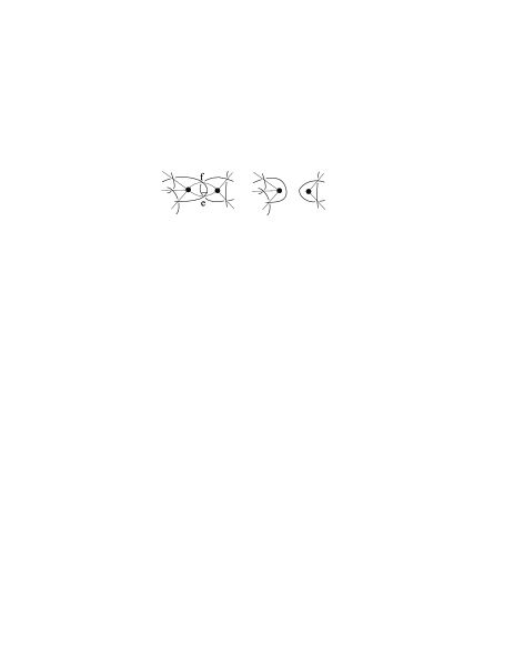
Fig. 3: The case $G-e-f$ is disconnected.

Similarly, by Lemma 2.3, we have:

1. $\max\deg Q[G]=\max\deg<D>\ =V+2W-2=e(G)+2f(G)-2$ and the corresponding coefficient of this power is $(-1)^{f(G)-1}$.

2. $\min\deg Q[G]=\min\deg<D>\ =-V-2B+2=-e(G)-2v(G)+2$ and the corresponding coefficient of this power is $(-1)^{v(G)-1}$.

3. $\max\deg Q[G^{\prime}]=e(G^{\prime})+2f(G^{\prime})-2=e(G)+2f(G)-5$ and the corresponding coefficient of this power is $(-1)^{f(G^{\prime})-1}=(-1)^{f(G)}$.

4. $\min\deg Q[G^{\prime}]=-e(G^{\prime})-2v(G^{\prime})+2=-e(G)-2v(G)+3$ and the corresponding coefficient of this power is $(-1)^{v(G^{\prime})-1}=(-1)^{v(G)-1}$.

Hence,

1. $\max\deg A^{-2}Q[G]=e(G)+2f(G)-4$ and the corresponding coefficient of this power is $(-1)^{f(G)-1}$.

2. $\min\deg A^{-2}Q[G]=-e(G)-2v(G)$ and the corresponding coefficient of this power is $(-1)^{v(G)-1}$.

3. $\max\deg(A^{1}-A^{-3})Q[G^{\prime}]=e(G)+2f(G)-4$ and the corresponding coefficient of this power is $(-1)^{f(G)}$.

4. $\min\deg(A^{1}-A^{-3})Q[G^{\prime}]=-e(G)-2v(G)$ and the corresponding coefficient of this power is $(-1)^{v(G)}$.

Note that the maximal (resp. minimal) degree terms of $A^{-2}Q[G]$ and $(A^{1}-A^{-3})Q[G^{\prime}]$ cancel each other. Therefore, by Eq. (6), we have

$$\max\deg Q[\tilde{G}] \leq e(G)+2f(G)-8,$$

$$\min\deg Q[\tilde{G}] \geq -e(G)-2v(G)+4.$$

Thus,

$$span_{q}(\tilde{G}) = \max\deg Q[\tilde{G}]-\min\deg Q[\tilde{G}]$$

$$\leq 2e(G)+2f(G)+2v(G)-12$$

$$= span_{q}(G)-8.$$

Hence,

$$c(\tilde{L}) \leq {1\over 4}span_{q}(\tilde{G})$$

$$\leq {1\over 4}span_{q}(G)-2$$

$$= c(L)-2.$$

This completes the proof of Theorem 1.1. $\Box$

4 A ’dual’ result

Let $G=(V,E)$ be a connected loopless graph. $I\subset E$ is said to be a multiple edge if $|I|\geq 2$ and any two of $I$ have the same end-vertices. A multiple edge $I_{M}$ is said to be maximal if no multiple edge contains it as a proper subset. In [14], Dasbach abd Lin proved the following lemma.

Lemma 4.1

Let $G=(V,E)$ be a connected loopless graph. Let the Tutte polynomial evaluation

$$T_{G}(-t,-t^{-1})=a_{n}t^{n}+a_{n+1}t^{n+1}+\cdots+a_{m-1}t^{m-1}+a_{m}t^{m}$$

with $a_{n}\neq 0,a_{m}\neq 0$ and $n\leq m$. Then $m=|V|-1$ and

1. $a_{m}=(-1)^{|V|-1}$.

2. $a_{m-1}=(-1)^{|V|-1}(|V|-1-|E|+\sum_{I_{M}}(|I_{M}|-1))$, where $I_{M}$ is a maximal multiple edge and the summation is over all maximal multiple edges.

Let $E_{s}$ be the edge set of $G_{s}$, the graph obtained from $G$ by replacing each maximal multiple edge by a single edge. Then $a_{m-1}=(-1)^{|V|-1}(|V|-1-|E_{s}|)$. In the following of this section, we investigate the value of $n$ and the two coefficients $a_{n}$ and $a_{n+1}$, try to obtain a ’dual’ result of Lemma 4.1.

Let $G=(V,E)$ be a connected bridgeless graph. $S\subset E$ is said to be a pairwise-disconnecting set if $|S|\geq 2$ and any two of $S$ disconnect the graph when deleted. The notion of pairwise-disconnecting set was introduced in [2]. The following three statements on pairwise-disconnecting sets are all obvious.

ST1: Any $k$-edge connected graph ($k\geq 3$) does not contain any pairwise-disconnecting set.

ST2: when $|S|=2$, $S$ is a pairwise-disconnecting set if and only if $S$ is a 2-edge cut of $G$.

ST3: Any subset with cardinality greater than 1 of a pairwise-disconnecting set $S$ is also a pairwise-disconnecting set.

Proposition 4.2

Let $G=(V,E)$ be a connected bridgeless graph, $S\subset E$ and $|S|\geq 2$. Then the following are equivalent:

• $S$ is pairwise-disconnecting set.

• All edges of $S$ occur on a cycle of $G$ as shown in Fig. 4.

• $k(G-S)=|S|$.

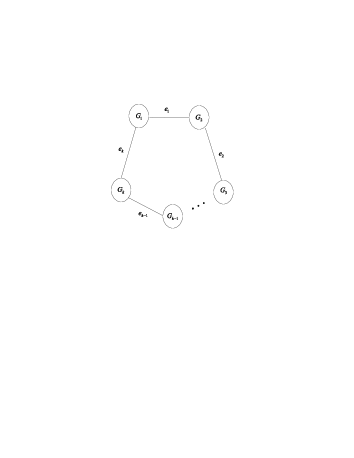
Fig. 4: $S=\{e_{1},e_{2},\cdots,e_{k}\}$ and $G-S=G_{1}\cup G_{2}\cup\cdots\cup G_{k}$ and each $G_{i}$ ($i=1,2,\cdots,k$) is connected.

Proof. We first prove that if $k(G-S)=|S|$, then all edges of $S$ occur on a cycle of $G$ as shown in Fig. 4. It holds when $|S|=2$ and now we suppose $|S|\geq 3$ and $f\in S$. By $k(G-S)=|S|$ we have $k(G-S+f)=|S-f|$ and $f$ is a bridge of $G-S+f$. By induction hypothesis we have $S-f$ occur on a cycle of $G$. Suppose that $G$ becomes $G_{1},G_{2},\cdots,G_{|S-f|}$ when $S-f$ deleted. Then $f$ belongs to some $G_{i}$ and is also a bridge of $G_{i}$. Hence, all edges of $S$ occur on a cycle of $G$.

It is clear that if all edges of $S$ occur on a cycle of $G$ as shown in Fig. 4, then $S$ is a pairwise-disconnecting set.

Finally we prove that if $S$ is pairwise-disconnecting set, then $k(G-S)=|S|$. It holds when $|S|=2$ and now we suppose $|S|\geq 3$ and $f\in S$. Then $S-f$ is also a pairwise-disconnecting set. By induction hypothesis we have $k(G-S+f)=|S-f|$. Let $g\in S-f$. Then $\{f,g\}$ is a 2-edge cut of $G$. Hence, $f$ is a bridge of $G-g$ and also a bridge of $G-S+f$. Therefore, we have $k(G-S)=k(G-S+f)+1=|S-f|+1=|S|$. $\Box$

A pairwise-disconnecting set $S_{M}$ is said to be maximal if no pairwise-disconnecting set contains it as a proper subset.

Proposition 4.3

Let $G$ be a connected bridgeless graph. For any given pairwise-disconnecting set $S$ of $G$, there exists a unique maximal pairwise-disconnecting set $S_{M}$ of $G$ containing $S$.

Proof. The existence follows from the definition of pairwise-disconnecting sets directly. To prove the uniqueness, we suppose that there are two distinct maximal pairwise-disconnecting sets $S_{M}^{1}$ and $S_{M}^{2}$ of $G$ such that $S\subset S_{M}^{i}$ ($i=1,2$). Let $e,f\in S$ and $g\in S_{M}^{2}-S_{M}^{1}$. Then $\{e,f\}$ is a 2-edge cut of $G$ and suppose that $G-e-f=G_{1}\cup G_{2}$. Without loss of generality we suppose that $g\in E(G_{2})$. Since $e,f,g\in S_{M}^{2}$ we obtain that $\{e,g\}$ is a 2-edge cut of $G$, which implies that $g$ must be a bridge of $G_{2}$. We suppose that $G_{2}-g=G_{2}^{\prime}\cup G_{2}^{\prime\prime}$. See Fig. 5 (a). Let $h\in S_{M}^{1}-e-f$. We shall show that $\{h,g\}$ is a 2-edge cut of $G$. Since $e,f,h\in S_{M}^{1}$ we obtain that $\{e,h\}$ is a 2-edge cut of $G$, which implies that $h$ must be a bridge of $G_{1}$ or $G_{2}$. There are two cases.

Case 1. $h$ is a bridge of $G_{1}$. Suppose that $G_{1}-h=G_{1}^{\prime}\cup G_{1}^{\prime\prime}$, then $G-g-h$ is disconnected as shown in Fig. 5 (b).

Case 2. $h$ is a bridge of $G_{2}$. Without loss of generality, we suppose that $h\in G_{2}^{\prime}$, then $h$ is also a bridge of $G_{2}^{\prime}$. Suppose that $G_{2}^{\prime}-h=G_{21}^{\prime}\cup G_{22}^{\prime}$, then $G-g-h$ is also disconnected as shown in Fig. 5 (c).

Hence, $S_{M}^{1}\cup\{g\}$ is a pairwise-disconnecting set, which contradicts the maximality of $S_{M}^{1}$. $\Box$

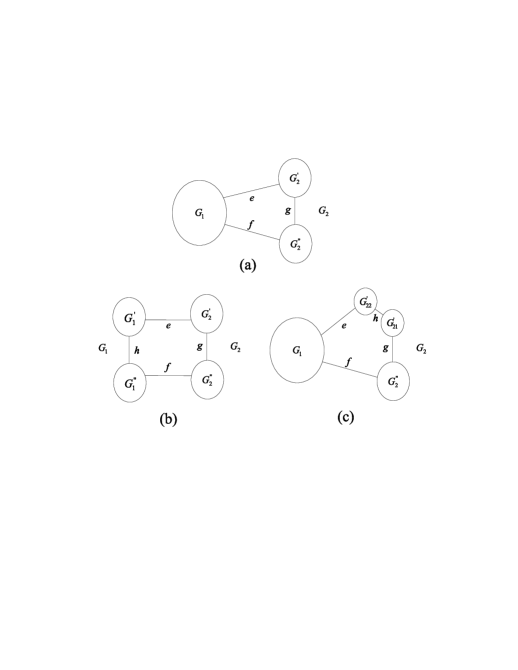
Fig. 5: The proof of Proposition 4.3.

Now we are in a position to prove a ’dual’ result of Lemma 4.1.

Lemma 4.4

Let $G=(V,E)$ be a connected bridgeless graph. Let the Tutte polynomial evaluation

$$T_{G}(-t,-t^{-1})=a_{n}t^{n}+a_{n+1}t^{n+1}+\cdots+a_{m-1}t^{m-1}+a_{m}t^{m}$$

with $a_{n}\neq 0,a_{m}\neq 0$ and $n\leq m$. Then $n=-|E|+|V|-1$ and

1. $a_{n}=(-1)^{|E|-|V|+1}$.

2. $a_{n+1}=(-1)^{|E|-|V|+1}(-|V|+1+\sum_{S_{M}}(|S_{M}|-1))$, where $S_{M}$ is a maximal pairwise-disconnecting set and the summation is over all maximal pairwise-disconnecting sets.

Proof. Recall that

$$T_{G}(-t,-t^{-1}) = \sum_{F\subseteq E}(-t-1)^{k(F)-1}(-t^{-1}-1)^{|F|-|V|+k(F)}$$

$$= \sum_{F\subseteq E}(-1)^{|F|-|V|+1}(1+t)^{k(F)-1}(t^{-1}+1)^{|F|-|V|+k(F)}.$$

It is clear that $k(F)-1\geq 0$. Thus we obtain

$$(1+t)^{k(F)-1}=1+(k(F)-1)t+\left(\begin{array}[]{c}k(F)-1\\ 2\end{array}\right)t^{2}+\cdots.$$

Since $|F|-|V|+k(F)$ is the nullity of the subgraph $(V,F)$ of $G=(V,E)$, $0\leq|F|-|V|+k(F)\leq|E|-|V|+1$. $(t^{-1}+1)^{|F|-|V|+k(F)}$ now can be expressed as

$$t^{-({|F|-|V|+k(F)})}+({|F|-|V|+k(F)})t^{-(|F|-|V|+k(F)-1)}+$$

$$\left(\begin{array}[]{c}|F|-|V|+k(F)\\ 2\end{array}\right)t^{-(|F|-|V|+k(F)-2)}+\cdots.$$

Note that $G$ is connected and bridgeless, we have $|F|-|V|+k(F)=|E|-|V|+1$ if and only if $F=E$. Hence, we have $n=-|E|+|V|-1$ and $a_{n}=(-1)^{|E|-|V|+1}$. Furthermore, $|F|-|V|+k(F)=|E|-|V|$ if and only if $F=E-e$ for $e\in E$ or, by Proposition 4.2 $F=E-S$, where $S$ is a pairwise-disconnecting set of $G$. Thus,

$$a_{n+1} = (-1)^{|E|-|V|+1}(|E|-|V|+1)+(-1)^{|E|-|V|}|E|+\sum_{E-S}(-1)^{|E-S|-|V|+1}$$

$$= (-1)^{|E|-|V|+1}(-|V|+1)+\sum_{E-S_{M}}\sum_{S\subset S_{M}}(-1)^{|E-S|-|V|+1}$$

(By Proposition 4.3)

$$= (-1)^{|E|-|V|+1}(-|V|+1+\sum_{S_{M}}(|S_{M}|-1)).$$

$\Box$

Remark 4.5

Results of Lemmas 4.1 and 4.4 are dual in the sense that (maximal) multiple edge corresponds to (maximal) pairwise-disconnecting set by taking the dual when they are both plane graphs.

Theorem 4.6

Let $G$ be a connected bridgeless and loopless positive graph. Then the highest and lowest degrees of $Q[G]$ are $3|E|-2|V|+2$ and $-|E|-2|V|+2$, respectively. Furthermore,

1. the coefficient of the term with the highest degree is $(-1)^{|E|-|V|+1}$,

2. the coefficient of the term with the lowest degree is $(-1)^{|V|-1}$,

3. the coefficient of the term with the second-highest degree is $(-1)^{|E|-|V|+1}(-|V|+1+\sum_{S_{M}}(|S_{M}|-1))$,

4. the coefficient of the term with the second-lowest degree is $(-1)^{|V|-1}(|V|-1-|E|+\sum_{I_{M}}(|I_{M}|-1))$.

Proof. It follows from Lemmas 2.7, 4.1 and 4.4. $\Box$

Remark 4.7

Theorem 4.6 (1) and (2) are the generalization of Lemma 2.3 from planar graphs to all abstract (not necessarily planar) graphs. It is not difficult to verify that when $G$ is a plane graph, Theorem 4.6 (1) and (2) coincide with Lemma 2.3.

5 The proof of Theorem 1.2

To prove Theorem 1.2, we first need to further study the properties of maximal pairwise-disconnecting sets. Let $G$ be a connected bridgeless graph and $S$ be a pairwise-disconnecting set. For any $e\in S$, we define $S_{M}(e)$ to be the union of $\{e\}$ and the set of all bridges of $G-e$.

Proposition 5.1

For any $e,f\in S$, $S_{M}(e)=S_{M}(f)$ and it is exactly the unique maximal pairwise-disconnecting set containing $S$.

Proof. It suffices for us to prove that $S_{M}(e)\subset S_{M}(f)$. It is clear that $e\in S_{M}(f)$ since $e,f\in S$ implying that $\{e,f\}$ constitutes a 2-edge cut of $G$. For any $g\in S_{M}(e)$ and $g\neq e$, $g$ is a bridge of $G-e$. Recall that $\{e,f\}$ is a 2-edge cut of $G$ and suppose that $G-e-f=G_{1}\cup G_{2}$ and $g\in E(G_{2})$. $g$ is a bridge of $G-e$ implies that $g$ is a bridge of $G_{2}$, and is also a bridge of $G-f$. Hence, $g\in S_{M}(f)$ and we proved that $S_{M}(e)\subset S_{M}(f)$.

It is clear that $S\subset S_{M}(e)$. Now we prove that $S_{M}(e)$ is a maximal pairwise-disconnecting set. According to the definition of $S_{M}(e)$ we know that $k(G-S_{M}(e))=|S_{M}(e)|$. By Proposition 4.2, we have $S_{M}(e)$ is a pairwise-disconnecting set. To prove the maximality of $S_{M}(e)$, we suppose that $g\notin S_{M}(e)$ and $\{g\}\cup S_{M}(e)$ is a pairwise-disconnecting set. Then $\{e,g\}$ is a 2-edge cut of $G$ and $g$ is a bridge of $G-e$, contradicting $g\notin S_{M}(e)$. $\Box$

Proposition 5.2

Any two distinct maximal pairwise-disconnecting sets of a connected bridgeless graph are disjoint.

Proof. Suppose that $S_{M}^{1}$ and $S_{M}^{2}$ are two distinct maximal pairwise-disconnecting sets of a connected bridgeless graph $G$ and $e\in S_{M}^{1}\cap S_{M}^{2}$. By Proposition 5.1, $S_{M}^{i}$ ($i=1,2$) will both be the union of $\{e\}$ and the set of all bridges of $G-e$ and hence, will be equal, a contradiction. $\Box$

Proposition 5.3

A pairwise-disconnecting set $S=\{e_{1},e_{2},\cdots,e_{k}\}$ of a connected bridgeless graph $G$ as shown in Fig. 4 is maximal if and only if each $G_{i}$ ($i=1,2,\cdots,k$) is bridgeless.

Proof. It is obvious. $\Box$

Now we are in a position to prove Theorem 1.2.

Proof. If $\tilde{L}$ is not connected, then the $<$ of Eq. (4) holds. From the proof of Theorem 1.1, we know that $c(\tilde{L})=c(L)-2$ if and only if the Case 2a happens.

If $\tilde{L}$ is connected, then the $=$ of Eq. (4) holds. Let $a_{2}$ (resp. $b_{2}$) be the coefficient of the degree $e(G)+2f(G)-4$ (resp. $-e(G)-2v(G)+8$) in $Q[\tilde{G}]$. From the proof of Theorem 1.1, the equality of Theorem 1.1 holds if and only if $a_{2}\neq 0$ and $b_{2}\neq 0$. There are two cases.

Case 1. $G^{\prime\prime}=G/e$ is loopless.

Note that $G^{\prime\prime}$ is loopless means that $\mu(e)=1$. By Eq. (5) and Theorem 4.6, we obtain that

$$a_{2} = (-1)^{|E|-|V|+1}(-|V|+1+\sum_{S_{M}}(|S_{M}|-1))+(-1)^{|E^{\prime\prime}|-|V^{\prime\prime}|+1}-$$

$$(-1)^{|E^{\prime\prime}|-|V^{\prime\prime}|+1}(-|V^{\prime\prime}|+1+\sum_{S_{M}^{\prime\prime}}(|S_{M}^{\prime\prime}|-1))$$

$$= (-1)^{|E|-|V|+1}(-|V|+1+\sum_{S_{M}}(|S_{M}|-1)+1+|V^{\prime\prime}|-1-\sum_{S_{M}^{\prime\prime}}(|S_{M}^{\prime\prime}|-1))$$

$$= (-1)^{|E|-|V|+1}(\sum_{S_{M}}(|S_{M}|-1)-\sum_{S_{M}^{\prime\prime}}(|S_{M}^{\prime\prime}|-1)).$$

Maximal pairwise-disconnecting sets of $G$ can be divided into two classes: those containing the edge $e$ and those not containing the edge $e$. Let $S_{M}$ be a maximal pairwise-disconnecting set of $G$. By Proposition 5.3, we obtain that $G-S_{M}=G_{1}\cup G_{2}\cup\cdots\cup G_{|S_{M}|}$ and each $G_{i}$ ($i=1,2,\cdots,|S_{M}|$) is bridgeless. If $e\in S_{M}$, suppose that $e$ connects $G_{i}$ to $G_{i+1}$ for some $i$. Since the one-point join of $G_{i}$ and $G_{i+1}$ is bridgeless, by Proposition 5.3 we have $S_{M}-e$ is a maximal pairwise-disconnecting set of $G^{\prime\prime}$. If $e\notin S_{M}$, suppose $e\in E(G_{i})$ for some $i$. Since $G_{i}/e$ is bridgeless, we have $S_{M}$ is also a maximal pairwise-disconnecting set of $G^{\prime\prime}$.

Conversely, let $S_{M}^{\prime\prime}$ be a maximal pairwise-disconnecting set of $G^{\prime\prime}$. By Proposition 5.3, we obtain that $G^{\prime\prime}-S_{M}^{\prime\prime}=G_{1}^{\prime\prime}\cup G_{2}^{\prime\prime}\cup\cdots\cup G_{|S_{M}^{\prime\prime}|}^{\prime\prime}$ and each $G_{i}^{\prime\prime}$ ($i=1,2,\cdots,|S_{M}^{\prime\prime}|$) is bridgeless. Note that the two end-vertices $u$ and $v$ of the edge $e$ of $G$ is identified to become one vertex, say $u^{\prime\prime}$, in $G^{\prime\prime}$. Suppose that $u^{\prime\prime}\in V(G_{i}^{\prime\prime})$ for some $i$ and $G-S_{M}^{\prime\prime}=G_{1}^{\prime\prime}\cup\cdots\cup G_{i-1}^{\prime\prime}\cup G_{i}\cup G_{i+1}^{\prime\prime}\cup\cdots\cup G_{|S_{M}^{\prime\prime}|}^{\prime\prime}$. Then $G_{i}^{\prime\prime}=G_{i}/e$. If $e$ is not a bridge of $G_{i}$, then $S_{M}^{\prime\prime}$ is a maximal pairwise-disconnecting set of $G$. If $e$ is a bridge of $G_{i}$, then $S_{M}^{\prime\prime}\cup\{e\}$ will be a maximal pairwise-disconnecting set of $G$. Suppose that $G$ has exactly $k$ maximal pairwise-disconnecting sets containing the edge $e$. Then

$$a_{2} = (-1)^{|E|-|V|+1}k.$$

Furthermore, by Proposition 5.2, $k=0$ or $1$. Thus $a_{2}\neq 0$ iff $G$ has (a unique) maximal pairwise-disconnecting set containing the edge $e$ iff $G-e$ has bridges.

Similarly, we have

$$b_{2} = (-1)^{|V|-1}(|V|-1-|E_{s}|)-(-1)^{|V^{\prime\prime}|-1}+(-1)^{|V^{\prime\prime}|-1}(|V^{\prime\prime}|-1-|E_{s}^{\prime\prime}|)$$

$$= (-1)^{|V|-1}(|V|-1-|E_{s}|+1-|V^{\prime\prime}|+1+|E_{s}^{\prime\prime}|)$$

$$= (-1)^{|V|-1}(|E_{s}^{\prime\prime}|+2-|E_{s}|).$$

It is not difficult to see that $|E_{s}|=|E_{s}^{\prime\prime}|+1+|N(u)\cap N(v)|$. So $b_{2}\neq 0$ iff $|N(u)\cap N(v)|\neq 1$.

Moreover, $G-e$ has bridges imply that $|N(u)\cap N(v)|\leq 1$ (see Fig. 4). Thus $a_{2}\neq 0$ and $b_{2}\neq 0$ if and only if $G-e$ has bridges and $N(u)\cap N(v)=\emptyset.$

Case 2. $G^{\prime\prime}$ has loops.

This means $\mu(e)\geq 2$. For any edge $f\in E(G)$, which is parallel to $e$, if $G-e-f$ is disconnected, then $\tilde{L}$ will be a split link. Hence $G-e-f$ is connected. Recall that $\tilde{G}$ corresponding to $\tilde{L}$ is obtained from $G$ by changing the sign of $e$ from $+$ and $-$. Note that $e$ and $f$ will cancel each other in $\tilde{G}$ by the second Reidemeister move and $\tilde{G}-e-f=G-e-f$ is positive and loopless, we have $c(\tilde{L})=c(L)-2$ if and only if $G-e-f$ is connected and bridgeless. $\Box$

6 Examples and further discussions

In this section, we first provide an example to illustrate Theorem 1.2. It is well known that rational knots are alternating and by changing a crossing of a rational knot we still obtain a rational knot.

Example 6.1

The rational knot $10_{14}$ (see [1] P. 47) (the dashed curve) and its corresponding graph $G$ (the thick curve) are shown in Fig. 6. For $i=1,2,3,4$, $\mu(i)=1$, $G-i$ has bridges, the two end-vertices of $i$ have no common neighbors. For $i=5,6$, $\mu(i)=2$, $G-\{5,6\}$ is connected and bridgeless. For $i=7,8$, $\mu(i)=1$, $G-i$ has no bridges. For $i=9,10$, $\mu(i)=1$, $G-i$ has bridges, the two end-vertices of $i$ have one common neighbor. Hence the crossing number is reduced exactly by 2 after changing the crossing $i$ for $i=1,2,3,4,5,6$ and reduced by 3 or more after changing the crossing $i$ for $i=7,8,9,10$.

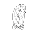
Fig. 6: The knot $10_{14}$ (the dashed curve) and its corresponding graph (the thick curve).

In the Dale Rolfsen’s Knot table, if an alternating knot diagram corresponds to a negative plane graph, we shall take its mirror image to obtain a positive plane graph. Among alternating knots whose crossing number is less than 10, there are only 11 knot diagrams whose corresponding positive plane graphs satisfy conditions of Corollary 1.3, and they are $5_{1}$,$7_{1}$,$7_{3}$,$8_{3}$,$8_{5}$,$9_{1}$,$9_{3}$,$9_{4}$,$9_{9}$,$9_{10}$,$9_{35}$. There are only 5 knot diagrams whose corresponding positive plane graphs satisfy conditions of Corollary 1.4, and they are $5_{1}$,$7_{1}$,$8_{5}$,$9_{1}$,$9_{35}$.

Moreover, in graph theory, it is easy to judge whether an edge is a bridge or not. As for the condition $N(u)\cap N(v)=\emptyset$, under conditions $\mu(e)=1$ and $G-e$ has bridges, there are only two types of graphs with $N(u)\cap N(v)\neq\emptyset$ as shown in Fig. 7.

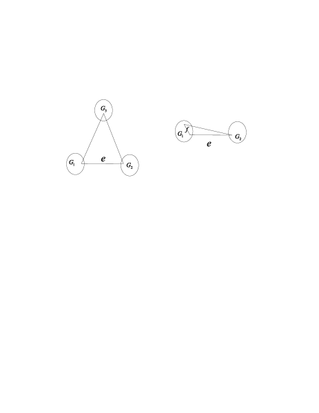
Fig. 7: Two types of graphs with $\mu(e)=1$, $G-e$ has bridges and $N(u)\cap N(v)\neq\emptyset$. In both types $G_{i}$ is bridgeless and in the second type $f\in E(G_{1})$.

Finally, although sufficient and necessary conditions of Theorem 1.2 and two corollaries are very simple, applications of Theorem 1.2 or its two corollaries are still very limited since the properties, non-split and alternating of $\tilde{L}$, have not been converted to conditions of $G$ (and the edge $e$). We pose the following two problems for further study.

Problem 1. Let $G$ be a positive plane graph, $e$ be an edge of $G$. Let $\tilde{L}$ be the link whose diagram corresponds to the plane graph obtained from $G$ by changing the sign of $e$ from $+$ to $-$. We ask which conditions should be satisfied by $G$ and $e$ to guarantee that the link $\tilde{L}$ is non-split?

We note that Problem 1 appears in Page 143 of [1] as an unsolved question.

Problem 2. Let $G$ be a positive plane graph, $e$ be an edge of $G$. Let $\tilde{L}$ be the link whose diagram corresponds to the plane graph obtained from $G$ by changing the sign of $e$ from $+$ to $-$. We ask which conditions should be satisfied by $G$ and $e$ to guarantee that the link $\tilde{L}$ is alternating?

Acknowledgements

This paper was supported by NSFC Grant No. 10831001 and Grant No. 11271307. We thank the referees for their suggestions.

References

- [1] C. C. Adams, The knot book, American Mathematical Society, 2004.
- [2] T. Albertson, The twist numbers of graphs and the Tutte polynomial, see http://www.math.csusb.edu/reu/ta05.pdf.
- [3] B. Bollobás, Modern Graph Theory, Springer, Berlin, 1998.
- [4] J. A. Bondy, U. S. R. Murty, Graph theory and its applications, The Macmillan press ltd, 1976.
- [5] G. Chaty, M. Chein, Minimally 2-edge connected graphs, J. Graph Theory 3(1) (1979) 15-22.
- [6] Y. Diao, C. Ernst, A. Stasiak, A partial ordering of knots and links through diagramtic unknotting, J. Knot Theory Ramifications 18(4) (2009) 505-522.
- [7] T. Endo, T. Itoh, K. Taniyama, A graph-theoretic approach to a partial order of knots and links, Topology Appl. 157 (2010) 1002-1010.
- [8] D. Eppstein, On the parity of graph spanning tree numbers, Tech. Report 96-14, Univ. of California, Irvine, Dept. of Information and Computer Science, 1996.
- [9] C. Godsil, G. Royle, Algebraic graph theory, Springer, 2004.
- [10] V. F. R. Jones, A polynomial invariant for knots via von Neumann algebras, Bull. Amer. Math. Soc. 12 (1985) 103-111.
- [11] L. H. Kauffman, State models and the Jones polynomial, Topology 26 (1987) no. 3, 395-407.
- [12] L. H. Kauffman, New invariants in the theory of knots, Amer. Math. Monthly 95 (1988) 195-242.
- [13] L. H. Kauffman, A Tutte polynomial for signed graphs, Discrete Appl. Math. 25 (1989) 105-127.
- [14] O. Dasbach, X.-S. Lin, A volumish theorem for the Jones polynomial of alternating knots, Pacific J. Math. 231 (2007) no. 2, 279-291.
- [15] K. Murasugi, Knot theory and its applications, Birkhauser, 1996.
- [16] K. Murasugi, Jones polynomials and classical conjectures in knot theory, Topology 26 (1987) no. 2, 187-194.
- [17] H. Shank, The theory of left-right paths, in: Combinatorial Mathematics III, Lecture Notes in Math., Vol. 452, Springer, Berlin, 1975, pp. 42-54.
- [18] K. Taniyama, A partial order of knots, Tokyo J. Math. 12 (1989) 205-229.
- [19] M. B. Thistlethwaite, A spanning tree expansion of the Jones polynomial, Topology 26 (1987) no. 3, 297-309.
- [20] W. T. Tutte, A contribution to the theory of chromatic polynomials, Canad. J. Math. 6 (1954) 80-91.
- [21] L. Wu, S. Shao, S. Liu, F. Lei, Effect of a crossing change on crossing number, arXiv:1103.4695v1 [math.GT] 24 Mar 2011.
- [22] B. Zhu, Some properties of minimal 2-edge connected graph, Acta Math. Sin. 24 (1981) 436-443.