xTRAM: Estimating equilibrium expectations from time-correlated simulation data at multiple thermodynamic states

Abstract

Computing the equilibrium properties of complex systems, such as free energy differences, is often hampered by rare events in the dynamics. Enhanced sampling methods may be used in order to speed up sampling by, for example, using high temperatures, as in parallel tempering, or simulating with a biasing potential such as in the case of umbrella sampling. The equilibrium properties of the thermodynamic state of interest (e.g., lowest temperature or unbiased potential) can be computed using reweighting estimators such as the weighted histogram analysis method or the multistate Bennett acceptance ratio (MBAR). weighted histogram analysis method and MBAR produce unbiased estimates, the simulation samples from the global equilibria at their respective thermodynamic state–a requirement that can be prohibitively expensive for some simulations such as a large parallel tempering ensemble of an explicitly solvated biomolecule. Here, we introduce the transition-based reweighting analysis method (TRAM)–a class of estimators that exploit ideas from Markov modeling and only require the simulation data to be in local equilibrium within subsets of the configuration space. We formulate the expanded TRAM (xTRAM) estimator that is shown to be asymptotically unbiased and a generalization of MBAR. Using four exemplary systems of varying complexity, we demonstrate the improved convergence (ranging from a twofold improvement to several orders of magnitude) of xTRAM in comparison to a direct counting estimator and MBAR, with respect to the invested simulation effort. Lastly, we introduce a random-swapping simulation protocol that can be used with xTRAM, gaining orders-of-magnitude advantages over simulation protocols that require the constraint of sampling from a global equilibrium.

I Introduction

The successful prediction of equilibrium behavior of complex systems is of critical importance in computational physics. Often, rare events in the system’s dynamics make such estimates through direct simulations impractical. For this reason, the past 20 years have seen vast progress in computational techniques used for efficient sampling of rare events systems with complex energy landscapes. These developments were in particular driven by the study of systems such as spin glasses Katzberger et al. (2001); Bittner and Janke (2006), quantum frustrated spin systems Melko (2007); de Candia and Coniglio (2001), QCD Ilgenfritz et al. (2002); Burgio et al. (2007); Joo et al. (1999) and molecular dynamics (MD) of biomolecules Hansmann (1997); Sugita and Okamoto (1999).

Commonly used approaches are generalized ensemble methods such as simulated tempering (ST) Marinari and Parisi (1992), parallel tempering (PT) Hukushima and Nemoto (1996); Hansmann (1997); Sugita and Okamoto (1999) or replica exchange molecular dynamics (REMD) Greyer (1991). Generalized ensemble methods can greatly improve the convergence over direct simulation for systems with high energy barriers but relatively few degrees of freedom Sindhikara et al. (2010); Park (2008); Abraham and Gready (2008). The speed of convergence depends on the overlap of energy distributions between adjacent temperatures, and thus efforts have been made in choosing optimal temperature distributions Zheng et al. (2007); Rosta and Hummer (2009, 2010); Hansmann (1997). Unfortunately, the number of replicas needed to fill the relevant range of temperatures, increases with the number of degrees of freedom of the system, and produce expensive computational requirements for many-body systems such as explicitly solvated molecules.

Once a multi-ensemble simulation was generated, there are different estimator options that can be used for the analysis of the simulation data in order to extract information such as free energy differences between conformations of interest. The simplest estimator is to bin the simulation data (in a single order parameter or using clusters of a high-dimensional parameter space) at the temperature of interest and count the number of occurrences of each of the discrete states. We will refer to this estimation method as the direct counting estimator. An improvement over direct counting of single temperature histograms, is the weighted histogram analysis method (WHAM) Ferrenberg and Swendsen (1989); Kumar et al. (1992). WHAM makes use of data from all simulated temperatures by reweighting them to the target temperature via the Boltzmann density. The traditional WHAM formulation in multi-temperature ensembles requires to discretize the system’s potential energy in order to formulate a reweighting factor for each energy bin Gallicchio et al. (2005). A formulation of WHAM that avoids the potential-energy binning is given in Souaille and Roux (2001). Ref. Shirts and Chodera (2008) generalizes this concept and derives the multistate Bennett acceptance ratio (MBAR) that produces statistically optimal estimates of equilibrium properties given a set of equilibrium data.

All of the above estimators assume that the data are sampled from global equilibrium, i.e. simulations at all temperatures have entirely decorrelated from their starting configurations. This often requires discarding large amounts of data for producing unbiased estimates. This can lead to very long simulation times in order to obtain an uncorrelated sample.

Here, we combine ideas from reweighting estimators Bennett (1976) and Markov model theory Schütte et al. (1999); Singhal and Pande (2005); Chodera et al. (2006); Noé et al. (2007); Chodera et al. (2007); Prinz et al. (2011) in order to derive a transition-based reweighting analysis method (TRAM) for estimating equilibrium properties from simulation data at multiple thermodynamic states. TRAM differs from established reweighting estimators such as direct counting, WHAM or MBAR, in that it uses conditional transition probabilities between the discrete states or bins and therefore does not require the underlying data to be in global equilibrium. Thus, TRAM can achieve unbiased equilibrium estimates for data that is not yet in global equilibrium, allowing accurate estimates to be obtained with sometimes orders of magnitude smaller simulation times compared to established estimators.

Markov models are usually used for predicting long term kinetics from short time simulation data Noé et al. (2009), requiring the use of sufficiently long lag times when computing the conditional transition probabilities Prinz et al. (2011). Therefore, extracting kinetics from generalized ensemble simulations is difficult. If desired, one either has to limit the lag time to the short contiguous simulations times Sriraman et al. (2005), or one has to reweight entire trajectories Chodera et al. (2011); Prinz et al. (2011). However, a transition matrix can be used to estimate the equilibrium distribution of a system without requiring log lag times Prinz et al. (2011). At a given temperature $T^{I}$, the corresponding transition matrix $\mathbf{P}^{I}$ provides an estimate of the equilibrium distribution $\boldsymbol{\pi}^{I}$ as its dominant eigenvector. However, in order to exploit the existence of high temperatures in the simulation, an estimator must be constructed that connects the different temperatures in a rigorous way. This leads to the proposal of a transition-based reweighting analysis method (TRAM).

TRAM can also be employed to get estimates from multiple biased simulations, such as umbrella sampling Torrie and Valleau (1977) or metadynamics Laio and Parrinello (2002), although we will here focus on applications using multi-temperature ensembles. In general, by TRAM we refer to a class of estimators with the following behavior:

1. Given simulations at different thermodynamic states $I=1,...,m$ (temperatures, bias potentials, …), and a configuration-space discretization into discrete states $i=1,...,n$ (binning along an order parameter or clustering of a high-dimensional space), harvest the following statistics:

   1. At each thermodynamic state $I$, the number of transitions $c_{ij}^{I}$ observed between configuration states $i$, $j$ at a time lag $\tau$ (here usually the data storage interval).

   2. For each sample $\mathbf{x}$ along the trajectory, with thermodynamic state $I$ and configuration state $i$ the probability weight $\mu^{J}(\mathbf{x})$ this sample $\mathbf{x}$ would be attributed in all other thermodynamic states $J=1,...,m$, $\mu^{J}(\mathbf{x})$.

2. Compute an optimal estimate of the equilibrium probability $\pi_{i}^{I}$ for all configuration states $i$ at all thermodynamic states $I$.

With the help of the equilibrium probabilities $\pi_{i}^{I}$, other equilibrium expectations can be computed. Due to property (1a), TRAM is a “transition-based” estimator rather than a histogram method. Due to property (1b), TRAM is also a “reweighting” estimator. TRAM estimators do not depend on actual temperature-transitions in the generalized ensemble. Rather, all configurations visited during the simulation will be used to estimate transition probabilities between thermodynamic states.

Different implementations of TRAM estimators and formulations of their optimality may be possible, we therefore consider TRAM to be a class of estimators rather than a unique method. In this paper we propose a TRAM estimator which formally constructs an expanded $(mn\times mn)$ transition matrix in the joint space of all $m$ thermodynamic states and $n$ configuration states. Therefore, the present estimator is called expanded TRAM (xTRAM). The stationary eigenvector of the xTRAM transition matrix contains the equilibrium probabilities at all thermodynamic states.

While simulation protocols such as ST, PT and REMD require a strong overlap of energy distributions between neighboring temperatures to be efficient for sampling, this is much less relevant for the usefulness of TRAM estimators as the reweighting factors are useful information even when the transition probabilities between thermodynamic states are small. It is thus tempting to design new simulation protocols that achieve more efficient sampling by sacrificing the asymptotic global equilibrium property achieved by ST, PT and REMD, but can still yield unbiased estimates of equilibrium probabilities when used in conjunction with TRAM estimators. In this paper we make a first attempt to this end and propose the random swapping (RS) simulation method. RS achieves rapid mixing between a set of replicas that would be too sparsely distributed for ST, PT or REMD because it exchanges without Metropolis-Hastings acceptance step. The associated violation of global equilibrium can be approximately recovered by xTRAM because local equilibrium is guaranteed by adjusting lag times $\tau$ during the estimation accordingly.

xTRAM is shown to be asymptotically unbiased. Moreover, we show that xTRAM is a generalization of MBAR which converge to identical estimators for the free energy differences between thermodynamic states in the limit of global equilibrium, and to identical estimators for general equilibrium expectations in the limit of global equilibrium and large statistics.

Using xTRAM and in particular with the combination of xTRAM and RS, estimates of equilibrium properties of complex dynamical systems can be obtained with orders of magnitude fewer simulation data than that required by conventional estimators. We illustrate the performance of TRAM, MBAR and direct counting on two bistable model potentials and two explicitly solvated peptides simulated with Molecular Dynamics simulations.

II Theory and Methods

II.1 Scope

A configuration $\mathbf{x}$ is a point in configuration space $\Omega$ containing all quantities characterizing the instantaneous state of the system, such as particle positions or spins, system volume (in constant-pressure ensembles), and particle numbers (in ensembles of constant chemical potential).

We consider a set of simulation trajectories, each sampling from $\Omega$, at a given thermodynamic state $I$. A thermodynamic state, here denoted as capital superscript letters $I$, $J$, $K$, is characterized by its thermodynamic variables, such as temperature, pressure or chemical potential. The dynamics are assumed to fulfill microscopic detailed balance at their respective thermodynamic states.

We consider $\Omega$ to be partitioned into subsets $S_{i}$ such that $\Omega=\bigcup_{i=1}^{n}S_{i}$. We will subsequently refer to subsets $S_{i}$ as configuration states and index them by small subscript letters $i,j,k$. This discretization serves to distinguish the states that are relevant to the analyst. As such it may consist of a fine discretization of an order parameter of interest (e.g. magnetization in an Ising model), or a Voronoi partition obtained from clustering molecular dynamics data, as is frequently used for the construction of Markov models.

TRAM estimators will use statistics from transitions among configuration states, but also exploit the fact that the statistical weight of a configuration $\mathbf{x}$ can be reweighted between thermodynamic states. Consider the following two examples:

1. In PT or REMD simulations, the weighting occurs through the different temperatures: Given a configuration $\mathbf{x}$ with potential energy $U(\mathbf{x})$, the statistical weight at temperature $T^{I}$ is proportional to $\mathrm{e}^{-u^{I}(\mathbf{x})}$ using the reduced potential energy

   $$u^{I}(\mathbf{x})=\frac{U(\mathbf{x})}{k_{B}T^{I}},$$ (1)

   with Boltzmann constant $k_{B}$.

2. When the simulation setup contains multiple biased simulations, such as in umbrella sampling or metadynamics, there is usually a unique temperature $T$, but different potentials $U^{I}(\mathbf{x})=U(\mathbf{x})+B^{I}(\mathbf{x})$ are employed where $B^{I}(\mathbf{x})$ is the $I$th bias potential. Then the statistical weights in each of these potentials is given by $\mathrm{e}^{-u^{I}(\mathbf{x})}$ with:

   $$u^{I}(\mathbf{x})=\frac{U(\mathbf{x})+B^{I}(\mathbf{x})}{k_{B}T}.$$ (2)

We generalize this concept following the example of Shirts and Chodera (2008). In a thermodynamic state $I$, defined by a particular combination of the potential energy function $U^{I}$, pressure $p^{I}$, chemical potentials $\mu_{s}^{I}$ of chemical species $s$ and temperature $T^{I}$, our system has a reduced potential defined by:

$$u^{I}(\mathbf{x})=\frac{U^{I}(\mathbf{x})+p^{I}V(\mathbf{x})+\sum_{s}\mu_{s}^{I}N_{s}(\mathbf{x})}{k_{B}T^{I}}.$$ (3)

Here, $V(\mathbf{x})$ is the volume of the system in configuration $\mathbf{x}$ and $N_{s}(\mathbf{x})$ counts the particle numbers of species $s$ at configuration $\mathbf{x}$. The probability density of configuration $\mathbf{x}$ can, for any arbitrarily chosen thermodynamic state, be expressed as:

$$\rho^{I}(\mathbf{x})=\frac{1}{Z^{I}}e^{-u^{I}(\mathbf{x})},$$ (4)

where $Z^{I}$ is the partition function of thermodynamic state $I$:

$$Z^{I}=\int_{\Omega}d\mathbf{x}\>e^{-u^{I}(\mathbf{x})}.$$ (5)

The partition function of configuration state $i$ at thermodynamic state $I$ is:

$$Z_{i}^{I}=\int_{S_{i}}d\mathbf{x}\>e^{-u^{I}(\mathbf{x})}.$$ (6)

II.2 Aims

Next, we will define the quantities we would like to estimate using TRAM. The reduced free energy of thermodynamic state $I$, $f^{I}$, and the reduced free energy of configuration state $i$ at thermodynamic state $I$,$f_{i}^{I}$, here termed the configuration free energy are defined as:

$$f^{I} :=-\ln Z^{I}$$ (7)

$$f_{i}^{I} :=-\ln Z_{i}^{I}.$$ (8)

The equilibrium probability of configuration state $i$, given that the system is at thermodynamic state $I$ is:

$$\pi_{i}^{I}:=\frac{Z_{i}^{I}}{Z^{I}}=\mathrm{e}^{f^{I}-f_{i}^{I}}.$$ (9)

Finally, we are interested in computing expectation values of arbitrary functions of configuration state $A(\mathbf{x})$:

$$\langle A\rangle_{I}=\int_{\Omega}d\mathbf{x}\>\rho^{I}(\mathbf{x})\>A(\mathbf{x}).$$ (10)

The multistate Bennett acceptance ratio estimator Shirts and Chodera (2008) can provide statistically optimal estimates for quantities (7)-(10) when all samples $\mathbf{x}$ used from the set of simulation data are independently drawn from the global equilibrium distributions at the respective thermodynamic states. This requirement can induce a large statistical inefficiency that we will attempt to avoid by deriving an estimator that does not rely on global equilibrium.

II.3 xTRAM

The expanded TRAM estimator is based on the idea of constructing a Markov-model like transition process in an expanded space whose states are defined by combinations of configuration states and thermodynamic states. An expanded state is the pairing of thermodynamic state $I$ and configuration state $i$. We use the convention of ordering all expanded vectors and matrices first in blocks of equal thermodynamic state, and within each such block by configuration state.

At a given thermodynamic state $I$, the matrix $\mathbf{C}^{I}=(c_{ij}^{I})$ contains the number of transitions that have been observed in the data between pairs of configuration states $i$ and $j$. The diagonal matrix $\mathbf{B}^{IJ}=\mathrm{diag}(b_{i}^{IJ})$ contains transition counts for each configuration state $i$ from thermodynamic state $I$ to $J$ that have not been observed, but are constructed so as to obey the correct reweighting between thermodynamic states. The expanded transition count matrix $\mathbf{\tilde{N}}\in\mathbb{R}^{nm\times nm}$ is given by:

$$\mathbf{\tilde{N}}=\left(\begin{array}[]{cccc}\mathbf{C}^{1}+\mathbf{B}^{1,1}&\mathbf{B}^{1,2}&\cdots&\mathbf{B}^{1,m}\\ \mathbf{B}^{2,1}&\mathbf{C}^{2}+\mathbf{B}^{2,2}&\ddots&\vdots\\ \vdots&\ddots&\ddots&\mathbf{B}^{m-1,m}\\ \mathbf{B}^{m,1}&\cdots&\mathbf{B}^{m,m-1}&\mathbf{C}^{m}+\mathbf{B}^{m,m}\end{array}\right).$$ (11)

$\mathbf{\tilde{N}}$ has a sparse structure given by diagonal blocks and off-diagonal bands, as indicated below:

$$\underset{\mathbf{C}^{1},...,\mathbf{C}^{m}}{\underbrace{\begin{array}[]{cccc}\blacksquare\\ &\ddots\\ &&\ddots\\ &&&\blacksquare\end{array}}}+\underset{\mathbf{B}^{11},...,\mathbf{B}^{mm}}{\underbrace{\begin{array}[]{cccc}\diagdown&\diagdown&\cdots&\diagdown\\ \diagdown&\diagdown&\ddots&\vdots\\ \vdots&\ddots&\ddots&\diagdown\\ \diagdown&\cdots&\diagdown&\diagdown\end{array}}}=\underset{\mathbf{\tilde{N}}}{\underbrace{\begin{array}[]{cccc}\blacksquare&\diagdown&\cdots&\diagdown\\ \diagdown&\blacksquare&\ddots&\vdots\\ \vdots&\ddots&\ddots&\diagdown\\ \diagdown&\cdots&\diagdown&\blacksquare\end{array}}}.$$ (12)

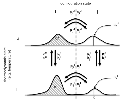
Figure 1: Illustration of the expanded transition process in xTRAM and the symbols used: $c_{ij}^{I}$ and $p_{ij}^{I}$ are transition counts and probabilities between different configuration states $i$, $j$ at the same thermodynamic state $I$. $b_{i}^{IJ}$ and $p_{i}^{IJ}$ are transition counts and probabilities between different thermodynamic states $I$, $J$ at the same configuration state $i$. The latter are constructed such that reweighting to the equilibrium densities $\mu_{\mathbf{x}}^{I}$, $\mu_{\mathbf{x}}^{J}$ of configurations $\mathbf{x}$ at different thermodynamic states $I$, $J$, occurs.

The expanded transition matrix $\mathbf{\tilde{P}}$ is defined as the maximum likelihood reversible transition matrix given $\mathbf{\tilde{N}}$. The key step in xTRAM is to estimate $\mathbf{\tilde{P}}$ from $\mathbf{\tilde{N}}$ so as to compute the expanded stationary distribution $\widetilde{\boldsymbol{\pi}}^{\top}=\widetilde{\boldsymbol{\pi}}^{\top}\mathbf{\tilde{P}}$, which has the structure

$$\widetilde{\boldsymbol{\pi}}^{\top} =(w^{1}\boldsymbol{\pi}^{1},...,w^{m}\boldsymbol{\pi}^{m}),$$ (13)

consisting of subvectors, $\boldsymbol{\pi}^{I}=(\pi_{1}^{I},...,\pi_{n}^{I})$, each containing the normalized equilibrium probabilities of configuration states $i$ given that the system is at thermodynamic state $I$. The weights $w^{I}$, normalized to $\sum_{I}w^{I}=1$, scale all subvectors such that the expanded equilibrium vector is also normalized, $\sum_{i}\sum_{I}w^{I}\pi_{i}^{I}=1$.

Data preparation and configuration-state transition counts

We process all trajectory data as follows. Each sample $\mathbf{x}$ occurring in a trajectory at time $t$ is selected when a successor sample $\mathbf{y}$ at time $t+\tau$ exists such that the trajectory fragment $\mathbf{x}\rightarrow\mathbf{y}$ was generated using the same dynamics (i.e. without intermediate changes of the thermodynamic state).

All such samples $\mathbf{x}$ are sorted into sets $S_{i}^{I}$ according to their configuration state $i$ and thermodynamic state $I$. The configuration-state transition counts

$$c_{ij}^{I}=\left|\{(\mathbf{x}\in S_{i}^{I},\mathbf{y}\in S_{j})\}\right|$$

count the number of transitions from all samples $\mathbf{x}$ in $S_{i}^{I}$ to target configuration state $j$ ($\mathbf{y}$ itself can be at any thermodynamic state as long as the dynamics to reach $\mathbf{y}$ from $\mathbf{x}$ was realized at thermodynamic state $I$). These counts yield $m$ count matrices $\mathbf{C}^{1},...,\mathbf{C}^{m}$.

We define the total counts $N$, total counts at thermodynamic state $I$, $N^{I}$, and total counts at thermodynamic state $I$ and configuration state $i$:

$$N_{i}^{I} :=\sum_{j}c_{ij}^{I}$$ (14)

$$N^{I} :=\sum_{i}N_{i}^{I}$$ (15)

$$N :=\sum_{I}N^{I}.$$ (16)

Note that the xTRAM estimations will not depend on the choice of $\tau$ provided that the count matrices $\mathbf{C}^{I}$ are obtained from simulations that ensure a local equilibrium within each starting state $S_{i}^{I}$. If this is the case, $\tau$ can be chosen arbitrarily short, e.g. equal to the interval at which the sampled configuration are saved. In practice, deviations from local equilibrium can be significant for certain simulation setups and for poor choices of the discretization, but can be compensated by using longer lag times (see random swapping results, below). When local equilibrium is not ensured by the simulation setup, TRAM estimates should be performed for a series of $\tau$-values, and then choosing the smallest $\tau$-value for which converged estimates are obtained.

Thermodynamic-state transition counts

The elements $I,J$ of the thermodynamic-state count matrix at configuration state $i$ are constructed by attributing to each sample $\mathbf{x}$ at thermodynamic state $I$ a single count that is split to all target thermodynamic states $J$ proportional to the respective probability $p^{IJ}(\mathbf{x})$:

$$b_{i}^{IJ}=\sum_{\mathbf{x}\in S_{i}^{I}}p^{IJ}(\mathbf{x}),$$ (17)

where $p^{IJ}(\mathbf{x})$ is the transition probability to thermodynamic state $J$ given that the system is at configuration $\mathbf{x}$ and thermodynamic state $I$. In the example of a multi-temperature simulation, $p^{IJ}(\mathbf{x})$ can be interpreted as the probability for which a hypothetical simulated tempering trial from temperature $I$ to $J$ would be accepted at configuration $\mathbf{x}$. In a more general setting, the transition probabilities between thermodynamic states can be derived from Bennett’s acceptance ratio Bennett (1976). From $\sum_{J}p^{IJ}(\mathbf{x})=1$, it directly follows that $N_{i}^{I}=\sum_{J}b_{i}^{IJ}$. Different choices for $p^{IJ}(\mathbf{x})$ are possible as long as they respect detailed balance.

The statistical weights $w^{I}$ of thermodynamic states in the expanded ensemble are chosen as the fraction of samples seen at each thermodynamic state $I$:

$$w^{I} :=\frac{N^{I}}{N}.$$ (18)

It will be shown later that this choice leads to a statistically optimal estimator. As an example, consider a replica-exchange simulation, all replicas $I$ are propagated in parallel and therefore $N^{1}=...=N^{m}$, resulting in equal weights $w_{I}=1/m$. When the input data stems from simulated tempering simulations between different temperatures $I$, the fraction of time spent at each temperature depends on the choice of the simulated tempering weights Marinari and Parisi (1992), and could therefore be different. With choices given by Eq. (18), the absolute probability of configuration $\mathbf{x}$ in the expanded ensemble is:

$$\mu^{I}(\mathbf{x})=w^{I}\rho^{I}(\mathbf{x})=\frac{N^{I}}{N}e^{f^{I}-u^{I}(\mathbf{x})}.$$ (19)

In order for the thermodynamic-state transition process to sample from the correct statistical weights, it must fulfill the detailed balance equations:

$$\mu^{I}(\mathbf{x})\,p^{IJ}(\mathbf{x})=\mu^{J}(\mathbf{x})\,p^{JI}(\mathbf{x}).$$ (20)

Various choices for $p^{IJ}(\mathbf{x})$ can be made that meet these constraints. It will turn out that the statistically optimal choice is to a thermodynamic state $J$ according to its equilibrium probability of that state in the expanded ensemble, i.e.:

$$p^{IJ}(\mathbf{x})=\frac{\mu^{J}(\mathbf{x})}{\sum_{K}\mu^{K}(\mathbf{x})}=\frac{N^{J}e^{f^{J}-u^{J}(\mathbf{x})}}{\sum_{K}N^{K}e^{f^{K}-u^{K}(\mathbf{x})}}.$$ (21)

The choices (19) and (21) obviously fulfill the detailed balance equations (20). Using Eq. (21) in an implementation requires shifting the absolute energy value in order to avoid numerical overflows when evaluating the exponential (see Appendix of Shirts and Chodera (2008) for a discussion).

An alternative choice for the thermodynamic-state transition process is the Metropolis rule, which is easier to implement and produced indistinguishable results compared to choice (21) in our applications:

$$p^{IJ}(\mathbf{x}) =\frac{N^{I}}{N}\min\left\{1,\frac{N^{J}\mathrm{e}^{f^{J}-u^{J}(\mathbf{x})}}{N^{I}\mathrm{e}^{f^{I}-u^{I}(\mathbf{x})}}\right\}\>\>\>\>\>\>I\neq J$$ (22)

$$p^{II}(\mathbf{x}) =1-\sum_{J\neq I}p^{IJ}(\mathbf{x}).$$

Free energies:

In order to compute $p^{IJ}(\mathbf{x})$ in Eq. (17) using Eq. (21) or (22), an estimate of the free energies $f^{I}$ is needed. At initialization, the $f^{I}$’s are estimated using Bennett’s acceptance ratio Bennett (1976). To this end, the thermodynamic states simulated at, are sorted in a sequence $(1,\>...,I,\>I+1,\>...,\>m)$, e.g. ascending temperatures. The free energies are then initially set to:

$$f^{1} :=0$$ (23)

$$f^{I+1} :=f^{I}-\ln\frac{\frac{1}{N^{I}}\sum_{\mathbf{x}\in S^{I}}\min\{1,\mathrm{e}^{u^{I}(\mathbf{x})-u^{I+1}(\mathbf{x})}\}}{\frac{1}{N^{I+1}}\sum_{\mathbf{x}\in S^{I+1}}\min\{1,\mathrm{e}^{u^{I+1}(\mathbf{x})-u^{I}(\mathbf{x})}\}},$$ (24)

where the sample averages are taken over all samples in a given thermodynamic state, as denoted by $\mathbf{x}\in S^{I}$. In subsequent iterations, we can update the free energies using:

$$f^{I,\,\mathrm{new}}:=f^{I}-\ln\frac{N}{N^{I}}\sum_{i}\tilde{\pi}_{i}^{I}.$$ (25)

The iteration is converged when in the expanded equilibrium distribution $\boldsymbol{\tilde{\pi}}$ has weights equal according to the target values $w^{I}$: $\sum_{i}\tilde{\pi}_{i}^{I}=\frac{N^{I}}{N}$ for all $I$. Eq. (25) will adapt $f^{I}$ until this equilibrium is achieved (see supplementary information for details).

Estimation of the equilibrium distribution

In every iteration, we obtain a transition count matrix possessing the sparsity structures sketched in (12). Because the theory is based on a transition matrix fulfilling detailed balance, we can estimate $\mathbf{\tilde{P}}$ using the reversible transition matrix estimator described in Prinz et al. (2011) which also provides the expanded equilibrium distribution $\boldsymbol{\tilde{\pi}}$ as a by-product.

However, we can derive a simple direct estimator for $\boldsymbol{\tilde{\pi}}$ without going through $\mathbf{\tilde{P}}$ (see supplementary information I.D). Let $x_{i}^{I}$ be variables that are iterated to approximate $\pi_{i}^{I}$. Then iterating the update:

$$x_{i}^{I,\>\mathrm{new}} =\frac{1}{2}\sum_{j=1}^{n}\frac{c_{ij}^{I}+c_{ji}^{I}}{\frac{N_{i}^{I}}{w^{I}\pi_{i}^{I}}+\frac{N_{j}^{I}}{w^{I}\pi_{j}^{I}}}+\frac{1}{2}\sum_{J=1}^{m}\frac{b_{i}^{IJ}+b_{i}^{JI}}{\frac{N_{i}^{I}}{w^{I}\pi_{i}^{I}}+\frac{N_{i}^{J}}{w^{J}\pi_{i}^{J}}}$$ (26)

$$\pi_{i}^{I,\>\mathrm{new}} =\frac{x_{i}^{I}}{\sum_{j=1}^{n}x_{j}^{I}}.$$ (27)

converges towards the maximum likelihood estimate of $\pi_{i}^{I}$. The xTRAM estimator is summarized in algorithm 1.

1. Compute the largest connected set from the projection of the multi-temperature trajectory ensembles onto states. All vectors and matrices are defined on that connected set. For all other states, $\pi_{i}^{I}$ is set to 0.

2. Initial guess of free energies: set $f_{1}:=0$ and for $I=1,...,m-1$ set:

   $$f^{I+1}:=f^{I}-\ln\frac{\frac{1}{N^{I}}\sum_{\mathbf{x}\in(*,I)}\min\{1,\mathrm{e}^{u^{I}(\mathbf{x})-u^{I+1}(\mathbf{x})}\}}{\frac{1}{N^{I+1}}\sum_{\mathbf{x}\in(*,I+1)}\min\{1,\mathrm{e}^{u^{I+1}(\mathbf{x})-u^{I}(\mathbf{x})}\}}.$$

3. Compute configuration-state counts $\mathbf{C}^{I}=(c_{ij}^{I})$. $c_{ij}^{I}$ is the number of times a trajectory simulated at thermodynamic state $I$ was found to be at configuration state $i$ at time $t$, and at state $j$ at time $t+\tau$.
   Define $N_{i}^{I}:=\sum_{j}c_{ij}^{I}$, $N^{I}:=\sum_{i}N_{i}^{I}$, $N:=\sum_{I}N^{I}$.

4. Initial guess of equilibrium probabilities:

   $$\pi_{i}^{I}:=\frac{N_{i}^{I}}{N^{I}}.$$

5. Iterate to convergence of $f^{I}$:

   1. Compute thermodynamic-state counts by

      $$b_{i}^{IJ}:=\sum_{x\in S_{i}^{I}}p^{IJ}(\mathbf{x}),$$

      with $p^{IJ}(\mathbf{x})$ from Eq. (21) or (22).

   2. Iterate to convergence of $\pi_{i}^{I}$ using $w^{I}:=N^{I}/N$:

      $$x_{i}^{I,\,\mathrm{new}} :=\sum_{j}\frac{c_{ij}^{I}+c_{ji}^{I}}{\frac{N_{i}^{I}}{w^{I}\pi_{i}^{I}}+\frac{N_{j}^{I}}{w^{I}\pi_{j}^{I}}}+\sum_{J}\frac{b_{i}^{IJ}+b_{i}^{JI}}{\frac{N_{i}^{I}}{w^{I}\pi_{i}^{I}}+\frac{N_{i}^{J}}{w^{J}\pi_{i}^{J}}}$$

      $$\pi_{i}^{I\,\mathrm{new}} :=\frac{x_{i}^{I}}{\sum_{I}\sum_{j}x_{j}^{I}}.$$

   3. Update free energies:

      $$f^{I}:=f^{I}-\ln\frac{N}{N^{I}}\sum_{i}\pi_{i}^{I}.$$

Algorithm 1 xTRAM Algorithm for estimating the free energies $f^{I}$ and equilibrium probabilities $\pi_{i}^{I}$.

Estimation of arbitrary expectation functions

Now we can derive an efficient estimator of the equilibrium expectation values $\langle A\rangle$ of an arbitrary function $A(\mathbf{x})$, as defined by Eq. (10), at an arbitrary thermodynamic state (possibly not simulated at). For this we employ Eqs. (14-15) in Shirts and Chodera (2008), treating every configuration state at every thermodynamic state as a separate MBAR thermodynamic state. We define the weights:

$$g(\mathbf{x})=\frac{\mathrm{e}^{-u(\mathbf{x})}}{\sum_{K}\sum_{i}N_{i}^{K}\mathrm{e}^{f_{i}^{K}-u^{K}(\mathbf{x})}},$$ (28)

where the configuration free energies can be computed as $f_{i}^{I}=f^{I}-\ln\pi_{i}^{I}$. As shown in the supplementary information, the expectation values of an arbitrary function of configuration, $\langle A\rangle$ can thus be estimated as

$$\langle A\rangle=\frac{\sum_{\mathbf{x}}g(\mathbf{x})\,A(\mathbf{x})}{\sum_{\mathbf{x}}g(\mathbf{x})},$$ (29)

where $\sum_{\mathbf{x}}$ runs over all samples in the data.

II.4 Asymptotic correctness of the xTRAM estimator

The exact transition probability between sets $S_{i}$ and $S_{j}$ at thermodynamic state $I$ is given by:

$$p_{ij}^{I} =\frac{1}{\pi_{i}^{I}}\int_{S_{i}}d\mathbf{x}\>\mu^{I}(\mathbf{x})\int_{S_{j}}d\mathbf{y}\>p^{I}(\mathbf{x},\mathbf{y};\,\tau),$$ (30)

where $p^{I}(\mathbf{x},\mathbf{y};\,\tau)$ is the probability density of the system to be in configuration $\mathbf{y}$ at time $t+\tau$ given that it is in configuration $\mathbf{x}$ at thermodynamic state $I$ at time $t$. By definition, microscopic detailed balance holds for the dynamics at thermodynamic state $I$: $\mu^{I}(\mathbf{x})\,p^{I}(\mathbf{x},\mathbf{y};\,\tau)=\mu^{I}(\mathbf{y})\,p^{I}(\mathbf{y},\mathbf{x};\,\tau)$. Using detailed balance in (30) directly leads to:

$$\pi_{i}^{I}p_{ij}^{I}=\pi_{j}^{I}p_{ji}^{I}.$$ (31)

The exact thermodynamic state transition probability from thermodynamic state $I$ to $J$ at configuration state $i$ is given by:

$$p_{i}^{IJ}=\frac{1}{w^{I}\pi_{i}^{I}}\int_{S_{i}}d\mathbf{x}\>\mu_{\mathbf{x}}^{I}p_{\mathbf{x}}^{IJ}.$$ (32)

Together with (20), we have detailed balance in discrete states:

$$w^{I}\pi_{i}^{I}p_{i}^{IJ}=w^{J}\pi_{i}^{J}p_{i}^{JI}.$$ (33)

In the statistical limit $N\rightarrow\infty$, which can be either realized by trajectories of great length, or by a large number of short trajectories, our expected transition counts converge to the following limits:

$$\hat{c}_{ij}^{I} =\lim_{N\rightarrow\infty}c_{ij}^{I}=N_{i}^{I}p_{ij}^{I}$$ (34)

$$\hat{b}_{ij}^{I} =\lim_{N\rightarrow\infty}b_{ij}^{I}=N_{i}^{I}p_{i}^{IJ}.$$ (35)

Plugging these counts and the reversibility conditions (31,33) into the estimator of equilibrium probabilities (98), we obtain the accurate result:

$$x_{i}^{I}=w^{I}\pi_{i}^{I}.$$ (36)

Furthermore, in the statistical limit, the Bennett acceptance ratio initialization (Algorithm 1, step 2.) is exact. With result (36), this estimate is not changed in Algorithm 1, step 5c. Thus, the xTRAM estimator converges to unbiased estimates of all equilibrium properties (7-10) in the statistical limit.

II.5 Special cases

With one thermodynamic state, xTRAM is a Markov model

Consider the situation that simulations were conducted at a single thermodynamic state, such as unbiased molecular dynamics simulations of a macromolecule at a fixed temperature $I$. The xTRAM count matrix is now an $n\times n$ configuration state count matrix $\mathbf{C}=(c_{ij})$.

We only have one free energy $f^{1}=0$. Using Eq. (9), the configuration free energies are given by $f_{i}^{I}=-\ln\pi_{i}$, where $\pi_{i}$ are the estimated equilibrium probabilities of discrete configuration states $i$. These equilibrium probabilities can be obtained by the special case of Eq. (98,99):

$$x_{i}^{\mathrm{new}} =\sum_{j=1}^{n}\frac{c_{ij}+c_{ji}}{\frac{N_{i}}{\pi_{i}}+\frac{N_{j}}{\pi_{j}}}$$ (37)

$$\pi_{i}^{\mathrm{new}} =\frac{x_{i}}{\sum_{j=1}^{n}x_{j}}.$$ (38)

Eqs. (37-38) is the equilibrium probability of the maximum likelihood $n\times n$ reversible transition matrix given count matrix $\mathbf{C}$. Therefore, in the single-thermodynamic state case our estimates are identical to those of a reversible Markov model.

Standard methods can be used to compute the maximum likelihood reversible transition matrix $\mathbf{P}$ Prinz et al. (2011); Bowman et al. (2009). However, if we wish to use $\mathbf{P}$ to extract not only stationary but kinetic information, the lag time $\tau$ used to obtain the count matrix $\mathbf{C}$ must be chosen sufficiently large in order to obtain an accurate estimate Prinz et al. (2011).

When all thermodynamic states are in global equilibrium, xTRAM is identical to MBAR in the estimation of $f^{I}$

In order to show the relationship between TRAM and MBAR, we use the TRAM equations (25,98-99), and specialize them using the MBAR assumption that each thermodynamic state is sampled from global equilibrium. This assumption can be modeled by merging all configuration states to one state. When converged, the TRAM quantities then fulfill the equations:

$$\pi^{I}p^{IJ} =\frac{b^{IJ}+b^{JI}}{\frac{N^{I}}{\pi^{I}}+\frac{N^{J}}{\pi^{J}}}$$ (39)

$$0 =-\ln\frac{N}{N^{I}}\pi^{I}.$$ (40)

By combining these equations with (17) and (21) (see Supplementary Information for details), we obtain:

$$f^{I}=-\ln\sum_{\mathrm{all}\>\mathbf{x}}\frac{e^{-u^{I}(\mathbf{x})}}{\sum_{K}N^{K}e^{f^{K}-u^{K}(\mathbf{x})}},$$ (41)

which is identical to the MBAR estimator for the reduced free energy of thermodynamic state $I$ (See Eq. (11) in Shirts and Chodera (2008).

The MBAR and xTRAM estimators of $\pi_{i}^{I}$ are consistent

Using again the condition that all simulations are in their respective global equilibria, and tending to the statistical limit $N\rightarrow\infty$ (see Supplementary Information for details), we can show that the xTRAM estimate for the equilibrium probabilities $\pi_{i}^{I}$ can be written as:

$$\pi_{i}^{I}=\frac{\sum_{\mathbf{x}\in S_{i}}\frac{e^{-u^{I}(\mathbf{x})}}{\sum_{K}N^{K}e^{f^{K}-u^{K}(\mathbf{x})}}}{\sum_{\mathrm{all}\>\mathbf{x}}\frac{e^{-u^{I}(\mathbf{x})}}{\sum_{K}N^{K}e^{f^{K}-u^{K}(\mathbf{x})}}},$$ (42)

which is identical to the MBAR expectation value for $\pi_{i}^{I}$ (to obtain this result, use Eqs. (14-15) in Shirts and Chodera (2008) with the indicator function on set $S_{i}$).

II.6 Random swapping (RS) simulations

PT, ST and REMD simulation protocols are constructed such that they sample from global equilibrium at all temperatures after a sufficiently long burn-in phase. Global equilibrium is ensured by constructing appropriate Metropolis acceptance criteria for temperature swaps. The disadvantage is that to ensure a good mixing rate between replicas, dense replica spacing is required - a problem that becomes increasingly difficult for systems with a large number of degrees of freedom, as is the case of biomolecular simulations of $10^{5}$ or more atoms.

However, due to the use of transition matrices, xTRAM only requires local equilibrium within the discrete configurational states rather than global equilibrium - a much weaker requirement. It is thus tempting to consider using a simulation protocol that is much more efficient than PT, ST and REMD while sacrificing the property that it samples from global equilibrium at all temperatures. Such a protocol would be useful if it is still possible to recover the correct stationary probabilities using xTRAM. One can consider the simple random swapping (RS) protocol, in which the replica makes a random walk in a pre-defined set of temperatures $T^{1},...,T^{m}$. Every so many MD/MC simulation steps, the replica jumps up or down in temperature with equal probability. The temperature move is always accepted unlike in ST. In this way temperature and configuration space can be efficiently sampled with very widely spaced replicas providing a good set of input trajectories for xTRAM.

Because there is no Metropolis-Hastings acceptance criterion involved, the initial samples after each temperature swap are definitely out of global, but also out of local equilibrium at the new temperature. While discarding an initial fragment of the data would seem to be a viable option, it turns out that instead using larger lag times $\tau$ appears to work much better in correcting the estimates, as established for Markov model construction Prinz et al. (2011). However, a solid theory for this observation has yet to be found, which is beyond the scope of the current paper.

III Results

To demonstrate the validity and resulting advantage of the proposed estimator, two Langevin processes in model potentials, and two explicitly solvated molecular dynamics processes are considered. In all cases we will compare three different estimators, which are the newly proposed xTRAM estimator, MBAR and histogram counting (direct counting estimate), each applied to the same sets of data. Both accuracy and precision of all methods will be looked at by evaluating the systematic and statistical error for representative discrete states and temperatures of interest.

III.1 Two-well potential with solvent degrees of freedom

As a first example we consider Langevin dynamics in an asymmetric double well potential (Fig. 2(A)) with corresponding stationary (Boltzmann) distribution $P(x)$ shown in Fig. 2(B) for the reduced temperature $k_{B}T=1$. In order to make the system more complex, we add a set of $N$ solvent particles. Each solvent coordinate $i$ is subject to a harmonic potential $U(y_{i})=y_{i}^{2}$, where $y_{i}$ is the particle’s position.

The state space is discretized into two states, corresponding to the two potential basins. We aim to estimate the equilibrium distribution of these two states, from a set of different multi-temperature simulation protocols in combination with any of the estimators considered (xTRAM, MBAR and direct counting). All simulations are initiated from a local stationary distribution in state $S_{1}$ and the three different simulation protocols chosen are parallel tempering (PT), simulated tempering (ST) and random swapping (RS) simulations. With each simulation protocol 100 independent realizations were generated and their results are shown in Fig. 2. For all three simulation protocols a temperature space needs to be defined, consisting of four exponentially spaced temperatures between $k_{B}T$=1 and $k_{B}T=10$ in reduced units, for fig. 2(C)-(F) and six exponentially spaced temperatures between $k_{B}T=1$ and $k_{B}T=15$ in reduced units for fig. 2(G)-(H). The temperatures are chosen in such a way that barrier crossings at the lowest temperature are very rare events. For more details on the simulation protocols and setup see the supplementary information.

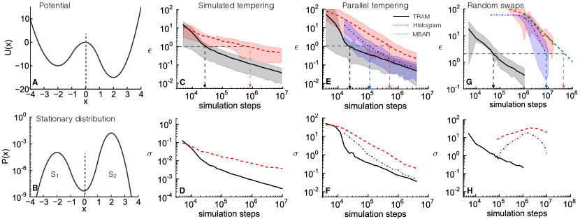
Figure 2: (A) Double-well potential $U(x)$. (B) Corresponding stationary distribution at a reduced temperature $k_{B}T=1$. (C+D) Results of the ST simulation. (C) The relative error of $\pi_{1}$ is shown w.r.t the number of simulation steps for simulations with two solvent particles and four temperatures. The direct histogram estimate (red, dashed) and xTRAM (black, continuous line) are evaluated on the same data set. (D) Standard deviation ($\sigma$) from 100 realizations are shown w.r.t. simulation steps taken for direct count histogram (red, dashed) and xTRAM (black, continuous). (E+F) Results of the PT simulation. (E) relative error $\pi_{1}$ w.r.t. to simulation steps from PT simulations over 100 realizations for direct counts (red, dashed), MBAR (blue, dashed dotted) and xTRAM (black continuous) (F) Standard deviation from data in (E). (G+H) Results of a system with $N=50$ solvent particles using PT simulations for the MBAR and direct counting estimate and RS simulations for the xTRAM estimate. (G) relative error w.r.t. total number of simulation steps for 20 temperature replica PT simulations direct count histograms (red, dashed) MBAR (blue, dashed dotted) comparing to xTRAM (black, continuous) analysis of RS simulation with six temperatures. The dashed green line shows a fit of $t^{-0.5}$ to the tail of the relative error. (H) shows standard deviations of data in (G).

Fig. 2(C-D) and (E-F) show the results of ST and PT simulations with two solvent particles respectively. The results are displayed in form of a log-log plot of the relative error of the estimate of $\pi_{1}$ and its convergence behavior with increased simulation time. The relative error is given by:

$$\epsilon=\Big{|}\frac{\pi(S_{1})_{\mathrm{exact}}-\pi(S_{1})_{\mathrm{estimate}}}{\pi(S_{1})_{\mathrm{exact}}}\Big{|}.$$ (43)

The stationary distribution, at the lowest reduced temperature of $k_{B}T=1$ is obtained using all three estimators: (1) direct counting, (2) MBAR and (3) xTRAM. Fig. 2(C), (E) and (G) report averages and confidence intervals of the time-dependent relative errors computed from $100$ realizations of each simulation. Fig. 2(D), (F) and (H) report standard deviations ($\sigma$) of the simulation data from 100 independent realizations and their time dependence. In panels (C) and (E) the tail of the mean error for all three methods decays approximately equal to $b/\sqrt{t}$, where $b$ is a constant related to the decorrelation time $t_{\mathrm{corr}}$ required to generate an uncorrelated configuration at the temperature analyzed. Arrows in panel (C) and (E) indicate a relative error of 1. In the case of the ST simulation xTRAM outperforms direct counting by a factor of 40 and in (E) for the parallel tempering simulation xTRAM has a gain of a factor of five over MBAR estimates and a factor of 25 over direct counting estimates. This means that the xTRAM estimates converge up to a 40 fold faster in comparison to direct counts and at least five fold faster in comparison to MBAR, indicating that the decorrelation time with xTRAM can be much shorter. Consequently, less simulation time needs to be invested when the data is analyzed with xTRAM. Secondly the, standard deviation as seen in (D) and (F) is consistently lower for xTRAM, meaning that over independent realizations, the accuracy of the estimate is better in comparison to MBAR and direct counting.

Additional efficiency can be gained when the simple random swapping (RS) simulation protocol can be employed instead of ST or PT simulations, because then the number of replicas can be reduced such that TRAM gives good results, while ST or PT replicas would not mix well in temperature space. In Fig. 2(G) the results of a simulation with $50$ solvent particles are depicted. In order to achieve a good mixing in a PT simulation, 20 temperatures exponentially spaced in the range of 1 to 15 in reduced units need to be used, which is compared to a 6 replica RS simulation (see supplementary information for more details). The lag time $\tau$ for the evaluation could actually be chosen as small as the saving interval of the simulation in this case, resulting in the same convergence as using larger lag times. Looking at a relative error of $\epsilon=2$, an extrapolation needs to be made to compute how many simulation steps are needed for the PT direct counting estimate. From the extrapolated convergence behavior it is found to be around $1\times 10^{8}$ simulation steps. Despite the fact that the RS protocol itself is not in equilibrium, the correct equilibrium probabilities can be recovered when used in conjunction with xTRAM. In this case, a relative error $\epsilon=2$ is achieved at around $1\times 10^{5}$ simulation steps, indicating an efficiency gain of around three orders of magnitude for RS/TRAM and more than two orders of magnitude over MBAR used with the same PT simulation data as for the direct counts. It should be stressed again, that for MBAR and direct counting only simulations sampling from a global equilibrium can be used, therefore these estimators are not suitable to be used in conjunction with a random swapping simulation. Fig. 2(H) shows the standard deviation of the relative error from 100 realizations. Initially, the standard deviation is deceptively small for direct counts and MBAR, because many of the 100 simulations have only seen state 1. The standard deviation increases, as the second state is discovered reaching a peak, from which onwards $\sigma$ decreases again.

III.2 Simple protein folding model

In order to illustrate the limitations of the method, we now discuss an example where xTRAM offers no significant advantage over the established MBAR estimator. We consider an idealized folding potential with an energetically stabilized native state and an entropically stabilized denatured state. The state space is spanned by a vector in $5$ dimensions, such that $\mathbf{{x}\in}\mathbb{R}^{5}$ and $r=|\mathbf{x}|$ is the distance from zero. The potential is defined as:

$$U(r)=\begin{cases}-2.5(r-3)^{2}&\mathrm{if}\;r<3\\ 0.5(r-3)^{3}-(r-3)^{2}&\mathrm{if}\;r\geq 3\end{cases}$$ (44)

and depicted in Fig. 3(A). Again a Langevin dynamics simulation was carried out with more details provided in the supplementary information. The system is discretized into two states: native and denatured, with a state boundary at $r=2.7$, representing the distance around which the lowest probability density is observed. All simulations are initiated in the native state.

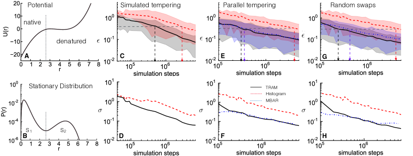
Figure 3: (A) Potential $U(r)$. (B) Corresponding stationary distribution at $\frac{1}{\beta}=1.1k_{B}T$. Results are shown in terms of the relative error $\epsilon$ of the probability of being in the “denatured” state versus the number of simulation steps required. (C)-(D) Results of the ST simulation. (C) black continuous line xTRAM estimate, red dashed line direct counting estimate. Arrows indicate an $\epsilon=0.3$ error level (D) standard deviation of the 100 realizations from (C) for both estimators. (E)-(F) Results of the parallel tempering simulation. (E) In blue dashed dotted the MBAR estimate, arrows indicate $\epsilon=0.2$ error level. (F) standard deviation of data in (E) from 100 realizations. (G)-(H) Comparison of RS + xTRAM estimate to the PT estimate using MBAR and direct counts in (E). Arrows indicate $\epsilon=0.2$ error level. (H) standard deviation of the data in (G) over 100 realizations.

The potential and the exact stationary density $\pi(r)$ at $\frac{1}{\beta}=1.1k_{B}T$ are shown in Fig. 3(A) and (B) respectively. Note that the denatured state is stabilized by entropy, as more microstates are available for $r>2.7$ than for $r<2.7$. The convergence of the estimate of the relative error, Eq. (43) of the unfolded state is measured for a set of ST, PT and RS simulations. Results are taken from $100$ different realizations and six exponentially spaced temperatures between $\frac{1}{\beta}=1.1k_{B}T$ and $\frac{1}{\beta}=1.7k_{B}T$. Panel (C) and (D) of Fig. 3 show the results of the ST simulation, comparing the convergence of direct counting against xTRAM of the relative error of being in the denatured state. As before, xTRAM is shown by the black, continuous line, direct counting by the dashed, red line. Arrows indicating an error level of $\epsilon=0.3$ are used as guidance for the comparison of the convergence. Using xTRAM as the estimator for the analysis of the simulation results in a nine fold gain over direct counting. Shaded areas indicate confidence intervals. Fig. 3(D) shows the convergence of the standard deviation obtained from 100 independent realizations of the ST simulation from (C). The standard deviation of the xTRAM estimate is consistently lower than for the direct counting estimate. Fig. 3(E) and (F) summarize the results of the parallel tempering simulations. Here an 11 fold gain is observed when using xTRAM over direct counting, but MBAR and xTRAM perform almost equally as well, indicated by the arrows shown at an error level of $\epsilon=0.2$. This behavior suggests, that in this model samples from the local and global equilibrium are generated at the same rate. Fig. 3 (F) shows the standard deviation of the data in (E) from the 100 independently generated simulations.

Fig. 3(G) and (H), compare the direct counting and MBAR estimate of (E) with an RS simulation using only a single replica and 4 exponentially spaced temperatures between $k_{B}T=[1.1\ldots 1.7]$. Now xTRAM has a 2 fold gain over MBAR.

As xTRAM is a local-equilibrium generalization of MBAR, it is guaranteed to have equal or better estimation accuracy. However, the results above indicate that the accuracy gain of xTRAM over MBAR can be small in some systems. In the folding potential this is presumably due to the fact that the different temperatures not only help in barrier crossing, but give rise to vastly different equilibrium probabilities of the folded state (stable at low temperatures) and the unfolded state (stable at high temperatures). Thus, even at short simulation times, both the folded and unfolded states are present in the replica ensemble and can successfully be reweighted using MBAR without relying on too many actual configuration state transitions. xTRAM will gain efficiency in situations, where the state space exploration is slowed down by higher friction or additional barriers, as often found in macromolecules.

III.3 Alanine dipeptide

In order to test the xTRAM estimator on a system with many degrees of freedom, we turn to molecular dynamics (MD) simulations using an explicit solvent model. To this end we study solvated alanine dipeptide, a small and well-studied peptide with multiple metastable states Chekmarev et al. (2004); Smith (1999); Chodera et al. (2006); Du et al. (2011) and around $6000$ degrees of freedom in the case of the system set-up used here. Alanine dipeptide was prepared using an explicit water model and simulated in the MD software package OpenMM Eastman et al. (2013). All the necessary simulation details are provided in the appendix.

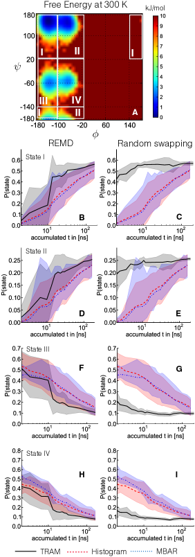
Figure 4: (A) Free energy with a 10 $\mathrm{kJ/,mol}$ cutoff, indicating discrete states. (B, D, F, H) REMD simulation convergence of state probability over ten realizations. Estimates are obtained from xTRAM (black, continuous line), MBAR (blue, dashed-dotted line), and direct counting (red, dashed line). (C, E, G, I) RS simulation convergence of state probabilities over five realizations, compared to REMD simulation estimates using MBAR and direct counts.

The dominant conformations of this system are the different rotamers set by the dihedral angles $\psi$ and $\phi$. This means we are interested in estimating the free energy surface in $\phi$/$\psi$ space at a low temperature of interest. Again, we are interested in extracting the stationary probabilities of metastable basins at different temperatures. However, the system at $T=300\,K$ is not very metastable, thus we introduce an artificial metastability to the torsional angles. For this purpose we add a potential to the minima of the $\phi$ and $\psi$ dihedral angles in order to extend the time the system stays in a particular angular configuration. The ideal choice of such an additional potential are periodic von Mises potentials of the form:

$$U(\delta)=\epsilon\exp\Big{(}\frac{\kappa\cos(\delta-\delta_{0})}{2\pi I_{0}}\Big{)},$$ (45)

where $I_{0}$ is a zeroth order Bessel function and $\delta$ is the angle to which the additional potential is added. For more details see the supplementary information. We use two different types of multi-temperature simulations: a set 10 independent realizations of a 32 temperature REMD simulation with temperatures exponentially spaced in the range of $T=[300K\,-600K]$ and a set of independent independent realizations of a 13 temperature RS simulation, where only every third temperature out of the REMD multi-temperature ensemble was used. From the 10 REMD trajectories the last 1 ns of each were used to estimate the free energy surface in dihedral $\phi$ and $\psi$ space as shown in Fig. 4(A). From the free energy surface four discrete states could be defined, numbered, and highlighted by the white boxes. All simulations were initiated in state IV. From the simulations dihedral coordinates, discrete trajectories were generated which then allow a stationary estimate through direct counts of the frequency of each state visited along the trajectory (in the case of the REMD simulation). The same discrete trajectories are also used for xTRAM and MBAR estimation.

For the RS simulation the total simulation time was less, as only 13 instead of the 32 parallel replicas were simulated. Confidence intervals are indicated by the shaded regions calculated over the independent realizations of every simulation type. In order for the RS simulation to produce valid results the lag-time at which the data points are used needs to be adjusted, the saving interval of the trajectory was 0.1 ps and and the lag interval at which data frames were used was chosen to be $\tau=$1 ps and temperature switches were carried out every 10 ps, for more details on the RS simulation refer to the supplementary information.

Fig. 4(B), (D), (F), and (H) show the convergence results of the REMD simulation. While all estimators yield similar (and inaccurate) estimates for very short simulation times, xTRAM exhibits considerable advantages over MBAR and direct counting after 10 ns simulation time. The fastest-converging estimator (see below) produces stable equilbrium probabilities of about $(0.57,0.25,0.13,0.1)$ for states 1-4 at 100 ns simulation time. Using REMD data, xTRAM converges to within about 10% of these values with roughly one order of magnitue simulation data compared to MBAR and direct counting (20 ns versus 200 ns).

Fig. 4(C), (E), (G), and (I) compare the performance of the RS simulations when analyzed with xTRAM, in comparison to the standard REMD simulations. As a result of the smaller number of replicas required and the enhanced mixing properties, another order of magnitude is gained with the RS protocol when comparing to the xTRAM estimate of the REMD simulations. Since xTRAM is currently the only available estimator to unbias RS simulations, the advantage of xTRAM over MBAR and direct counting amounts two orders of magnitude (xTRAM with RS versus MBAR with REMD). This advantage of xTRAM in conjunction with RS can be much larger for systems with many degrees of freedom, where a REMD simulation would need many closely spaced replicas, thus resulting in vast computational effort and slow exchange dynamics.

III.4 Deca-alanine

Finally we consider the 10 amino acid long deca-alanine (Ala₁₀). This peptide is know to undergo a helix-coil transition, which has been studied extensively Best and Hummer (2009); Michaud-Agrawal et al. (2011); Sorin and Pande (2005); Huang et al. (2001). Ten independent runs of all-atom replica exchange simulations were conducted with the GROMACS software MD package, each using 24 exponentially spaced temperatures ranging from T = 290 K to 400 K Hess et al. (2008). We ran the simulation for 40 ns total simulation time per replica and conducted 10 independent realizations of these. For more detailed description of the simulation details see the supplementary information.

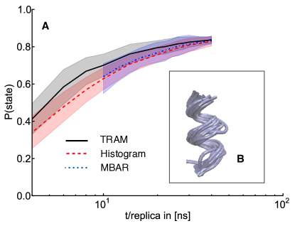
Figure 5: (A) Convergence of the probability of the system being in a helical state with respect to the total simulation time per replica. The xTRAM estimate is given by the continuous black line, the histogram count by the dashed red line, and the MBAR estimate by the dashed-dotted blue line. Confidence intervals are obtained from ten independent REMD simulations. (B) Structure averages of the helix state whose convergence is shown in (A).

In this larger molecular system the discretization of configuration space is no longer trivial. For this purpose we use time-lagged independent component analysis (TICA) on the replica trajectories of the set of C_α distances, omitting nearest neighbor distances along the peptide chain Pérez-Hernández et al. (2013). TICA is useful to identify the subspace in which the slowest transitions occur. Here, we chose three leading TICA coordinates, and used a regular spatial clustering on these with a minimum distance cutoff of 3 yielding 44 discrete clusters. This analysis was carried using the Markov model package EMMA Senne et al. (2012). See supplementary information for more details.

xTRAM, MBAR and histogram counting were used in order to estimate the equilibrium probabilities on the 44 discrete configuration states. In order to obtain a simple representation of the results, the equilibrium probabilities summed over all $\alpha$-helical states is shown in Fig. 5(B). As before, we are interested in the analysis at the lowest simulation temperature ($T$ = 290 K).

As seen in Fig 5(A) the advantage gained from TRAM in comparison to MBAR and direct counting in this case is only about two fold. However, this can be attributed to the fact, that the system does not display a very strong metastability and the slowest timescale, computed independently with a Markov state model on direct 290 K trajectories, is only 14 ns. Moreover, like the simple folding model above, Ala₁₀ has the same property that the temperatures stabilize the folded and unfolded states quite differently, leading to simultaneous observation of folded and unfolded states at early stages of the replica simulation, and also to the fact that significantly many transitions between folded and unfolded state occur only in a very small part of the replica ensemble (in the replicas around the melting point). As a result, the advantage of taking configuration-state transitions into account is smaller in this case compared to systems at which the different metastable states are present at a larger range of temperatures. As demonstrated for the simple folding model above, larger gains of computational efficiency can still be obtained by reducing the number of replicas, e.g. by employing the RS protocol in conjunction with the xTRAM estimator.

IV Discussion and Conclusion

Expanded TRAM can be used to obtain estimates of equilibrium properties from any set of simulations that was conducted at different thermodynamic states, such as multiple temperatures, Hamiltonians, or bias potentials, which we demonstrated here for multiple temperature simulations. It is therefore applicable to generalized ensemble simulations such as replica-exchange and parallel/simulated tempering, as well as umbrella sampling or metadynamics. The quantities estimated can include free energy differences, equilibrium probabilities or equilibrium expectations of functions of configuration state. As such, xTRAM has the same application scope as existing reweighting estimators (e.g. WHAM and MBAR).

In contrast to WHAM and MBAR, xTRAM does not assume simulation data to be generated from global equilibrium. Rather, xTRAM combines ideas from MBAR and Markov modeling to an estimator that makes use of both, Boltzmann reweighting of sampled configurations between thermodynamic states, and transition count statistics between different configuration states generated by contiguous trajectory segments. Compared to MBAR, estimates obtained from xTRAM can be more accurate as they suffer less from data that has not yet decorrelated from the initial configurations, as well as more precise as the statistics in the simulation data can be used more efficiently when every conditional independent transition count is useful rather than only every globally independent count.

xTRAM is an asymptotically correct estimator, i.e. its estimates converge to the exact values in the limit of long or many simulation trajectories. We have also shown that in the special case when simulation data are at global equilibrium, we can derive the MBAR equations from the expectation values of the xTRAM equations. MBAR is thus a special case of xTRAM, suggesting that the accuracy of xTRAM estimates should be at least equally good as those of MBAR estimates, but may be significantly better when parts of the simulation data are not in global equilibrium. The applications shown here confirm this result, exhibiting sometimes order-of-magnitude more accurate estimates when xTRAM is employed, and therefore allowing the use of shorter simulation times while maintaining the same accuracy in the estimate.

While MBAR provides statistically optimal (i.e. minimum-variance) estimates under the condition that data are in global equilibria, it is currently not known whether xTRAM is also statistically optimal. However, the applications in this paper suggest that the variances of xTRAM estimates are in most cases significantly better than those of MBAR or direct counting.

An interesting aspect of xTRAM is the fact that it does not rely on the data being at global equilibrium, thus opening the door to consider new simulation methods that deliberately sacrifice global equilibrium for enhanced sampling. This feature reflects the Markov-model nature of the configuration-state statistics in xTRAM - Markov models also allow to obtain unbiased estimates from short trajectories that are not sampling from global equilibrium, as long as they sample from local equilibrium within each configuration state. We have demonstrated this ability by using xTRAM to unbias simple random swapping simulations that exchange temperature replicas in complete ignorance of the Metropolis acceptance probability. The hope is that with such a setup, large systems can be simulated with very few widely spaced replicas, that would be inappropriate for a PT or ST simulation that need energy overlap between adjacent replicas. It was shown that with a sufficiently large lag-time $\tau$ for evaluating the transition counts, xTRAM provided accurate estimates with such a protocol, while achieving a sampling efficiency that is orders of magnitude more efficient than classical replica-exchange or parallel tempering simulations. In the future, it will be necessary to develop a theory that quantifies the local equilibrium error made by brute-force sampling protocols such as random swapping in order to put their use on solid ground.

An implementation of xTRAM is available in pytram python package: https://github.com/markovmodel/pytram

Appendix A Proofs

Here we proof the asymptotic convergence of xTRAM, and that the TRAM estimation equations (25,26,27) of the main manuscript become identical to the MBAR equations for the special case that each simulation samples from the global equilibrium at its respective thermodynamic state.

A.1 Asymptotic convergence of xTRAM

In the statistical limit $N\rightarrow\infty$, we can use that the transition counts converge to their conditional expectation values:

$$\frac{c_{ij}^{I}}{N} =\frac{N_{i}^{I}p_{ij}^{I}}{N}$$ (46)

$$\frac{b_{ij}^{I}}{N} =\frac{N_{i}^{I}p_{i}^{IJ}}{N}.$$ (47)

Inserting these into the xTRAM estimator for equilibrium probabilities results in the update:

$$x_{i}^{I} =\frac{1}{2}w^{I}\sum_{j=1}^{n}\frac{N_{i}^{I}p_{ij}^{I}+N_{j}^{I}p_{ji}^{I}}{\frac{N_{i}^{I}}{\pi_{i}^{I}}+\frac{N_{j}^{I}}{\pi_{j}^{I}}}+\frac{1}{2}\sum_{J=1}^{m}\frac{N_{i}^{I}p_{i}^{IJ}+N_{i}^{J}p_{i}^{JI}}{\frac{N_{i}^{I}}{w^{I}\pi_{i}^{I}}+\frac{N_{i}^{J}}{w^{J}\pi_{i}^{J}}},$$ (48)

using reversibility ($\pi_{i}^{I}p_{ij}^{I}=\pi_{j}^{I}p_{ji}^{I}$ and $w^{I}\pi_{i}^{I}p_{i}^{IJ}=w^{J}\pi_{i}^{J}p_{i}^{JI}$), we get:

$$x_{i}^{I} =\frac{1}{2}w^{I}\sum_{j=1}^{n}\frac{N_{i}^{I}p_{ij}^{I}+N_{j}^{I}p_{ij}^{I}\frac{\pi_{i}^{I}}{\pi_{j}^{I}}}{\frac{N_{i}^{I}}{\pi_{i}^{I}}+\frac{N_{j}^{I}}{\pi_{j}^{I}}}+\frac{1}{2}\sum_{J=1}^{m}\frac{N_{i}^{I}p_{i}^{IJ}+N_{i}^{J}p_{i}^{IJ}\frac{w^{I}\pi_{i}^{I}}{w^{J}\pi_{i}^{J}}}{\frac{N_{i}^{I}}{w^{I}\pi_{i}^{I}}+\frac{N_{i}^{J}}{w^{J}\pi_{i}^{J}}}$$ (49)

$$=\frac{1}{2}w^{I}\pi_{i}^{I}\sum_{j=1}^{n}p_{ij}^{I}+\frac{1}{2}w^{I}\pi_{i}^{I}\sum_{J=1}^{m}p_{i}^{IJ}$$ (50)

$$=w^{I}\pi_{i}^{I}.$$ (51)

A.2 Free energies

In order to show the relationship between TRAM and MBAR, we use the TRAM equations and specialize them using the MBAR assumption that each thermodynamic state is sampled from global equilibrium. In order to relate the TRAM and MBAR free energy estimates, $f^{I}$, we merge all configuration states to one state. When converged, the TRAM equations (25,26,27) of the main manuscrip then become:

$$\pi^{I}p^{IJ} =\frac{b^{IJ}+b^{JI}}{\frac{N^{I}}{\pi^{I}}+\frac{N^{J}}{\pi^{J}}}$$ (52)

$$0 =-\ln\frac{N}{N^{I}}\pi^{I}.$$ (53)

From the second equation, we obtain $\pi^{I}=N^{I}/N$. Inserting into the first equation yields:

$$2N^{I}p^{IJ}=b^{IJ}+b^{JI}.$$ (54)

summing over $J$ on both sides:

$$2N^{I} =\sum_{J}(b^{IJ}+b^{JI})$$ (55)

$$=N^{I}+\sum_{J}b^{JI}$$ (56)

$$1 =\sum_{J}\frac{b^{JI}}{N^{I}}.$$ (57)

Inserting the TRAM definition for temperature transition counts

$$b^{JI}=\sum_{\mathbf{x}\in S^{J}}\frac{N^{I}e^{f^{I}-u^{I}(\mathbf{x})}}{\sum_{K}N^{K}e^{f^{K}-u^{K}(\mathbf{x})}}$$ (58)

results in:

$$1 =\sum_{J}\sum_{x\in S^{J}}\frac{e^{f^{I}-u^{I}(\mathbf{x})}}{\sum_{K}N^{K}e^{f^{K}-u^{K}(\mathbf{x})}},$$ (59)

and thus:

$$e^{-f^{I}} =\sum_{\mathrm{all}\>\mathbf{x}}\frac{e^{-u^{I}(\mathbf{x})}}{\sum_{K}N^{K}e^{f^{K}-u^{K}(\mathbf{x})}}$$ (60)

$$f^{I} =-\ln\sum_{\mathrm{all}\>\mathbf{x}}\frac{e^{-u^{I}(\mathbf{x})}}{\sum_{K}N^{K}e^{f^{K}-u^{K}(\mathbf{x})}}$$ (61)

which is exactly the MBAR estimator for the reduced free energy of thermodynamic state $I$ (See Eq. (11) in Shirts and Chodera (2008)).

A.3 Temperature-state transitions and resulting state probability expectations

We want to derive an expression for the normalized stationary probabilities $\pi_{i}^{I}$ that results from xTRAM under the assumption of sampling from global equilibrium within each of the thermodynamic states $I$ and compare this to the corresponding xTRAM expectation.

In order to find the xTRAM estimations of $\pi_{i}^{I}$, we write down the reversible transition matrix optimality conditions. For transitions between thermodynamic states we have, using that the absolute stationary probability vector is given by elements $N^{I}\pi_{i}^{I}/N$:

$$N^{I}\pi_{i}^{I}p_{i}^{IJ} = \frac{b_{i}^{IJ}+b_{i}^{JI}}{\frac{N_{i}^{I}}{N^{I}\pi_{i}^{I}}+\frac{N_{i}^{J}}{N^{J}\pi_{i}^{J}}}$$ (62)

$$N^{I}\pi_{i}^{I}p_{i}^{IJ} = N^{I}\pi_{i}^{I}N^{J}\pi_{i}^{J}\frac{b_{i}^{IJ}+b_{i}^{JI}}{N^{J}\pi_{i}^{J}N_{i}^{I}+N^{I}\pi_{i}^{I}N_{i}^{J}}$$ (63)

$$p_{i}^{IJ} = N^{J}\pi_{i}^{J}\frac{b_{i}^{IJ}+b_{i}^{JI}}{N^{J}\pi_{i}^{J}N_{i}^{I}+N^{I}\pi_{i}^{I}N_{i}^{J}}.$$ (64)

Using global equilibrium and the statistical limit $N\rightarrow\infty$ allows us to write: $N_{i}^{I}=\pi_{i}^{I}N^{I}$, $N_{i}^{J}=\pi_{i}^{J}N^{J}$, and $b_{i}^{IJ}=N_{i}^{I}p_{i}^{IJ}$. Inserting these equations yields:

$$\frac{b_{i}^{IJ}}{N_{i}^{I}} =N^{J}\pi_{i}^{J}\frac{b_{i}^{IJ}+b_{i}^{JI}}{N^{J}\pi_{i}^{J}\pi_{i}^{I}N^{I}+N^{I}\pi_{i}^{I}\pi_{i}^{J}N^{J}}$$ (65)

$$=\frac{b_{i}^{IJ}+b_{i}^{JI}}{2\pi_{i}^{I}N^{I}}$$ (66)

$$b_{i}^{IJ} =\frac{b_{i}^{IJ}+b_{i}^{JI}}{2}$$ (67)

$$b_{i}^{JI} =b_{i}^{IJ}.$$ (68)

Using the TRAM estimators for thermodynamic-state transition counts:

$$\hat{b}_{i}^{IJ} = \sum_{\mathbf{x}\in S_{i}^{I}}\frac{N^{J}e^{f^{J}-u^{J}(\mathbf{x})}}{\sum_{K}N^{K}e^{f^{K}-u^{K}(\mathbf{x})}}$$ (69)

$$\hat{b}_{i}^{JI} = \sum_{\mathbf{x}\in S_{i}^{J}}\frac{N^{I}e^{f^{I}-u^{I}(\mathbf{x})}}{\sum_{K}N^{K}e^{f^{K}-u^{K}(\mathbf{x})}},$$ (70)

we have the equality:

$$\sum_{\mathbf{x}\in S_{i}^{I}}\frac{N^{J}e^{f^{J}-u^{J}(\mathbf{x})}}{\sum_{K}N^{K}e^{f^{K}-u^{K}(\mathbf{x})}}=\sum_{\mathbf{x}\in S_{i}^{J}}\frac{N^{I}e^{f^{I}-u^{I}(\mathbf{x})}}{\sum_{K}N^{K}e^{f^{K}-u^{K}(\mathbf{x})}}.$$ (71)

Summing over $J$, it follows that

$$\sum_{\mathbf{x}\in S_{i}^{I}}\frac{\sum_{J}N^{J}e^{f^{J}-u^{J}(x)}}{\sum_{K}N^{K}e^{f^{K}-u^{K}(x)}} = \sum_{J}\sum_{\mathbf{x}\in S_{i}^{J}}\frac{N^{I}e^{f^{I}-u^{I}(\mathbf{x})}}{\sum_{K}N^{K}e^{f^{K}-u^{K}(\mathbf{x})}}$$ (72)

$$N_{i}^{I} = \sum_{J}\sum_{\mathbf{x}\in S_{i}^{J}}\frac{N^{I}e^{f^{I}-u^{I}(\mathbf{x})}}{\sum_{K}N^{K}e^{f^{K}-u^{K}(\mathbf{x})}}$$ (73)

$$\frac{N_{i}^{I}}{N_{I}}e^{-f^{I}} = \sum_{J}\sum_{\mathbf{x}\in S_{i}^{J}}\frac{e^{-u^{I}(\mathbf{x})}}{\sum_{K}N^{K}e^{f^{K}-u^{K}(\mathbf{x})}}.$$ (74)

Using again $N_{i}^{I}=\pi_{i}^{I}N^{I}$ we rewrite this equation into:

$$\pi_{i}^{I}=\frac{\sum_{J}\sum_{\mathbf{x}\in S_{i}^{J}}\frac{e^{-u^{I}(\mathbf{x})}}{\sum_{K}N^{K}e^{f^{K}-u^{K}(\mathbf{x})}}}{e^{-f^{I}}},$$ (75)

using Eq. (60) this results in

$$\pi_{i}^{I}=\frac{\sum_{\mathbf{x}\in S_{i}}\frac{e^{-u^{I}(\mathbf{x})}}{\sum_{K}N^{K}e^{f^{K}-u^{K}(\mathbf{x})}}}{\sum_{\mathbf{x}\in\Omega}\frac{e^{-u^{I}(\mathbf{x})}}{\sum_{K}N^{K}e^{f^{K}-u^{K}(\mathbf{x})}}}$$ (76)

which is exactly the MBAR expectation value (using Eqs. (14-15) in Shirts and Chodera (2008) with the indicator function of set $S_{i}$ as function $A(\mathbf{x})$).

A.4 MBAR expectation values from TRAM

Given the local free energies $f_{i}^{I}=f^{I}-\ln\pi_{i}^{I}$ computed from xTRAM, we consider each combination of configuration state and thermodynamic state as a thermodynamic state for MBAR and use the MBAR equations to compute expectation values Shirts and Chodera (2008). We define the weights:

$$g(\mathbf{x})=\frac{\mathrm{e}^{-u(\mathbf{x})}}{\sum_{K}\sum_{i}N_{i}^{K}\mathrm{e}^{f_{i}^{K}-u^{K}(\mathbf{x})}},$$ (77)

and then obtain expectation values of the function $A(x)$ as:

$$\mathbb{E}[A]=\frac{\sum_{\mathbf{x}}g(\mathbf{x})\,A(\mathbf{x})}{\sum_{\mathbf{x}}g(\mathbf{x})}.$$ (78)

This choice can be motivated as follows: Using $f_{i}^{K}=f^{K}-\ln\pi_{i}^{K}$ we obtain

$$g(\mathbf{x}) =\frac{\mathrm{e}^{-u(\mathbf{x})}}{\sum_{K}\sum_{i}N_{i}^{K}\mathrm{e}^{f^{K}-\ln\pi_{i}^{K}-u^{K}(\mathbf{x})}}$$ (79)

$$=\frac{\mathrm{e}^{-u(\mathbf{x})}}{\sum_{K}\sum_{i}\frac{N_{i}^{K}}{\pi_{i}^{K}}\mathrm{e}^{f^{K}-u^{K}(\mathbf{x})}}.$$ (80)

We now choose $N_{i}^{K}=\pi_{i}^{K}N^{K}$ (statistical limit and global equilibrium) and obtain:

$$g(\mathbf{x})=\frac{\mathrm{e}^{-u(\mathbf{x})}}{n\sum_{K}N^{K}\mathrm{e}^{f^{K}-u^{K}(\mathbf{x})}},$$ (81)

where the factor $n^{-1}$ cancels in Eq. (78). We thus get exactly the MBAR equation for an expectation value (compare to Eqs. (14-15) in Shirts and Chodera (2008)).

Appendix B Estimation of free energies

B.1 Initial choice for the free energies $f^{I}$

We first seek a way to come up with an initial guess of the free energies $f^{I}$ for all thermodynamic states $I$. Here we follow the approach of Bennett Bennett (1976). We first order the different thermodynamic states simulated at in a sequence $(1,\>...,I,\>I+1,\>...,\>m)$, e.g. ascending temperatures, and then construct a reversible Metropolis-Hastings Monte Carlo process between neighboring thermodynamic states. We define the Metropolis function $M(x)=\min\{1,\exp(-x)\}$ and request the detailed balance equation to be fulfilled:

$$M\left(u^{I+1}(\mathbf{x})-u^{I}(\mathbf{x})\right)\mathrm{e}^{-u^{I}(\mathbf{x})}=M\left(u^{I}(\mathbf{x})-u^{I+1}(\mathbf{x})\right)\mathrm{e}^{-u^{I+1}(\mathbf{x})}.$$ (82)

Integrating over the configuration space $\Omega$ and multiplying the left-hand side by $Z^{I}/Z^{I}$ and the right-hand side by $Z^{I+1}/Z^{I+1}$ yields

$$Z^{I}\frac{\int d\mathbf{x}\>M\left(u^{I+1}(\mathbf{x})-u^{I}(\mathbf{x})\right)\mathrm{e}^{-u^{I}(\mathbf{x})}}{Z^{I}}=Z^{I+1}\frac{\int d\mathbf{x}\>M\left(u^{I}(\mathbf{x})-u^{I+1}(\mathbf{x})\right)\mathrm{e}^{-u^{I+1}(\mathbf{x})}}{Z^{I+1}},$$ (83)

and thus we can derive an estimator for the ratio of neighboring partition functions

$$\frac{\hat{Z}^{I+1}}{\hat{Z}^{I}}=\frac{\left\langle M\left(u^{I+1}(\mathbf{x})-u^{I}(\mathbf{x})\right)\right\rangle_{I}}{\left\langle M\left(u^{I}(\mathbf{x})-u^{I+1}(\mathbf{x})\right)\right\rangle_{I+1}},$$ (84)

where $\left\langle\cdot\right\rangle_{I}$ denotes the expectation value at thermodynamic state $I$. Using $f^{I}=-\ln Z^{I}$, we get:

$$f^{I+1}=f^{I}-\ln\frac{\left\langle M\left(u^{I+1}(\mathbf{x})-u^{I}(\mathbf{x})\right)\right\rangle_{I}}{\left\langle M\left(u^{I}(\mathbf{x})-u^{I+1}(\mathbf{x})\right)\right\rangle_{I+1}}.$$ (85)

All $f^{I}$ can be shifted by an arbitrary additive constant. We thus set $f^{1}=0$ and compute all $f^{2},...,f^{m}$ by iterative application of Eq. (85).

B.2 Corrections to the free energy

Suppose in the previous ($k$th) iteration, we were using the estimate

$$(f^{1\,(k)},...,f^{m\,(k)})\Leftrightarrow(Z^{1\,(k)},...,Z^{m\,(k)})$$ (86)

and after evaluation of transition counts and estimation of the transition matrix, our estimated stationary distribution vectors $\pi_{i}^{I}$ sum up to:

$$\sum_{i}({\tilde{\pi}}_{i}^{I})^{\>(k)} = \frac{w^{I}}{\sum_{K}w^{K}}\frac{1}{Z^{I\,(k)}}\int_{\Omega}d\mathbf{x}\>e^{-u^{I}(\mathbf{x})}$$ (87)

$$= \frac{w^{I}}{\sum_{K}w^{K}}\frac{Z^{I}}{Z^{I\,(k)}},$$ (88)

which suggests the update rules

$$Z^{I\,(k+1)} = Z^{I\,(k)}\frac{\sum_{K}w^{K}}{w^{I}}\sum_{i}\left(\tilde{\pi}_{i}^{I}\right)^{(k)},$$ (89)

and using $f^{I}=-\ln Z^{I}$ we get

$$-\ln Z^{I\,(k+1)} = -\ln Z^{I\,(k)}-\ln\frac{\sum_{K}w^{K}}{w^{I}}\sum_{i}\left(\tilde{\pi}_{i}^{I}\right)^{(k)}$$ (90)

$$f^{I\,(k+1)} = f^{I\,(k)}-\ln\frac{\sum_{K}w^{K}}{w^{I}}\sum_{i}\left(\tilde{\pi}_{i}^{I}\right)^{(k)}.$$ (91)

Appendix C Computation of equilibrium probabilities

Suppose we are given the count matrix

$$\mathbf{\tilde{N}}=\left(\begin{array}[]{cccc}\mathbf{C}^{1}+\mathbf{B}^{1,1}&\mathbf{B}^{1,2}&\cdots&\mathbf{B}^{1,m}\\ \mathbf{B}^{2,1}&\mathbf{C}^{2}+\mathbf{B}^{2,2}&\ddots&\vdots\\ \vdots&\ddots&\ddots&\mathbf{B}^{m-1,m}\\ \mathbf{B}^{m,1}&\cdots&\mathbf{B}^{m,m-1}&\mathbf{C}^{m}+\mathbf{B}^{m,m}\end{array}\right),$$ (92)

containing the diagonal blocks with configuration-state transition counts $\mathbf{C}^{I}=(c_{ij}^{I})$, $i,j=1,...,n$, and the off-diagonal blocks containing diagonal matrices with thermodynamic-state transition counts $\mathbf{B}^{I,J}=\mathrm{diag}(b_{i}^{IJ})$, $i=1,...,n$. We here assume that these expanded dynamics in configuration and thermodynamic state space are reversible, and thus estimate a transition matrix $\mathbf{\tilde{P}}$ with maximum likelihood given $\mathbf{\tilde{N}}$ under the detailed balance constraints. Subsequently the stationary distribution $\boldsymbol{\tilde{\pi}}$ is computed, which is the quantity of interest. Due to the detailed balance constraints, we cannot give a closed expression for $\mathbf{\tilde{P}}$. However, an efficient iterative estimator that computes both $\mathbf{\tilde{P}}$ and $\boldsymbol{\tilde{\pi}}$ is described in Prinz et al. (2011).

Since we are primarily interested in estimating $\boldsymbol{\tilde{\pi}}$ and not $\mathbf{\tilde{P}}$, we here describe a simple direct estimator for $\boldsymbol{\tilde{\pi}}$. In general, given a count matrix $\mathbf{N}\in\mathbb{R}^{r\times r}$ and $r$ in this special case representing the spatial and thermodynamic extension of the countmatrix, i.e. $r=n\times m$, let $\mathbf{P}$ be the associated maximum likelihood reversible transition matrix and $\boldsymbol{\pi}>0$ its stationary distribution. Defining $x_{ij}=\alpha\pi_{i}p_{ij}$ with an arbitrary constant $\alpha>0$, the following equations are fulfilled at the optimum:

$$x_{ij}=\frac{n_{ij}+n_{ji}}{\frac{n_{i}}{\sum_{k=1}^{r}x_{ik}}+\frac{n_{j}}{\sum_{k=1}^{r}x_{jk}}}$$ (93)

for all $i,j=1,...,r$ and for all $\alpha>0$. Realizing that $\sum_{k}x_{ik}=\alpha\pi_{i}$ and summing both sides over $j$, we obtain:

$$\pi_{i}=\sum_{j=1}^{r}\frac{n_{ij}+n_{ji}}{\frac{n_{i}}{\pi_{i}}+\frac{n_{j}}{\pi_{j}}}.$$ (94)

In order to arrive at an estimator for $\pi_{i}$, we define the variables $x_{i}$ that are supposed to converge towards $\pi_{i}$ and write down the fixed point iteration:

$$x_{i}^{(k)} =\sum_{j=1}^{r}\frac{n_{ij}+n_{ji}}{\frac{n_{i}}{\pi_{i}^{(k)}}+\frac{n_{j}}{\pi_{j}^{(k)}}}$$ (95)

$$\pi_{i}^{(k+1)} =\frac{x_{i}^{(k)}}{\sum_{j=1}^{r}x_{j}^{(k)}},$$ (96)

where the iterative normalization in (96) only serves to avoid over- or underflows. As an initial guess we use:

$$\pi_{i}^{(0)}=\frac{n_{i}}{N},$$ (97)

where $n_{i}=\sum_{j=1}^{r}n_{ij}$ and $N=\sum_{i=1}^{r}n_{i}$. Equations (95-96) are iterated until the norm of change in $\boldsymbol{\pi}$ per iteration is below a certain threshold (e.g. $10^{-10}$).

Applied to the specific structure of our TRAM count matrix, Equations (95-96) become:

$$(x_{i}^{I})^{(k)} =\sum_{j=1}^{n}\frac{c_{ij}^{I}+c_{ji}^{I}}{\frac{n_{i}^{I}}{(\pi_{i}^{I})^{(k)}}+\frac{n_{j}^{I}}{(\pi_{j}^{I})^{(k)}}}+\sum_{J=1}^{m}\frac{b_{i}^{IJ}+b_{i}^{JI}}{\frac{n_{i}^{I}}{(\pi_{i}^{I})^{(k)}}+\frac{n_{i}^{J}}{(\pi_{i}^{J})^{(k)}}}$$ (98)

$$(\pi_{i}^{I})^{(k+1)} =\frac{x_{i}^{(k)}}{\sum_{j=1}^{n}(x_{j}^{I})^{(k)}}.$$ (99)

Appendix D Simulation set up: Double well potential

In the following we will describe the simulation set up used for the exemplary double well potential. The potential is given by:

$$U(x)=\left\{\begin{array}[]{ll}-10+5(x+2)^{2}&\quad\text{if}\;x<-1\\ -5x^{2}&\quad\text{if}\;x\geq-1\;\mathrm{and}\;x<0\\ -7.5x^{2}&\quad\mathrm{if}\;x\geq 0\;\mathrm{and}\;x<1\\ -15+7.5(x-2)^{2}&\quad\mathrm{if}\;x\geq 1\end{array},\right.$$ (100)

with the particle position $x\in\mathbb{R}^{1}$.

In real systems the metastability of the system often limits the sampling. To mimic this situation, the system was considered at a very low temperature, where $\frac{1}{\beta_{0}}=1k_{B}T$. At this temperature, the probability of finding a particle in the left well is very small: $\pi_{1}=0.008$. The exact probabilities of each state at each temperature can be evaluated by means of numerical integration :

$$\pi_{1}^{I}=\frac{\int_{x<0}dx\exp(-u^{I}(x))}{\int_{-\infty}^{+\infty}dx\exp(-u^{I}(x))},$$ (101)

where we use the reduced potential formulation of the main manuscript, assuming that $u^{I}(x)=\frac{U(x)}{k_{B}T^{I}}$. In real life problems we can only sample the system in order to obtain estimates for their stationary probabilities or free energy differences. A valid approach therefore is to use a particle diffusing according to Langevin dynamics in the potential. The dynamics are given by:

$$m\frac{d^{2}x}{dt^{2}}=-\nabla U(x)-\gamma m\frac{dx}{dt}+\sqrt{2\gamma k_{B}Tm}R(t),$$ (102)

where $m$ is the mass of the particle and $x$ the position coordinate of the particle. The force is given by $\nabla U(x)$, $\gamma$ is a damping constant and $R(t)$ is a Gaussian random noise. This is implemented in the Langevin leapfrog algorithm, where positions and velocities are updated in alternating half time steps $dt$ Van Gunsteren and Berendsen (1988). For the simulations presented here, the time step was chosen to be $dt=0.01$, $\gamma=1$ and the mass $m=1$. In addition to the single particle evolving in the double well potential, $N$ solvent particles were coupled to the particle evolving in $U$ of eq. (100), allowing for an increase in the number of degrees of freedom of the system. Each solvent particle $i$ will evolve in a harmonic potential given by $U(y_{i})=y_{i}^{2}$, resulting an the total potential energy of the system at any time to be given by: $U_{\mathrm{tot}}=U(x)+\sum_{i}U(y_{i})$. The number of additional particles added vary between two and $50$ for different simulations carried out. In the following we will discuss the three different simulation protocols used.

D.1 Simulated tempering ST

The first protocol we will briefly review is the simulated tempering (ST) schedule employed. ST uses a single replica which diffuses in temperature space Marinari and Parisi (1992). After $n$ simulation steps a temperature move is attempted and accepted according to a Metropolis criterion:

$$P_{ST}(U(\mathbf{x})\beta^{I}\rightarrow U(\mathbf{x})\beta^{J})=\min[1,\exp(-U(\mathbf{x})\Delta\beta^{IJ}+\Delta g^{IJ})],$$ (103)

where $\Delta g^{IJ}$ is the difference in the weight factors at the different temperatures. The weight factor $g^{I}$ ensures an equal probability for sampling all temperatures with the same weight, provided that it is defined as:

$$g^{I}:=-\ln\int_{-\infty}^{+\infty}d\mathbf{x}\exp(-\beta^{I}U(\mathbf{x}))=-\ln Z^{I}=f^{I},$$ (104)

with $Z^{I}$ being the partition function of the system at $T=T^{I}$, as defined before. As $Z^{I}$ is one of the properties we actually wish to estimate and is therefore not known a priori an initial guesses will have to be made to approximate this. In the case of the simulations presented here, an exact value was used. This is of course not possible in simulations of actual biological interest. Therefore different approaches for the initialization of the $g^{I}$ have been proposed in order to make ST a viable simulation method Rosta and Hummer (2010). A very simple way one might think of, depends on the mean potential energies at each temperature, thus the difference in weight factors can be expressed as:

$$\Delta g^{IJ}=\frac{\langle U^{I}\rangle+\langle U^{J}\rangle}{2},$$ (105)

as discussed in Park et al. Park and Pande (2007).

In the case presented in the main paper, the ST simulations were carried out in the following way: The temperature space was given by the set of four temperatures distributed exponentially on the interval of $\frac{1}{\beta}=[1k_{B}T,\ldots,10k_{B}T]$. Simulations were initiated in $S_{1}$ and were allowed to change temperature with equal probability to a higher or lower temperature after $n=100$ simulation steps. From the choice of the the temperature spread with $2$ additional solvent particles, the acceptance of proposed temperature moves was: $P_{accept}=0.34\pm 0.10$. At each simulation step the position of the particle as well as the potential energy of the system were recorded. From the single replica, stationary probabilities of being in state $S_{1}$ were estimated by direct counting the number of occurrences of state 1 at the reduced temperature $k_{B}T=1$ and normalizing these. The second estimate used was by means of the TRAM equations and using the iterative proceedure as given by algorithm 1 of the main manuscript. Each simulation and estimation process was repeated 100 times independently. Starting all simulations in state $S_{1}$ is responsible for an initial bias and leads to an overestimate of the probability of finding the particle in state 1 in the beginning of the simulation. This can be termed the burn-in phase. After a few temperature cycles the simulation samples from global equilibrium, having overcome the burn-in phase and the bias is overcome, thus ST simulations will sample from the equilibrium distributions and will slowly converge to it with an error proportional to $t_{\mathrm{corr}}^{-0.5}$. All results of the ST simulation are shown in the main manuscript in Fig. 2.

D.2 Parallel tempering (PT)

The second simulation protocol used was parallel tempering (PT). Here multiple replicas are evolved at the same time. The temperature space is taken to be the same as the one from a ST simulation, but now we accept two Metropolis steps simultaneously, giving rise to the following acceptance probability for exchanging neighboring temperatures

$$P_{PT}(u(\mathbf{x})^{I}\rightarrow u(\mathbf{x})^{J})=\min[1,\exp(\Delta\beta^{IJ}\Delta U(\mathbf{x})^{IJ})].$$ (106)

This acceptance criterion ensures detailed balance and simulations will convert to sample from the global equilibrium. Odd and even temperature indices are alternated for the choice of neighboring pairs to be exchanged. Exchanges are attempted at the same frequency as was done for the ST schedule and average acceptance for the exchanges is similar to the ST acceptance. The PT results where plotted in Fig. 2(E) in the main manuscript. Estimates for the stationary probability were additionally estimated using the MBAR equations, provided by the readily available online implementation.

For Figs. 2(E)+(F) of the main text, the system was only perturbed with two solvent particles. In Fig. 2(G)+(H), the PT simulation had an additional 50 solvent particles and the upper temperature bound was raised to $k_{B}T=15$ . If additional solvent particles are added, the overlap between neighboring energy distributions decreases. Thus perturbing the system with $50$ solvent particles and a replica spacing of six temperatures would result in an average acceptance of $P_{\mathrm{accept}}=0.038\pm 0.08$ for exchanges. In order to get a reasonable acceptance for this system the replica number is increased to 20, now resulting in around every 5th exchange attempt being accepted. This was then compared to the random swapping (RS) protocol. Again each simulation was repeated independently 100 times.

D.3 Random swapping (RS)

Results of the RS protocol in a simulation with 50 solvent particles were compared to the PT simulation as described above and shown in Figs. 2(G)+(H) of the main manuscript. The RS protocol follows the same ideas of the ST simulation, using a single replica but instead of using a Metropolis acceptance always accepting proposed temperature moves up or down in temperature. However, this will drive the simulated replica out of equilibrium. Using xTRAM as an estimation method allows the recovery of the correct stationary probabilities from this replica none the less, due to the weakened local equilibrium constraint. It may be necessary to adjust the lag time $\tau$ in order to obtain the correct convergence. In the case of the double-well potential simulations the native lag of the saving interval of frames was sufficient to recover the correct convergence behavior, c.f. the convergence seen in Fig. 2(G) of the main manuscript. In a future study the needed underlying theory for this simulation protocol will be developed.

Appendix E Simulation set up: Folding potential

Simulations for the folding potential were carried out in a very similar fashion to those of the double well potential. The same Langevin integrator was used. The form of the potential was altered to a $d$-dimensional vector potential depending on a radius $r$, as given by Eq. (44) in the main text. This time however, there were no additional solvent particles perturbing the system. The potential was chosen in such a way, that stationary probabilities can again be evaluated exactly. As discussed, now the probability of being in the denatured state is of interest which corresponds to state $S_{2}$ in the two-state discretization. The temperature for which the stationary probability is evaluated was chosen to be $\frac{1}{\beta}=1.1k_{B}T$. For the temperature of interest, the stationary distribution of both discrete states is given by: ${\pi}_{1}=0.9825$ and ${\pi}_{2}=0.0175$ . Again data was generated using a ST, PT, and RS protocol in the same fashion as discussed in section D . All results obtained from the folding potential simulations were shown in Fig. 3 of the main text.

Appendix F Simulation set up: alanine dipeptide

Alanine dipeptide was simulated in explicit water using OpenMM Eastman et al. (2013) with a detailed simulation setup described in the following: The force-field was chosen to be the Amber96 all-atom force field Kollman et al. (1996). $429$ water molecules using the TIP3P water model were added to the system simulated in a cubic box with periodic boundary conditions. For every simulation, an energy minimization and NVT-ensemble equilibration of $100\,$ ps before production runs were carried out. For production runs the time step was chosen to be $2\,$ fs, the saving interval for coordinates was $0.1\,$ ps. Long range electrostatic interactions were evaluated with Particle Mesh Ewald and a bonded cutoff of $1$ nm. All hydrogen bonds were constrained. The production run was carried out using a Langevin integrator with a collision rate of $1\,\mathrm{ps}^{-1}$.

An interesting set of coordinates are the dihedral angle pair $\phi$ and $\psi$, for which a free energy surface at $T=300\,K$ can be reconstructed. In fact the energy barrier that needs to be overcome in order to get from an $\alpha$ helical conformation to a $\beta$ sheet arrangement of the dihedral angles is not very large. Therefore, in order to increase the metastability of the four core states of the dihedral angles, a von Mises potential was added to each of the dihedral angle conformations. As presented in the main text, the von Mises potential has the form:

$$U(\delta)=\epsilon\exp\Big{(}\frac{\kappa\cos(\delta-\delta_{0})}{2\pi I_{0}}\Big{)}.$$ (107)

For each set of angular minima $\delta_{o}$ such a potential is constructed. The positions of $\delta_{0}$ can be found in table 1.

Minimum	$\phi$	$\psi$
I	-150	150
II	-70	135
III	-150	-65
IV	-70	-50

Table 1: Angle minima for von Mises potential

The other factors were chosen as follows: $\epsilon=-40\,\mathrm{KJ/mol}$, the angular deviation is $\sigma=45^{\circ}$, and $\kappa=\sigma^{-2}$, and $I_{0}$ is the zeroth order Besselfunction. OpenMM is ideal for a straight forward implementation of such an additional torsional potential term Eastman et al. (2013). Through the addition of this potential, the energy barrier between states I and II and III and IV is enlarged and the mixing of states is slowed, introducing additional metastability into the system. This allows the demonstration of the superiority of the estimator for very metastable situations.
In order to setup a multi-temperature ensemble for alanine dipeptide a series of REMD simulations were used for the production run. REMD simulations were set up for temperatures ranging between $T=[300\,K\ldots 600\,K]$. All $33$ temperatures for the REMD simulation were spaced in such a way as to achieve roughly equal exchange probability between adjacent temperatures. Each replica was individually prepared at its respective temperature, before initiating a production run. All initial configurations belonged to state IV allowing for an initial bias which needs to be overcome until the global equilibrium can be sampled. Accepted exchange attempts were observed to occur around $15-20\%$ of the time. Exchanges were attempted every 1 ps. For the REMD simulations $10$ independent realizations each of $5\,$ ns were carried out.

For the RS simulations not a single replica was used, but instead 13 replicas, exchanged every 10 ps with their corresponding nearest neighbors in replica space, picking odd and even replicas in alternating exchange moves. In the case of alanine dipeptide, there are no exactly known stationary probabilities available for the given states, therefore testing the validity of the RS schedule is more difficult. We found that using a lag of $\tau=1$ ps was sufficient in generating probabilities that were in good agreement with the REMD simulation estimates. All results can be found in Fig 4 of the main text.

Appendix G simulation-setup and Analysis of deca-alanine

All-atom simulations of deca-alanine were carried out in explicit water, using the TIP3P water model with the Amber03 forcefield in GROMACS Hess et al. (2008); Duan et al. (2003). An REMD simulation with exponential temperature spacing between 290 K and 400 K, using 24 replicas was conducted and repeated independently 10 times, with all trajectories starting from the same initial structure; an elongated non-helical structure. The simulation was prepared in the following way: The initial conformation was equilibrated with position restraints in an NVT ensemble for each temperature individually for production runs. The REMD simulation was carried out with the REMD option of GROMACS, with a saving interval of 0.2 ps and replica exchanges attempted every 2 ps. A leap frog integrator was used with a time step of 2 fs, constraining covalent bonds with hydrogen atoms using the LINCS algorithm. For the electrostatic calculations PME was used with a PME order of 4 and a Fourier spacing of 0.16. The NVT ensemble was simulated using the v-rescale thermostat Bussi et al. (2007), coupling separately to the water and polypeptide. In all cases periodic boundary conditions were used in a cubic box with 2609 water molecules. For the analysis of the simulation, the temperature replicas were detangled and sorted according to replica and not temperature. From the all atom coordinates all combinations of $\mathrm{C}_{\alpha}$ distances were extracted, ignoring neighboring $\mathrm{C}_{\alpha}$ distances. This set of distances for all temperatures and all replicas served as an input for a time-lagged independent component analysis (TICA), trying to extract the most uncorrelated set of coordinates, allowing for a dimensional reduction with the idea of retaining interesting conformational properties with metastable barriers in between them Pérez-Hernández et al. (2013). The TICA coordinates were calculated with EMMA choosing three leading coordinates onto which each replica trajectory was projected Senne et al. (2012). On this three-dimensional TICA coordinate trajectory, a regular spatial clustering was carried out for each replica using a cutoff distance of 3. This resulted in 44 clusters for each trajectory, from which all 24 discrete replicas for each of the independent simulation runs was computed. These 44 state replica trajectories with their corresponding potential energies and temperature indices were used as input for the xTRAM, MBAR and direct counting analysis, with the results displayed in Fig. 5 of the main text. As the Amber03 forcefield is known to be overly helical, using the state that corresponds to a helical conformation seems a good choice for the convergence analysis, as it is highly populated at 290 K, as observed in the main manuscript. The values of the helical population are also similar to those observed in previous force field comparison studies looking at helicity as an order parameter of interest Best and Hummer (2009).