Slow non-exponential phase relaxation and enhanced mesoscopic kinetic inductance noise in disordered superconductors

Abstract

Mesoscopic low frequency noise in electrical characteristics of disordered conductors is a result of dynamic quantum interference pattern due to motion of defects. This has been firmly established by demonstrating the characteristic partial suppression of the noise amplitude by the dephasing effect of a weak external magnetic field. The spatial correlation of the quantum interference pattern in disordered normal state conductors is invariably limited by the exponential phase relaxation due to inelastic processes. In this paper we develop a quantitative theory of the mesoscopic noise in the s-wave superconducting phase of a strongly disordered superconductor (such that the superconducting coherence length is much longer than the mean free path). We find that the superconducting coherence length limits the quantum interference effects in superconductors. However, in contrast to the normal phase, the decay of the phase relaxation on the scale of the superconducting coherence length is non-exponential. This unusual slow relaxation manifests in the enhanced amplitude of the mesoscopic noise in superconductors and a peculiar non-linear scaling of the amplitude with the strength/number of mobile defects in very thin superconducting films and wires (effectively 2D and 1D with respect to the superconducting coherence length). Mesoscopic noise sets a natural limit on the quality of kinetic inductance elements.

I Introduction

Development of superconducting circuits with very low levels of noise is largely motivated by their potential applications for quantum computing devicesYou and Nori (2005); Clarke and Wilhelm (2008), ultra-sensitive detectorsZmuidzinas and Richards (2004); Rogalla and Kes (2011) and magnetometersClarke and Braginski (2004). Performance of all these devices is limited by the level of intrinsic noise of various types. A dramatic progress was achieved recently with the elimination of the amorphous insulators and/or suppression of the charge noise associated with themMartinis et al. (2005); Schreier et al. (2008); Manucharyan et al. (2009). This requires minimizing the use of arrays of Josephson junctions as inductance elements in these circuits. The use of magnetic self-inductance of wires and coils is not feasible due to size and geometry restrictions in these devices. High kinetic inductance appears naturally in disordered superconductors which makes them an obvious candidate for these elements. Here we show that disordered superconducting wires show significant fluctuations of kinetic inductance due to electron interference induced by defect motion; we develop a quantitative analytical theory of this quantum interference effect and calculate the amplitude of the kinetic inductance fluctuations and noise with accurate numerical coefficients. The noise due to these fluctuations provides a natural limit for the quality of kinetic inductance elementsWallraff et al. (2004); de Visser et al. (2013); Annunziata et al. (2010); Zmuidzinas (2012).

Kinetic inductance noise is caused by local fluctuations of impurities invariably present in metallic wires. Quantum interference of electrons moving diffusively in the potential of impurities significantly enhances the effect of these local fluctuations. This is because the macroscopic interference pattern in a conductor is very sensitive to the position of individual impurities. Motion of a single impurity, for example an impurity jumping between two stable spatial configurations, results in a substantial fluctuation in macroscopic (or rather mesoscopic) properties of the conductor. This effect was analyzed in great detail for the case of metals in the normal stateAl’tshuler and Spivak (1985); Feng et al. (1986) in which the quantum interference leads to mesoscopic noise, i.e. a substantial enhancement of the noise in electronic characteristics due to local fluctuations in the impurity potential. The quantum interference pattern in the normal state is spatially correlated up to the length scale, $L_{\varphi}$, that limits the coherent propagation of electrons. $L_{\varphi}$ is typically set by low energy electron-electron or electron-phonon scatteringLee et al. (1987); Altshuler et al. (1982). In superconductors, where electrons at low energies are bound into Cooper pairs similarly to the case of normal metals macroscopic characteristics demonstrate mesoscopic fluctuationsSpivak and Zyuzin (1988); Koshelev and Varlamov (2012). However, the spatial correlations of mesoscopic fluctuations in a superconductor are distinct from those in normal metals. Paired state of electrons in presence of disorder is characterized by a superconducting coherence length $\zeta\equiv\sqrt{D(1/\Delta)}$ where $D$ is the diffusion coefficient and $\Delta$ is the superconducting gap, which describes a typical diffusion path of an electron during a time $1/\Delta$, a lifetime of a virtual excitation with the energy of order $\Delta$. It is reasonable to expect that the role of the dephasing length in superconductors is played by the superconducting correlation length, i.e. $\zeta$ defines the scale of exponential phase relaxation and limits the quantum interference responsible for the variation of macroscopic characteristics. However, we will show that this intuition is not fully consistent with microscopic calculations. Instead, we find that the superconducting gap $\Delta$ limits the coherence of electronic states however the phase relaxation has a slow non-exponential character. The slow phase relaxation results in an enhanced amplitude of noise in superconductors and non-linear scaling of the noise amplitude with the strength/number of locally fluctuating impurities in thin films and wires. This behavior is in contrast to the exponential phase relaxation in the case of weak localization corrections to the superfluid density of s-wave superconductorsSmith and Ambegaokar (1992).

Experimentally, the noise in the normal state conductivity associated with quantum interference is a well established phenomenaBirge et al. (1989, 1990); McConville and Birge (1993). In contrast, the noise in kinetic inductance of Josephson circuits was reported to be absent in early experimentsWellstood et al. (1987) and observed only very recently in Ref. Sendelbach et al., 2009. This workSendelbach et al. (2009) also reports a surprising degree of correlations between the inductance noise and flux noise in the superconducting devices that remain poorly understoodKechedzhi et al. (2011).

The main result of this paper is the quantitative prediction of the average amplitude $\delta_{K}^{2}\equiv\left\langle(K_{u^{\prime}}-K_{u})^{2}\right\rangle/(2\left\langle K\right\rangle^{2})$ of the mesoscopic noise in the kinetic inductance $K$ in superconducting wires. Here $K_{u}$ and $K_{u^{\prime}}$ correspond to the value of kinetic inductance given impurity potential $u$ and $u^{\prime}$ respectively. In realistic measurement the two distinct impurity potential realization $u$ and $u^{\prime}$ represent different moments in time, and the amplitude $\delta_{K}^{2}$ is averaged over long periods of time, longer than any characteristic time of the electronic system, and longer than the characteristic fluctuation time of impurities. Practically, this amplitude can be connected to the amplitude of the noise spectral density.

We consider a finite size rectangular piece of a superconductor of a mesoscopic size $L_{x}\times L_{y}\times L_{z}$. In other words the dimensions of the superconductor are not too much larger than the superconducting coherence length. We show that in three dimensional samples, $\zeta\ll L_{x},\,L_{y},\,L_{z}$ the result is given by,

$$\delta_{K}^{2}\approx\widetilde{C}_{3}\gamma_{T}\frac{1}{(p_{F}\ell)^{4}}\frac{\zeta^{3}}{V},$$ (1)

where $p_{F}$, is Fermi wave vector, $\ell$ is the mean free path, $\zeta=\sqrt{D/\Delta}$ coherence length of the superconducting electrons, $V=L_{x}L_{y}L_{z}$ is the wire volume and the numerical coefficient is $\widetilde{C}_{3}\approx 60$. The relative density of thermally activated defects is defined by $\gamma_{T}=\Gamma_{T}/\Gamma$, where $\Gamma=1/\tau$ is the elastic relaxation rate of electrons and $\Gamma_{T}$ is the part due to fluctuating defects. The ratio $\Gamma_{T}/\Gamma\approx T\kappa$ is roughly linear in temperature and is determined by $\kappa$, the relative density of states of thermally fluctuating defects that is only weakly material dependentYu and Leggett (1988). The remaining parameters that determine the strength of the fluctuations $p_{F}\ell$ and $\zeta$ can be determined from independent measurements. The noise amplitude grows rapidly as the device becomes smaller and more disordered. As a result, this mechanism is likely to be the dominant source of inductance noise in small and highly disordered devices. Eq. (1) holds for three dimensional wires with thickness $L_{\perp}>\zeta$, we will see that the fluctuations get rather larger for very thin, two and one dimensional, wires $\ell<L_{\perp}<\zeta$.

Note that throughout this paper we distinguish the sample to sample fluctuations of kinetic inductance defined as,

$$\frac{\left\langle\delta K^{2}\right\rangle}{\left\langle K\right\rangle^{2}}\equiv\frac{\left\langle(K-\left\langle K\right\rangle)^{2}\right\rangle}{\left\langle K\right\rangle^{2}}\approx C_{3}\frac{1}{(p_{F}\ell)^{4}}\frac{\zeta\ell^{2}}{V},$$ (2)

where the angular brackets mean averaging over disorder realizations. This quantity is the saturation value of the noise amplitude $\delta_{K}^{2}$ defined above when the two disorder configurations $u$ and $u^{\prime}$ in Eq. (1) are completely uncorrelated. In other words all of the impurities have changed their positions in Eq. (2) as opposed to only a fraction in Eq. (1). In this way Eq. (2) is the upper limit of the noise amplitude Eq. (1). The result in the right hand part is valid in three dimensional wires $\zeta\ll L_{x},\,L_{y},\,L_{z}$, and we will see that $C_{3}\approx 25$.

Up to a numerical factor, the results Eqs. (1) and (2) can be derived from the following qualitative argument. We first estimate the amplitude of the sample-to-sample fluctuations. Consider a small cubic piece of a superconductor of the size $L^{3}$ with $L\lesssim\zeta.$ At these scales the coherence of electrons is weakly affected by the superconductivity. Optical sum rule $\int\sigma(\omega)d\omega=const$ and Anderson theorem of gap disorder independence imply that superfluid response is directly related to normal state conductivity de Gennes (1999). Therefore the fluctuations of the normal state conductivity $\sigma$ roughly translate into fluctuations of the superfluid response, $\delta_{K}^{2}\sim\delta_{\sigma}^{2}$. Conductance fluctuations of a small piece of metal have a universal value $\left\langle\delta\sigma^{2}\right\rangle\approx\left(2e^{2}/h\right)^{2}$. Thus, one expects that the maximal change in the interference pattern correspond to the relative change of the superfluid response by $\left\langle\delta K^{2}\right\rangle/\left\langle K\right\rangle^{2}=1/(p_{F}^{2}\ell L)^{2}$ in three dimensional wires. This is the amplitude of sample-to-sample fluctuations of a mesoscopic size piece of superconductor. We now estimate the fluctuation of the superfluid response during the time $t\gg 1/\Delta,\,L^{2}/D$. During the time $t$ a small number of defects change their position in space, which means that in contrast to the sample-to-sample fluctuations only a small number of electronic paths are affected, resulting in a smaller value of the fluctuation of the superfluid response. We expect the fluctuation to be proportional to the number of paths affected by the motion of the defects. A typical path of a diffusive electron that enters and exits a cube of size $L$ has a length $(L/\ell)^{2}\ell$, the probability that the concentration $n_{T}$ of randomly positioned thermally activated impurities affect this path is $\sigma_{T}n_{T}(L/\ell)^{2}\ell$ where $\sigma_{T}$ is the scattering cross-section of the fluctuating impurities. Assuming that the fluctuating and static impurities are roughly equivalent we can relate $n_{T}\sigma_{T}=\gamma_{T}n_{i}\sigma=\gamma_{T}/\ell$, where $\sigma$ is the average scattering cross-section for all impurities and $n_{i}$ is the total impurity concentration. Combining all these factors together we get $\delta_{K}^{2}=\gamma_{T}/(p_{F}l)^{4}$.

We assume for the sake of this estimate that in a larger sample $L>\zeta$ the information of the single electron phases is lost on the scale of the coherence length $\zeta$. This implies that the regions of the size $\zeta$ fluctuate independently. Electromagnetic response of the whole sample is obtained by adding these regions as independent resistor network, adding $\zeta/L$ independent factors we get Eq. (1) for the fluctuating part of the kinetic inductance. The fraction of the paths affected has to be modified as well $\gamma_{T}(\zeta/\ell)^{2}$. Combining these factors we obtain Eq. (1). We will see that the assumption of uncorrelated fluctuations on the scale of $\zeta$ is violated in the case of thin films and wires.

In the next Section II we calculate sample-to-sample fluctuations of the superfluid response. After that we use this result to calculate the noise amplitude in Section III and conclude in Section IV. Details of construction of diagramatic perturbation theory are given in Appendix A. Calculation of Fourier integrals of the superconducting coherence factors is shown in Appendix B.

II Sample-to-sample fluctuation of the superfluid response

We now turn to the analytical computation. We focus on the properties of a superconducting wire with the simplest geometry: a rectangle of total volume $V=L_{x}\times L_{y}\times L_{z}$ connected to two leads that carry spatially uniform supercurrent. A small supercurrent is injected into the wire, along $Oz$ axis, by an external source and the resulting phase difference is measured, for example with Josephson junctions. This geometry is very similar to the one used in Ref. Sendelbach et al., 2009 to measure SQUID inductance. Local electro-magnetic response of a superconductor is given by the kernel defined as $j_{\alpha}(r)=\int dr^{\prime}S_{\alpha\beta}(r,r^{\prime})A_{\beta}(r^{\prime})$. This supercurrent response can be thought of as a superfluid density, $S$. Since the definition of the kernel is a local form of London equation. Kinetic inductance, $K$, is a result of the work done by electromagnetic field to accelerate the Cooper pairs and is therefore inversely proportional to the superfluid density response $S$, $K\sim 1/S$. Therefore $\left\langle\delta K^{2}\right\rangle/\left\langle K\right\rangle{}^{2}\approx\left\langle\delta S^{2}\right\rangle/\left\langle S\right\rangle{}^{2}$ and in the following we will discuss fluctuations of $S$. The fluctuation in the total response of the wire of the volume $V$ is given by the spatial average,

$$\langle\delta S^{2}\rangle=\int\frac{\prod_{i=1}^{4}d\mathbf{r_{i}}}{L_{z}^{4}}\left[\left\langle S(\mathbf{r_{1},r_{2}})S(\mathbf{r_{3},r_{4}})\right\rangle-\left\langle S\right\rangle^{2}\right].$$ (3)

We introduce the exact single particle eigenstates of the disordered system,

$$\left(-\frac{1}{2m}\nabla^{2}-\mu+u(\mathbf{r})\right)\phi_{\xi}(r) = \xi\phi_{\xi}(r),$$

where we assumed Gaussian delta-correlated disorder $\langle u(\mathbf{r})u(\mathbf{r^{\prime}})\rangle=n_{i}u_{0}^{2}\delta(\mathbf{r-r^{\prime}})$ in the wire characterized by a momentum relaxation rate $\tau^{-1}=2\pi\nu n_{i}u_{0}^{2}$, where $\nu$ is the density of single electron states and $n_{i}$ density of impurities. We assume that $\langle u(\mathbf{r})\rangle=0$ without loss of generality as non-zero value would result in a shift of the chemical potential $\mu$ that can be absorbed into its definition. The response kernel of a superconductor to electromagnetic field can be expressed in terms of these eigenstates, $\phi_{\xi}(r)$de Gennes (1999),

$$S_{\alpha\beta}(r,r^{\prime})=-\frac{e^{2}}{4m^{2}}\int d\xi_{1}d\xi_{2}p_{\xi_{1}\xi_{2}}^{\alpha}(r)p_{\xi_{1}\xi_{2}}^{\beta}(r^{\prime})\mathcal{L}_{\xi_{1}\xi_{2}},$$ (4)

$$\mathbf{p}_{\xi_{1}\xi_{2}}(r)\equiv\phi_{\xi}(r)\overleftrightarrow{\nabla}\phi_{\xi^{\prime}}(r)=\phi_{\xi}(r)\nabla\phi_{\xi^{\prime}}(r)-\phi_{\xi^{\prime}}(r)\nabla\phi_{\xi}(r).$$ (5)

where we introduced a coherence factorBardeen et al. (1957),

$$\mathcal{L}_{\xi\xi^{\prime}}=-\left[\frac{1}{2}\frac{EE^{\prime}-\Delta^{2}-\xi\xi^{\prime}}{EE^{\prime}(E+E^{\prime})}\left(1-f_{E}-f_{E^{\prime}}\right)\right.$$

$$\left.-\frac{1}{2}\frac{f_{E}-f_{E^{\prime}}}{E-E^{\prime}}\frac{EE^{\prime}+\Delta^{2}+\xi\xi^{\prime}}{EE^{\prime}}-\frac{f_{\xi^{\prime}}-f_{\xi}}{\xi-\xi^{\prime}}\right].$$ (6)

Here $E\equiv\sqrt{\xi^{2}+\Delta^{2}}$ and $f_{\xi}$ is the Fermi-Dirac distribution. The 3rd term in Eq. (6) is obtained taking $\Delta\rightarrow 0$ in the first two terms. This term represents the normal state diamagnetic part of the response function such that the right hand side of Eq. (4) vanishes in the normal state. Note that taking $\Delta\rightarrow 0$, leads to $E\rightarrow|\xi|$ whereas the eigenstate energy $\xi\rightarrow\pm|\xi|$ can be both positive and negative, and one has to keep in mind that $f_{-|\xi|}=1-f_{|\xi|}$.

It is useful to rewrite Eq. (4) in terms of exact single particle Green functions,

$$G_{\xi}^{R/A}(\mathbf{r,r^{\prime}})=\sum_{n}\frac{\phi_{n}(\mathbf{r})\phi_{n}^{\ast}(\mathbf{r^{\prime}})}{\xi-\xi_{n}\pm i\delta},$$ (7)

as follows,

$$\overline{S}=\frac{e^{2}}{4m^{2}}\int\frac{d\mathbf{r}d\mathbf{r^{\prime}}d\xi d\xi^{\prime}}{(2\pi)^{2}L_{z}^{2}}\mathcal{L}_{\xi\xi^{\prime}}\Delta G_{\xi}\overleftrightarrow{\nabla}\overleftrightarrow{\nabla^{\prime}}\Delta\overline{G}_{\xi^{\prime}},$$ (8)

where we introduced a notation, $\Delta G_{\xi}\equiv G_{\xi}^{R}(\mathbf{r,r^{\prime}})-G_{\xi}^{A}(\mathbf{r,r^{\prime}})$ and $\Delta\overline{G}_{\xi}\equiv G_{\xi}^{R}(\mathbf{r^{\prime},r})-G_{\xi}^{A}(\mathbf{r^{\prime},r})$, and the meaning of the double arrowed gradient symbol can be inferred from Eq. (5).

The variance of the superconducting density,

$$\langle\delta S^{2}\rangle=\int d\xi_{1}d\xi_{2}d\xi_{3}d\xi_{4}\mathcal{L}_{\xi_{1}\xi_{2}}\mathcal{L}_{\xi_{3}\xi_{4}}\mathcal{F}$$ (9)

using Eq. (4) can be written in terms of a correlator,

$$\mathcal{F}\equiv\frac{W^{2}}{16}\left[\langle p_{\xi_{1}\xi_{2}}^{\alpha}p_{\xi_{1}\xi_{2}}^{\beta}p_{\xi_{3}\xi_{4}}^{\alpha^{\prime}}p_{\xi_{3}\xi_{4}}^{\beta^{\prime}}\rangle-\langle p_{\xi_{1}\xi_{2}}^{\alpha}p_{\xi_{1}\xi_{2}}^{\beta}\rangle\langle p_{\xi_{3}\xi_{4}}^{\alpha^{\prime}}p_{\xi_{3}\xi_{4}}^{\beta^{\prime}}\rangle\right],$$ (10)

$$W\equiv\frac{e^{2}}{m^{2}}\frac{1}{(2\pi)^{2}L_{z}^{2}}.$$

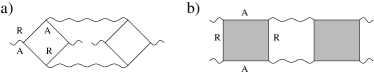
Figure 1: (a), (b) Diagrams contributing to mesoscopic sample-to-sample fluctuations of superconducting density. Solid lines represent disorder averaged Green function; short wavy lines stand for current vertexes. The shaded regions in (b) indicate appropriately renormalized Hikami boxes, see text and Fig. 4. Long wavy lines stand for diffuson/Cooperon impurity ladders $\mathcal{D}(x_{1},x_{2})$, see discussion after Eq. (19).

A similar correlator to $\mathcal{F}$ appears in the variance of conductance fluctuations in the normal metal for which a perturbation theory in $k_{F}\ell\gg 1$ was developed and used extensivelyLee et al. (1987). The main order contribution in this perturbation series may be written in terms of the diagrams shown in Fig. 1. In the case of a superconductor the diagrams will have a similar form.

It is instructive therefore to compare expressions Eqs. (8, 9, 10) with the normal case. The amplitude of normal state conductance fluctuations contains only the diagrams shown in Fig. 1. It has been shown rigorouslyBaranger and Stone (1989) that dissipative normal state conductance is fully determined by products of one retarded and one advanced Green functions averaged together $G^{R}G^{A}$, compare Eq. (8). Therefore expanding the normal state analog of the Eq. (8) in terms of $G^{R}$ and $G^{A}$ (in other words the formula for conductance) the products of two retarded or two advanced Green functions in Eq. (8) that describe non-dissipative diamagnetic currents vanish. A normal state analog of the correlator $\mathcal{F}$ in Eq. (10) contains therefore only the averages of the type $\langle G^{R}G^{A}G^{R}G^{A}\rangle$ resulting in the diagrams in Fig. 1 being the only diagrams contributing to conductance fluctuations. In contrast to the normal phase, the superfluid density is a thermodynamic property of a superconductor and despite Anderson theorem relating it to the normal state conductivity the same arguments do not apply. One has to be cautious and take into account a number of additional diagrams shown in Fig. 2 which vanish in a normal state yet give non-zero contribution in the superconducting phase. These diagrams originate form the terms of the form $G^{R}G^{R}$ in the superconducting density Eq. (8). A more detailed discussion of the standard procedure of constructing the diagramatic perturbation theory can be found in Appendix A.

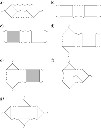
Figure 2: Diagrams obtained originating from the contributions of the form $G^{R}(x_{1},x_{2})G^{R}(x_{2},x_{1})$ to each of the superfluid densities Eq. (8) in the correlator Eq. (9). These diagrams cancel in the case of normal state conductance calculation yet contribute to the superfluid density.

The diagrams in Figs. 1 and 2 can be simplified in the standard wayLee et al. (1987); Akkermans and Montambaux (2007) by identifying two types of blocks characterized by distinct length scales: the mean free path $\ell$ and the coherent diffusion length scale $\zeta\gg\ell$. For the diagram in Fig. 1(a) such separation is done as follows,

$$\mathcal{F}_{1a}\equiv W^{2}\int\prod_{i=1}^{4}dx_{i}j(x_{1},x_{2})j(x_{3},x_{4})\mathcal{D}(x_{1},x_{3})\mathcal{D}(x_{4},x_{2})$$

$$\times\exp(i\xi_{1}t_{1}-i\xi_{3}t_{3}+i\xi_{4}t_{4}-i\xi_{2}t_{2}),$$ (11)

where $x_{i}\equiv(\mathbf{r_{i}},t_{i})$. We introduced the ’Hikami boxes’ $j(x_{1},x_{2})$ and the diffuson/Cooperon propagators $\mathcal{D}(x_{1},x_{2})$, see Fig. 1. In the main order in $p_{F}\ell\gg 1$ and $\zeta/\ell\gg 1$ these blocks can be averaged over disorder independently of each other.

The diffusion propagator is defined as a joint average of two Green functions $\mathcal{D}(x_{1},x_{2})=\frac{1}{2\pi\nu\tau^{2}}\langle G^{R}(x_{1},x_{2})G^{A}(x_{2},x_{1})\rangle$ and describes the long-range coherent diffusion of electrons on the scales $|\mathbf{r_{1}}-\mathbf{r_{2}}|\gg\ell$Akkermans and Montambaux (2007). The diffuson propagators are represented diagramatically by impurity ladders of diffuson and Cooperon typeAkkermans and Montambaux (2007) and satisfy Dyson-like equations Figs. 3(a). In the diffusive regime Figs. 3(a) reduces to the standard diffusion equation. To model a realistic conductor this diffusion equation has to be supplemented with boundary conditions. We set $\mathcal{D}=0$ at the contacts and $\nabla\mathcal{D}=0$ at the surface of the wire. The diffusion propagators can be written in terms of the eigenmodes of the diffusion equation $\Phi_{\mathbf{q}}(\mathbf{r})=\sqrt{\frac{2^{3}}{L_{x}L_{y}L_{z}}}\sin q_{x}x\cos q_{y}y\cos q_{z}z$, $\mathbf{q}=\left[\frac{\pi n_{x}}{L_{x}},\frac{\pi n_{y}}{L_{y}},\frac{\pi n_{z}}{L_{z}}\right]$, $n_{x}=1,2,..$ $n_{y},n_{z}=0,1,2...$,

$$\mathcal{D}(t,\mathbf{r,r^{\prime}})=\frac{1}{2\pi\nu\tau^{2}}\sum_{q}e^{-Dq^{2}t}\Phi_{q}(\mathbf{r})\Phi_{q}(\mathbf{r^{\prime}}),$$ (12)

where $t\geq 0$ stands for the diffusion time, $D$ is the diffusion coefficient for electrons and $\nu$ is the density of electronic states. Averaging over the wire volume in Eq. (11) of the product of orthogonal eigenfunctions $\Phi_{\mathbf{q}}(\mathbf{r})$ gives rise to the momentum conservation condition (and this is true also for all other diagrams). As a result all diffusion propagators in each diagram in Figs. 1, 2 have the same momentum $q$. Sums over $q$ may be approximated by integral in the case $\zeta/L_{i}\ll 1,\,i=x,\,y,\,z$,

$$\sum_{q}\rightarrow\frac{\Omega_{d}}{\pi^{d}\zeta^{d}}\int_{0}^{\infty}dk_{i},$$ (13)

where $\Omega_{d}=\left[V,\,L_{z}L_{y},\,L_{z}\right]$ for $d=3,2,1$. We define dimensionality $d$ of the sample with respect to the coherence length, i.e. $d=3$ corresponds to $L_{x},\,L_{y},\,L_{z}\gg\zeta$, $d=2$ corresponds to $L_{x},\,L_{z}\gg\zeta>L_{y}$ and $d=1$ corresponds to $L_{z}\gg\zeta>L_{x},\,L_{y}$.

The following relation will be useful,

$$\sum_{q}q^{2m}e^{-Dq^{2}t}\approx\frac{\kappa_{m}}{2^{d}\pi^{d/2}}\frac{1}{(t\Delta){}^{d/2+m}}\frac{\Omega_{d}}{\zeta^{d}}\frac{1}{\zeta^{2m}},$$ (14)

where $m=0,1,2$ and $\kappa_{m}=1,\frac{1}{2},\frac{3}{4}$ respectively. In the absence of magnetic fields the Cooperon and diffuson propagators are identical and we will not distinguish them in the following, instead including a factor of $2$ in front of all the diagrams.

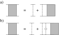
Figure 3: Dyson equations for diffusons/Cooperons (shaded regions) in time reversal symmetric case. Vertical dashed lines stand for the disorder correlator $\langle u(\mathbf{r})u(\mathbf{r^{\prime}})\rangle=\frac{1}{2\pi\nu\tau}\delta(\mathbf{r-r^{\prime}})$, solid lines correspond to disorder averaged Green functions. (a) Corresponds to static impurity configuration. (b) Corresponds to the case when a fraction of impurities have moved between different measurements. The additional “diamond” vertex corresponds to the correlator $\langle\left(u_{\mathbf{r_{i}}+\delta\mathbf{r}}-u_{\mathbf{r_{i}}}\right)u_{\mathbf{r_{i}}}\rangle$.

The second type of blocks that we introduced in Eq. (11) are Hikami boxes $j(x_{1},x_{2})$. There are four types shown in Fig. 4, where straight lines represent disorder averaged Green functions. $j(x_{1},x_{2})$ decays exponentially on the short length scales of the order of the mean free path $|r|\sim\ell\ll L_{x},\,L_{y}$ and therefore can be approximated by a delta function $j(x_{1},x_{2})\approx j_{0}\delta(x_{1}-x_{2})$. The constant factor $j_{0}$ can be calculated in momentum space using disorder averaged Green functions. The result of this calculation for each of the vertexes in Fig. 4(a)-(d) reads,

$$j_{a}\approx\frac{4\pi\nu\tau^{3}p_{F}^{2}}{d},$$ (15)

$$j_{b}\approx\frac{2\pi\nu\tau^{3}p_{F}^{2}}{d},$$ (16)

$$j_{c}\approx-\frac{2\pi\nu\tau^{3}p_{F}^{2}}{d},$$ (17)

$$j_{d}^{\alpha}\approx\pm\frac{4\pi\nu\tau^{3}p_{F}^{2}}{d}\frac{q_{\alpha}}{m},$$ (18)

where the expression for the last vertex depends explicitly on the momentum of the diffusion eigenmodes $\mathbf{q}$.

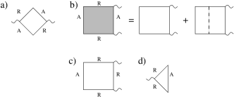
Figure 4: Four types of Hikami boxes appearing in the diagrams in Figs. 1 and 2.

Using the short range character of the current vertexes we simplify Eq. (11) for the diagram in Fig. 1 (a),

$$\mathcal{F}_{1a}\equiv W^{2}j_{a}^{2}\int d\mathbf{r}d\mathbf{r^{\prime}}dtdt^{\prime}\mathcal{D}(t,\mathbf{r},\mathbf{r^{\prime}})\mathcal{D}(t^{\prime},\mathbf{r^{\prime}},\mathbf{r})$$

$$\times\exp(-i(\xi_{1}-\xi_{4})t-i(\xi_{3}-\xi_{2})t^{\prime}).$$ (19)

Note that all energy dependence in the above expression is contained in Fourier factors. As a result after substituting Eq. (19) into Eq. (9) we can take integrals with respect to energy in Eq. (9). The expression for the diagram in Fig. 1(a) therefore can be rewritten using Eqs. (9,19,14),

$$\langle\delta S^{2}\rangle_{1a}=\frac{2^{-d}\pi^{-\frac{d}{2}}W^{2}j_{a}^{2}\Delta^{2}}{(2\pi\nu\tau^{2})^{2}}\frac{\Omega_{d}}{\zeta^{d}}\int_{0}^{\infty}\frac{d\lambda d\lambda^{\prime}\left(\Theta_{\lambda+\lambda^{\prime}}^{(-)}\right)^{2}}{(\lambda+\lambda^{\prime})^{d/2}},$$ (20)

and introducing the Fourier integral,

$$\Theta_{\lambda+\lambda^{\prime}}^{(-)}\equiv\frac{1}{\Delta}\int d\xi d\xi^{\prime}\mathcal{L}_{\xi\xi^{\prime}}e^{i\xi\frac{\lambda}{\Delta}-i\xi^{\prime}\frac{\lambda^{\prime}}{\Delta}}=-2\pi\int_{\lambda+\lambda^{\prime}}^{\infty}dxK_{0}(x),$$ (21)

where $K_{n}(x),\,n=0,1,2,..$ is the modified Bessel functionGradshteyn and Ryzhik (1980) and we introduced a dimensionless time $\lambda\equiv t\Delta$ measured in units of $1/\Delta$. See Appendix B for details of Fourier integration. Note that the integral over $\lambda,\,\lambda^{\prime}$ in the right hand side of Eq. (20) is dimensionless and therefore simply represents a numerical coefficient.

It is instructive to show the calculation of the diagram in Fig. 1(b),

$$j_{b}^{2}\int d\mathbf{r}d\mathbf{r^{\prime}}\mathcal{D}(t,\mathbf{r},\mathbf{r^{\prime}})\mathcal{D}(t^{\prime},\mathbf{r^{\prime}},\mathbf{r}))$$

$$\times\exp(-i(\xi_{1}-\xi_{4})t-i(\xi_{1}-\xi_{4})t^{\prime}).$$

Including the coherence factors in Eq. (9) and using Eq. (14) we get,

$$\langle\delta S^{2}\rangle_{1b}=\frac{2^{-d}\pi^{-\frac{d}{2}}W^{2}j_{b}^{2}\Delta^{2}}{(2\pi\nu\tau^{2})^{2}}\frac{\Omega_{d}}{\zeta^{d}}\int_{0}^{\infty}\frac{d\lambda d\lambda^{\prime}}{(\lambda+\lambda^{\prime})^{d/2}}\left(\Theta_{\lambda+\lambda^{\prime}}^{(0)}\right)^{2},$$ (22)

where crucially the Fourier integral has a distinct form from that in Eq. (21),

$$\Theta_{\lambda+\lambda^{\prime}}^{(0)}\equiv\frac{1}{\Delta}\int d\xi d\xi^{\prime}\mathcal{L}_{\xi\xi^{\prime}}e^{i\xi\frac{(\lambda+\lambda^{\prime})}{\Delta}}$$

$$=-\pi\int_{\lambda+\lambda^{\prime}}^{\infty}dx\left(K_{0}(x)+\frac{1-xK_{1}(x)}{x^{2}}\right).$$ (23)

Note that here we switched to dimensionless time $\lambda\equiv\Delta t$. The details of the integration are shown in Appendix B. The rest of the diagrams can be computed in the analogous way noting that the diagrams in Fig. 2 contain the third type of the Fourier transform of the coherence factor,

$$\Theta_{\lambda+\lambda^{\prime}}^{(+)}\equiv\frac{1}{\Delta}\int d\xi d\xi^{\prime}\mathcal{L}_{\xi\xi^{\prime}}e^{i\xi\frac{\lambda}{\Delta}+i\xi^{\prime}\frac{\lambda^{\prime}}{\Delta}}$$

$$=-2\pi\int_{\lambda+\lambda^{\prime}}^{\infty}dx\frac{1-xK_{1}(x)}{x^{2}}.$$ (24)

Note that the long range asymptotic, $x\gg 1$, of the Bessel function is proportional to an exponent $K_{\nu}(x)\approx\sqrt{\frac{\pi}{2x}}e^{-x}$. This means that the Fourier transform of the coherence factor Eq. (6) $\Theta_{\lambda}^{(-)}\sim e^{-\lambda}$ determines the roughly exponential phase relaxation in the diagram in Fig. 1(a), Eq. (20). This diagram corresponds to the fluctuations in the transmission coefficient of electrons in the superconductor. In contrast, in the diagram in Fig. 1(b), Eq. (22), $\Theta_{\lambda}^{(0)}\sim\frac{1}{\lambda}$ and therefore the coherent diffusion is only suppressed by a slow power law phase relaxation rather than an exponent. An analogous slow relaxation of diffusion modes is described by the diagrams in Fig. 2. Note that the non-exponential relaxation of the diffusion modes is precisely the reason why the diagrams in Fig. 2 give non-zero contribution in contrast to the normal metal case. This can be seen by replacing each of the Fourier integrals $\Theta_{\lambda}^{(-)},\,\Theta_{\lambda}^{(0)},\,\Theta^{(+)}$ with an exponent $e^{-\lambda}$ in which case the sum of the diagrams in Fig. 2 vanishes, see Appendix A for details. The consequences of non-exponential relaxation is two-fold: (i) due to both the contribution of the numerous additional diagrams and slow-decaying non-exponential integrands the amplitude of the superfluid density fluctuations is enhanced; (ii) as we will see in the following the noise amplitude acquires non-linear dependence on the effective impurity strength in one and two dimensions.

Summing all the diagrams in Figs. 1,2 including the appropriate symmetry factors, see Appendix A, we arrive at,

$$\frac{\langle\delta S^{2}\rangle}{S^{2}}=C_{d}\frac{1}{(p_{F}\ell)^{4}}\frac{\zeta^{4-d}\ell^{2}\Omega_{d}}{V^{2}},$$ (25)

$$C_{d}\equiv 2^{1-d}9\pi^{-d/2}\left(\mathcal{I}^{RA}+2\mathcal{I}^{RR}\right).$$ (26)

where $\Omega_{d}=\left[V,L_{z}L_{y},L_{z}\right]$ for $d=3,2,1$. The explicit form of the integrals in Eq. (26) reads,

$$\mathcal{I}^{RA}=\int_{0}^{\infty}d\lambda_{1}d\lambda_{2}\frac{\left(\Theta_{\lambda_{1}+\lambda_{2}}^{-}\right)^{2}+\frac{1}{2}\left(\Theta_{\lambda_{1}+\lambda_{2}}^{0}\right)^{2}}{(\lambda_{1}+\lambda_{2})^{d/2}}A_{\lambda_{1}+\lambda_{2}},$$ (27)

corresponding to the contribution of the diagrams in Fig. 1, and

$$\mathcal{I}^{RR}=\int_{0}^{\infty}d\lambda_{1}d\lambda_{2}\frac{\left(\left(\Theta_{\lambda_{1}+\lambda_{2}}^{+}\right)^{2}+\frac{3}{2}\Theta_{\lambda_{1}+\lambda_{2}}^{+}\Theta_{\lambda_{1}+\lambda_{2}}^{0}\right)A_{\lambda_{1}+\lambda_{2}}}{(\lambda_{1}+\lambda_{2})^{d/2}}$$

$$-2\int_{0}^{\infty}d\lambda_{1}d\lambda_{2}d\lambda_{3}\frac{\left(\Theta_{\lambda_{1}+\lambda_{2}+\lambda_{3}}^{+}\right)^{2}A_{\lambda_{1}+\lambda_{2}+\lambda_{3}}}{(\lambda_{1}+\lambda_{2}+\lambda_{3})^{d/2+1}}$$

$$-2\int_{0}^{\infty}d\lambda_{1}d\lambda_{2}d\lambda_{3}\frac{\Theta_{\lambda_{1}+\lambda_{2}+\lambda_{3}}^{+}\Theta_{\lambda_{1}+\lambda_{2}+\lambda_{3}}^{0}A_{\lambda_{1}+\lambda_{2}+\lambda_{3}}}{(\lambda_{1}+\lambda_{2}+\lambda_{3})^{d/2+1}}$$

$$+\int_{0}^{\infty}d\lambda_{1}d\lambda_{2}d\lambda_{3}d\lambda_{4}\frac{9\left(\Theta_{\lambda_{1}+\lambda_{2}+\lambda_{3}+\lambda_{4}}^{+}\right)^{2}A_{\lambda_{1}+\lambda_{2}+\lambda_{3}+\lambda_{4}}}{(\lambda_{1}+\lambda_{2}+\lambda_{3}+\lambda_{4})^{d/2+2}},$$ (28)

corresponding to the contribution of the diagrams in Fig. 2. The factor $A_{\lambda}=1$ in Eq. (25). We estimate the coefficients in Eq. (25) by numerically taking the integrals in Eqs. (27, 28) $C_{3}\approx 25,C_{2}\approx 60,C_{1}\approx 200$.

III Noise amplitude

A model of tunneling two level (bistable) defect, i.e. an impurity fluctuating between two spatial positions, is used to describe noise in a wide range of materials. For simplicity we use this model to give a precise meaning to the amplitude of the noise calculated here. All of the results can be easily generalized for a more generic dynamics of impurities Al’tshuler and Spivak (1985). In the presence of a single bistable defect superfluid response demonstrates significant fluctuations. The noise amplitude for a single defect is given by the correlator,

$$\langle\delta S_{\delta\mathbf{r}}^{2}\rangle=\langle\delta S^{2}\rangle-\langle\delta S_{\mathbf{r_{i}+\delta}\mathbf{r}}\delta S_{\mathbf{r_{i}}}\rangle.$$ (29)

The first term on the right hand side of Eq. (29) is simply the fluctuation amplitude Eq. (25), $\delta S\equiv S-\langle S\rangle$. The second term corresponds to the diagrams in Figs. 1 and 2 with one of the response kernels $\delta S_{\mathbf{r_{i}+\delta}\mathbf{r}}$ containing the disorder configuration with one defect shifted from $\mathbf{r_{i}}$ by a distance $\mathbf{\delta r}$, and the other $\delta S_{\mathbf{r_{i}}}$ containing the bistable defect in its original position $\mathbf{r_{i}}$. This shift introduces an effective dephasing rate cutting off the diffusion modes. To show this we recalculate the diffuson/Cooperon in the presence of the shifted bistable defect. The Dyson equation for the diffuson/Cooperon has to be modified by including an additional vertex shown in Fig. 3(b) as an impurity line with a diamondFeng et al. (1986); Fal’ko and Khmel’nitskii (1990). This new vertex corresponds to the correlator $\langle\left(u_{\mathbf{r_{i}}+\delta\mathbf{r}}-u_{\mathbf{r_{i}}}\right)u_{\mathbf{r_{i}}}\rangle$. It is obtained in the perturbation expansion in the small parameter, $\langle\left(u_{\mathbf{r_{i}}+\delta\mathbf{r}}-u_{\mathbf{r_{i}}}\right)u_{\mathbf{r_{i}}}\rangle/\langle u_{\mathbf{r_{i}}}u_{\mathbf{r_{i}}}\rangle$. In momentum space the last term in Fig. 3(c) reads,

$$u_{0}^{2}\int\frac{d\mathbf{p}d\mathbf{p^{\prime}}}{(2\pi)^{6}}|G_{\mathbf{p}}^{R}|^{2}|G_{\mathbf{p^{\prime}}}^{A}|^{2}\left(\cos\left[\mathbf{(p-p^{\prime})\delta r}\right]-1\right)\mathcal{D}(\mathbf{q}),$$ (30)

where we keep only the main contribution in the gradient expansion of the diffusion mode. This gives,

$$\left(-i\omega+Dq^{2}+\tau_{eff}^{-1}\right)\mathcal{D}(q)=1,$$ (31)

$$\tau_{eff}^{-1}=\frac{1}{\tau}\alpha(k_{F}\delta r),$$ (32)

$$\alpha(k_{F}\delta r)\equiv\left(1-\frac{\sin^{2}\left(k_{F}\delta r/2\right)}{(k_{F}\delta r/2)^{2}}\right).$$ (33)

In the presence of more than one thermally activated defect their contributions simply add up for small enough concentration of such defects $\gamma_{T}$,

$$\tau_{eff}^{-1}\approx\gamma_{T}\frac{1}{\tau}\langle\alpha(k_{F}\delta r)\rangle,$$ (34)

which includes an average over characteristics of bistable defects $\langle\alpha(k_{F}\delta r)\rangle$. For defects characterized by $k_{F}\delta r\gg 1$, $\langle\alpha(k_{F}\delta r)\rangle\approx 1$. The effect of bistable defects on the vertex parts of the diagrams $j(r_{1},r_{2})$ is small as $\ell/\zeta$, and therefore we neglect it in the following. The main order amplitude of the noise in the superfluid density Eq. (29) is given by the same diagrams in Figs. 1, 2. However, in the case of the second term in Eq. (29) we need to include the dephasing effect of thermally activated defects Eq. (34). The result is,

$$\delta_{K}^{2}=\widetilde{C}_{d}\frac{1}{(p_{F}\ell)^{4}}\frac{\zeta^{4-d}\ell^{2}\Omega_{d}}{V^{2}},$$ (35)

$$\widetilde{C}_{d}\equiv 9\pi^{-d/2}2^{1-d}\left(\mathcal{I}^{RA}(\tau_{eff})+2\mathcal{I}^{RR}(\tau_{eff})\right),$$ (36)

where the integrals $\mathcal{I}^{RA}(\tau_{eff}),\,\mathcal{I}^{RR}(\tau_{eff})$ are given by Eq. (27, 28) with the factor $A_{t}$ modified to include the effect of bistable defects,

$$A_{\lambda}\equiv 1-e^{-\lambda/(\Delta\tau_{eff})}.$$ (37)

The first and the second term in Eq. (37) correspond to the first and the second terms in Eq. (29). The factor $\Omega_{d}$ has the same meaning as in Eq. (25).

The amplitude of the noise in $d=3$ can be estimated by expanding the exponent in Eq. (37), $A_{\lambda}\approx\frac{\lambda}{\Delta\tau_{eff}}$, resulting in,

$$\delta_{K}^{2}\approx 60\gamma_{T}\frac{1}{(p_{F}\ell)^{4}}\frac{\zeta^{3}}{V},$$ (38)

where we took the integrals in Eq. (36) numerically to estimate the value of the coefficient.

In lower dimensions the simple expansion of the factor in Eq. (37) is not possible since the integral over $t$ diverges. Instead we keep only the main asymptotic contribution in the parameter $\Delta\tau_{eff}=3\zeta^{2}/(\gamma_{T}\ell^{2})\gg 1$ which gives,

$$\delta_{K}^{2}=\frac{297}{4\pi}\gamma_{T}\log\left[\frac{3\zeta^{2}}{\gamma_{T}\ell^{2}}\right]\frac{1}{(p_{F}\ell)^{4}}\frac{\zeta^{4}}{VL_{y}},$$ (39)

in effective two dimensional superconductor, $L_{y}\lesssim\zeta\ll L_{x},L_{z}$, and

$$\delta_{K}^{2}=99\left(3\gamma_{T}\right)^{\frac{1}{2}}\frac{1}{(p_{F}\ell)^{4}}\frac{\zeta^{4}\ell}{VS_{\perp}},$$ (40)

in effective one dimension, $L_{x},L_{y}\lesssim\zeta\ll L_{z}$. The results Eqs. (38-40) are valid only in the limit of very small relative concentration of bistable defects $\gamma_{T}\ll 1$ such that the noise amplitude is much smaller than the sample-to-sample fluctuation Eq. (25) which sets the upper limit on the noise amplitude. At high concentration of fluctuating defects the noise amplitude saturates at the value of sample-to-sample fluctuations Eq. (25).

IV Conclusion

We have performed the detailed analysis of kinetic inductance fluctuations caused by motion of impurities in the superconductor and enhanced by the mesoscopic quantum interference. We found that the effect is closely related to the universal conductance fluctuations in normal metals with an important distinction that the superconducting coherence length determines the scale of coherent diffusion, in contrast to the inelastic scattering length in the normal metal. We found that the phase relaxation in superconductors has slow non-exponential character which results in the enhanced amplitude of the noise and non-linear scaling of the amplitude with the density of fluctuating impurities. Our estimates of the magnitude of the noise suggest that the effect is likely to dominate inductance noise in small devices. Experimentally, the interference contribution to the inductance noise can be unambiguously identified by driving supercurrents close to critical in magnitude through the wire. In presence of strong supercurrent the superconducting order parameter phase changes by $2\pi$ on the scale of the coherence length which results in strong suppression of the quantum interference and therefore the noise amplitude.

The upper limit of the noise amplitude is given by the mesoscopic fluctuation amplitude. We estimate this amplitude for an Al wire with dimensions $100\textrm{nm}\times 100\textrm{nm}\times 10\mu\textrm{m}$ using Eq. (25), $\frac{\sqrt{\left\langle\delta K^{2}\right\rangle}}{K}\sim 10^{-5}$.

In normal state metals the mesoscopic noise amplitude was found to be roughly temperature independent. This was attributed to a rough cancellation of the temperature dependence of the density of thermally activated defects $\gamma_{T}\propto T$ and the temperature smearing of the mesoscopic fluctuation which roughly suppresses the amplitude as $\propto 1/T$ Birge et al. (1989). In contrast, in the very low temperature regime of transport in disordered superconductors considered here the mesoscopic noise is limited by the superconducting coherence length which demonstrates very weak temperature dependence away from the transition temperature. As a result we expect the mesoscopic noise in the kinetic inductance of disordered superconducting wires in presence of thermally activated impurity dynamics to scale linearly with with temperature $\propto T$ in the effective $d=3$ case and $\propto T\log T$ in $d=2$ and $\propto\sqrt{T}$ in $d=1$. This prediction could be tested experimentally in superconducting thin films and wires.

Appendix A Details of the diagrams evaluation

Fig.	1a	1b	2a	2b	2c	2d	2e	2f	2g
factor	2	4	4	8	8	8	16	8	12

Table 1: Combinatorial factors corresponding to diagrams of different topologies shown in Fig. 1, 2 contributing to the kinetic inductance fluctuations and the noise amplitude.

Fluctuations of the superfluid response are given by the disorder, spatial and energy average of a correlator $\mathcal{F}$ (see Eq. (9)) of four matrix elements of the current operator. This correlator can be rewritten in terms of four imaginary parts of the exact Green functions, see Eq. (8),

$$\mathcal{F}\propto\left\langle\Delta G\overleftrightarrow{\nabla}\overleftrightarrow{\nabla^{\prime}}\Delta\overline{G}\Delta G\overleftrightarrow{\nabla}\overleftrightarrow{\nabla^{\prime}}\Delta\overline{G}\right\rangle$$ (41)

The diagrams in Figs. 1, 2 are constructed by pairing Green functions to form diffuson and Cooperon ladders, which are products of one retarded and one advanced Green functions averaged over disorder $\left\langle G^{R}G^{A}\right\rangle$. All possible such connections give rise to the diagrams in Figs. 1, 2. In particular, the average of the form,

$$\left\langle G^{R}\overleftrightarrow{\nabla}\overleftrightarrow{\nabla^{\prime}}G^{A}G^{R}\overleftrightarrow{\nabla}\overleftrightarrow{\nabla^{\prime}}G^{A}\right\rangle$$ (42)

gives rise to the two diagrams shown in Fig. 1(a),(b). These are the diagrams that correspond to normal state conductance fluctuationsLee et al. (1987); Akkermans and Montambaux (2007); Baranger and Stone (1989). The averages of the form,

$$\left\langle G^{A}\overleftrightarrow{\nabla}\overleftrightarrow{\nabla^{\prime}}G^{A}G^{R}\overleftrightarrow{\nabla}\overleftrightarrow{\nabla^{\prime}}G^{R}\right\rangle$$ (43)

give rise to the diagrams in Figs. 2(a),(b),(d),(f) and (g). Finally, the averages of the form,

$$-\left\langle G^{R}\overleftrightarrow{\nabla}\overleftrightarrow{\nabla^{\prime}}G^{A}G^{R}\overleftrightarrow{\nabla}\overleftrightarrow{\nabla^{\prime}}G^{R}\right\rangle$$ (44)

give rise to the diagrams shown in Fig. 2(c) and (e). Crucially, the latter expression comes with a different sign from expanding the expression in Eq. (41).

Each diagram in Figs. 1 and 2 comes with a different “combinatorial factor” reflecting the number of times it occurs in the perturbation expansion of $\left\langle\delta S^{2}\right\rangle$. This factor counts the number of ways to choose pairs of $\langle G^{R}G^{A}\rangle$ such that the two Green functions are parts of different superfluid density loops. The corresponding factors are summarized in Table 1.

In the case of mesoscopic fluctuations of the normal state conductance it has been shownBaranger and Stone (1989) that only the diagrams constructed from $G^{R}G^{A}$ loops (Eq. (42) and Fig. 1) give non-zero contribution. Since the symmetry factors and the Hikami boxes in all of the diagrams constructed using $G^{R}G^{R}$ loops (Fig. 2) are the same as in the normal state we expect exact cancellation of the contribution of such diagrams to the normal state conductance fluctuations. To very that this contribution indeed vanishes we set all Fourier transformed coherence factors to be equal to an exponent $\Theta_{\lambda}^{(0)},\Theta_{\lambda}^{(+)},\Theta_{\lambda}^{(-)}\rightarrow e^{-\lambda/\tau_{\varphi}}$ describing the effect of decoherence due to inelastic electron-electron or electron-phonon collisions operational in the normal state. The resulting sum of the integrals vanishes exactly $\mathcal{I}{}^{RR}(\tau_{\varphi})=0$. Note that the non-exponential decay of $\Theta_{\lambda}^{(0)},\Theta_{\lambda}^{(+)},\Theta_{\lambda}^{(-)}$ is precisely the reason for non-vanishing contribution of the diagrams in Fig. 2 to the superfluid response fluctuations.

Appendix B Fourier integrals of the coherence factor

B.1 First type integral

In the following we calculate the Fourier integral,

$$\Theta_{t+t^{\prime}}^{(-)}=\frac{1}{\Delta}\int_{-\infty}^{\infty}d\xi d\xi^{\prime}\delta\mathcal{L}_{\xi\xi^{\prime}}e^{-i\xi t+i\xi^{\prime}t^{\prime}},$$ (45)

in Eq. (20), see also Ref. Bardeen et al., 1957. Note that in this appendix we perform the calculations using the real time as opposed to the dimensionless time $\lambda$. We introduce the latter at the end of the calculation. We introduce notations symmetric with respect to $\xi\rightarrow-\xi$,

$$\mathcal{L}_{\xi\xi^{\prime}}=\frac{1}{2}\frac{F(\xi)-F(\xi^{\prime})+\xi\xi^{\prime}\left[G(\xi)-G(\xi^{\prime})\right]}{\xi^{2}-\xi^{\prime 2}}.$$ (46)

where the symmetric functions $F(\xi)=F(-\xi)$ and $G(\xi)=G(-\xi)$ are defined as,

$$F(\xi)=\left(E+\frac{\Delta^{2}}{E}\right)\left[1-2f(E)\right]-\xi\left[1-2f(\xi)\right],$$ (47)

$$G(\xi)=\frac{1}{E}\left[1-2f(E)\right]-\frac{1}{\xi}\left[1-2f(\xi)\right],$$ (48)

note that $f(-\xi)=1-f(\xi)$.

Using Eqs. (46,47,48) we write,

$$\Theta_{t+t^{\prime}}^{(-)}=\frac{2}{\Delta}\int_{0}^{\infty}d\xi d\xi^{\prime}\frac{\cos\xi t\cos\xi^{\prime}t^{\prime}\left[F(\xi)-F(\xi^{\prime})\right]}{\xi^{2}-\xi^{\prime 2}}$$

$$+\frac{2}{\Delta}\int_{0}^{\infty}d\xi d\xi^{\prime}\frac{\xi\xi^{\prime}\sin\xi t\sin\xi^{\prime}t^{\prime}\left[G(\xi)-G(\xi^{\prime})\right]}{\xi^{2}-\xi^{\prime 2}}$$ (49)

We replace the integral in the above expression by two principal value (at point $\xi=\xi^{\prime}$) integrals,

$$A_{1}=2\lim_{a\rightarrow 0,b\rightarrow\infty}\mathcal{P}^{\prime}\int_{a}^{b}\int_{a}^{b}d\xi d\xi^{\prime}\frac{\cos\xi t\cos\xi^{\prime}t^{\prime}F(\xi)}{\xi^{2}-\xi^{\prime 2}},$$ (50)

$$A_{2}=2\lim_{a\rightarrow 0,b\rightarrow\infty}\mathcal{P}^{\prime}\int_{a}^{b}\int_{a}^{b}d\xi d\xi^{\prime}\frac{\xi\xi^{\prime}\sin\xi t\sin\xi^{\prime}t^{\prime}G(\xi)}{\xi^{2}-\xi^{\prime 2}}.$$ (51)

Since $F(\xi)\rightarrow 0$ as $\xi\rightarrow\infty$ the value of the integral does not depend on the way the upper limit is approached. Therefore we can set $b\rightarrow\infty$ right away. Care must be taken with the lower limit, for the integral in Eq. (50),

$$\int_{a}^{\infty}d\xi^{\prime}\frac{\cos\xi^{\prime}t^{\prime}}{\xi^{2}-\xi^{\prime 2}}=\int_{0}^{\infty}d\xi^{\prime}\frac{\cos\xi^{\prime}t^{\prime}}{\xi^{2}-\xi^{\prime 2}}-\int_{0}^{a}d\xi^{\prime}\frac{1}{\xi^{2}-\xi^{\prime 2}},$$ (52)

where in the last expression we assumed $a$ small enough so that $\cos\xi^{\prime}t\approx 1$. We evaluate the second term in Eq. (52),

$$\int_{0}^{a}d\xi^{\prime}\frac{1}{\xi^{2}-\xi^{\prime 2}}=\frac{1}{2\xi}\ln\frac{\xi+a}{\xi-a},$$ (53)

which is possible since $\xi>a$. In the first term in Eq. (52) the principal value integral gives,

$$\mathcal{P}^{\prime}\int_{0}^{\infty}d\xi^{\prime}\frac{\cos\xi^{\prime}t^{\prime}}{\xi^{2}-\xi^{\prime 2}}=\frac{\pi}{2}\frac{\sin\xi t^{\prime}}{\xi},$$ (54)

A similar integral in Eq. (51) gives,

$$\mathcal{P}^{\prime}\int_{0}^{\infty}d\xi^{\prime}\frac{\xi^{\prime}\sin\xi^{\prime}t^{\prime}}{\xi^{2}-\xi^{\prime 2}}=-\frac{\pi}{2}\cos\xi t^{\prime}.$$ (55)

So that

$$A_{1}+A_{2}=-\lim_{a\rightarrow 0}\int_{a}^{\infty}\frac{d\xi}{\xi}F(\xi)\ln\frac{\xi+a}{\xi-a}$$ (56)

$$+2\lim_{a\rightarrow 0}\int_{a}^{\infty}d\xi\cos\xi tF(\xi)\frac{\pi}{2}\frac{\sin\xi t^{\prime}}{\xi}$$ (57)

$$+2\lim_{a\rightarrow 0}\int_{a}^{\infty}d\xi\xi\sin\xi tG(\xi)\left(-\frac{\pi}{2}\cos\xi t^{\prime}\right).$$ (58)

Similar expressions arise in Eq. (49) where the integral over $\xi$ is taken first. Combining all the results we get,

$$\Theta_{t+t^{\prime}}^{(-)}=-\frac{2}{\Delta}\lim_{a\rightarrow 0}\int_{a}^{\infty}\frac{d\xi}{\xi}F(\xi)\ln\frac{\xi+a}{\xi-a}$$ (59)

$$+\frac{\pi}{\Delta}\lim_{a\rightarrow 0}\int_{a}^{\infty}d\xi F(\xi)\cos\xi t\frac{\sin\xi t^{\prime}}{\xi}$$ (60)

$$-\frac{\pi}{\Delta}\lim_{a\rightarrow 0}\int_{a}^{\infty}d\xi\xi G(\xi)\sin\xi t\cos\xi t^{\prime}$$ (61)

$$+\frac{\pi}{\Delta}\lim_{a\rightarrow 0}\int_{a}^{\infty}d\xi F(\xi)\cos\xi t^{\prime}\frac{\sin\xi t}{\xi}$$ (62)

$$-\frac{\pi}{\Delta}\lim_{a\rightarrow 0}\int_{a}^{\infty}d\xi\xi G(\xi)\sin\xi t^{\prime}\cos\xi t,$$ (63)

where we have replaced $\xi^{\prime}$ with $\xi$ in the last two terms. Simplifying this expression we get,

$$\Theta_{t+t^{\prime}}^{(-)}=-\frac{2}{\Delta}\lim_{a\rightarrow 0}\int_{a}^{\infty}\frac{d\xi}{\xi}F(\xi)\ln\frac{\xi+a}{\xi-a}$$ (64)

$$+\frac{\pi}{\Delta}\lim_{a\rightarrow 0}\int_{a}^{\infty}d\xi\left[F(\xi)-\xi^{2}G(\xi)\right]$$ (65)

$$\times\frac{\cos\xi t^{\prime}\sin\xi t+\sin\xi t^{\prime}\cos\xi t}{\xi}.$$ (66)

In the first term in the latter, as we take the limit we can take $F(\xi)\rightarrow F(0)=2\Delta\left[1-2f(\Delta)\right]$ and calculate the integral,

$$\int_{1}^{\infty}dx\frac{1}{x}\ln\frac{x+1}{x-1}=\frac{\pi^{2}}{4}.$$ (67)

In the second term we take into account that,

$$F(\xi)-\xi^{2}G(\xi)=\frac{2\Delta^{2}}{E}\left[1-2f(E)\right].$$ (68)

We get,

$$\Theta_{t+t^{\prime}}^{(-)}=-\pi^{2}\Delta\left[1-2f(\Delta)\right]$$ (69)

$$+2\Delta^{2}\pi\lim_{a\rightarrow 0}\int_{a}^{\infty}d\xi\frac{\left[1-2f(E)\right]}{E}\frac{\sin\xi(t+t^{\prime})}{\xi}.$$ (70)

where the limit operation can be dropped in the last expression. At $T=0$ this simplifies further to,

$$\Theta_{t+t^{\prime}}^{(-)}=-\pi^{2}$$ (71)

$$+2\Delta\pi\int_{0}^{\infty}d\xi\frac{1}{E}\frac{\sin\xi(t+t^{\prime})}{\xi}.$$ (72)

The second term in the last expression can be expressed in terms of a modified Bessel function,

$$B_{1}(x)\equiv\int_{0}^{\infty}d\xi\frac{1}{\sqrt{\xi^{2}+\Delta^{2}}}\frac{\sin\xi x}{\xi},$$ (73)

taking the derivative w.r.t. $x$,

$$\frac{\partial}{\partial x}B_{1}=\int_{0}^{\infty}d\xi\frac{1}{\sqrt{\xi^{2}+\Delta^{2}}}\cos\xi x=K_{0}(\Delta x).$$ (74)

Therefore we get,

$$\Theta_{t+t^{\prime}}^{(-)}=-\pi^{2}+2\Delta\pi\int_{0}^{t+t^{\prime}}dxK_{0}(\Delta x)$$ (75)

$$=-2\pi\int_{\Delta(t+t^{\prime})}^{\infty}dxK_{0}(x).$$ (76)

Introducing the dimensionless time $\lambda\equiv\Delta t$ we arrive at the expression in the main text.

B.2 Second type integral

We show details of the Fourier integral of the coherence factor shown in Eq (22),

$$\Theta_{t}^{(0)}=\frac{1}{\Delta}\int d\xi d\xi^{\prime}\mathcal{L}_{\xi\xi^{\prime}}e^{-i\xi t},$$ (77)

see also Ref. Bardeen et al., 1957. As above we perform the calculations using the real time as opposed to the dimensionless time $\lambda$ and introduce the latter at the end of the calculation.

Using the symmetric notations for the coherence factor $\mathcal{L}_{\xi\xi^{\prime}}$ we write,

$$\Theta_{t}^{(0)}=\frac{2}{\Delta}\int_{0}^{\infty}d\xi d\xi^{\prime}\frac{F(\xi)-F(\xi^{\prime})}{\xi^{2}-\xi^{\prime 2}}\cos\xi t,$$ (78)

where the integral is taken in the principal value sense at $\xi=\xi^{\prime}$,

$$\mathcal{P}\int_{0}^{\infty}d\xi d\xi^{\prime}...=\lim_{a\rightarrow 0}\int_{a}^{\infty}d\xi d\xi^{\prime}...$$

In the first term in Eq. (78) we can integrate right away,

$$\mathcal{P}^{\prime}\int_{0}^{\infty}d\xi d\xi^{\prime}\frac{F(\xi)}{\xi^{2}-\xi^{\prime 2}}\cos\xi\tau=-\frac{\pi^{2}}{8}F(0).$$ (79)

The second term can be integrated over $\xi$,

$$\mathcal{P}^{\prime}\lim_{a\rightarrow 0}\int_{a}^{\infty}d\xi d\xi^{\prime}\frac{F(\xi^{\prime})}{\xi^{2}-\xi^{\prime 2}}\cos\xi\tau$$

$$=-\lim_{a\rightarrow 0}\int_{a}^{\infty}d\xi^{\prime}F(\xi^{\prime})\left[\frac{\pi}{2}\frac{\sin\xi^{\prime}\tau}{\xi^{\prime}}-\frac{1}{2\xi^{\prime}}\ln\frac{\xi^{\prime}+a}{\xi^{\prime}-a}\right]$$

$$=\frac{\pi^{2}}{8}F(0)-\frac{\pi}{2}\int_{0}^{\infty}d\xi^{\prime}F(\xi^{\prime})\frac{\sin\xi^{\prime}\tau}{\xi^{\prime}}.$$ (80)

Substituting Eqs. (79,80) into Eq. (78) we get,

$$\Theta_{t}^{(0)}=-\frac{\pi^{2}}{2\Delta}F(0)+\frac{\pi}{\Delta}\int_{0}^{\infty}d\xi^{\prime}F(\xi^{\prime})\frac{\sin\xi^{\prime}t}{\xi^{\prime}}.$$ (81)

The last integral can be taken explicitly at $T=0$, simplifying,

$$\Theta_{t}^{(0)}=-\pi^{2}$$

$$+\pi\Delta\int_{0}^{\infty}d\xi\left[\sqrt{\xi^{2}+1}-\xi+\frac{1}{\sqrt{\xi^{2}+1}}\right]\frac{\sin\left(\xi t\Delta\right)}{\xi}.$$

Using modified Bessel functions to represent the integralsGradshteyn and Ryzhik (1980),

$$\int_{0}^{\infty}d\xi\frac{\cos\xi x}{\xi+\sqrt{\xi^{2}+1}}=\frac{1-xK_{1}(x)}{x^{2}},$$ (82)

$$\int_{0}^{\infty}dxK_{1}(x)=\frac{\pi}{2},$$ (83)

we obtain,

$$\Theta_{t}^{(0)}=-\pi\int_{\Delta t}^{\infty}dx\left[K_{0}(x)+\frac{1-xK_{1}(x)}{x^{2}}\right].$$ (84)

Introducing dimensionless time $\lambda\equiv\Delta t$ we arrive at Eq. (23).

The third type of the Fourier integral of the coherence factor arising in Eq. (24) is obtained in the analogous way.