A Characterization of the Minimal Average Data Rate that Guarantees a Given Closed-Loop Performance Level

Abstract

This paper studies networked control systems closed over noiseless digital channels. By focusing on noisy LTI plants with scalar-valued control inputs and sensor outputs, we derive an absolute lower bound on the minimal average data rate that allows one to achieve a prescribed level of stationary performance under Gaussianity assumptions. We also present a simple coding scheme that allows one to achieve average data rates that are at most $1.254$ bits away from the derived lower bound, while satisfying the performance constraint. Our results are given in terms of the solution to a stationary signal-to-noise ratio minimization problem and builds upon a recently proposed framework to deal with average data rate constraints in feedback systems. A numerical example is presented to illustrate our findings.

I Introduction

This paper studies networked control problems for linear time-invariant (LTI) plants where communication takes place over a digital communication channel. Such problems have received much attention in the recent literature [1, 2]. This interest is motivated by the theoretical challenges inherent to control problems subject to data-rate constraints, and by the many practical implications that the understanding of fundamental limitations in such a setup may have.

The literature on networked control systems subject to data-rate constraints can be broadly classified into two groups. A first group, which includes [3, 4, 5, 6, 7, 8, 9], uses approaches that are rooted in nonlinear control theory. An alternative approach that uses information-theoretic arguments has been adopted in, e.g., [10, 11, 12, 13, 14, 15, 16]. A key question addressed by the works in the latter group is how to extend, or adapt if necessary, standard information-theoretic notions to reveal fundamental limitations in data-rate-limited feedback loops. Related results have been published in [17, 18, 19], where the interplay between information constraints and disturbance attenuation is explored.

The most basic question in a data-rate limited feedback control framework is whether closed-loop stabilization is possible or not. Indeed, stabilization is possible only if the channel data rate is sufficiently large [7, 20]. These early observations spawned several works that study minimal data rate requirements for stabilization and observability (see, e.g., [12, 21, 22, 23]). A fundamental result was presented in [11]. For noisy LTI plants controlled over a noiseless digital channels, it is shown in [11] that it is possible to find causal coders, decoders and controllers such that the resulting closed-loop system is mean-square stable, if and only if the average data rate is greater than the sum of the logarithm of the absolute value of the unstable plant poles. A thorough discussion of this and related work can be found in the survey paper [1]. Recent extensions, including stabilization over time-varying channels, are presented in [24, 25, 26, 27, 28].

It is fair to state that stabilization problems subject to data rate constraints are well-understood. However, the question of what is the best closed-loop performance that is achievable with a given data rate is largely open. Such problems are related to causal (and zero-delay) rate-distortion problems (see, e.g., [29, 30, 31, 32, 33]). In the latter context, the best results are, to our knowledge, algorithmic in nature, derived for open-loop systems and, at times, rely on arbitrarily long delays [29, 30]. It thus follows that the results in the above references are not immediately applicable to feedback control systems.

In the rate-constrained control literature, lower bounds on the mean-square norm of the plant state have been derived which show that, when disturbances are present, closed-loop performance becomes arbitrarily poor when the feedback data rate approaches the minimum for stability [11, 1]. This result holds no matter how the coder, decoder and controller are designed. Unfortunately, the bounds in [11, 1] do not seem to be tight in general. In contrast, for fully observable noiseless LTI plants with bounded initial state, [14] shows that one can (essentially) recover the best non-networked LQR performance with data rates arbitrarily close to the minimum average data rate for stabilization. Other results valid in the noiseless or bounded-support noise cases can be found in, e.g., [34, 35, 36].

Relevant work on optimal control subject to rate-constraints, and dealing with unbounded support noise sources, include [13, 1]. Those works establish conditions for separation and certainty equivalence in the context of quadratic stochastic problems for fully observed plants, when data rate constraints are present in the feedback path. It is shown in [1] that, provided the encoder has a recursive structure, certainty equivalence and a partial separation principle hold. The latter result is relevant. However, [1] does not give a practical characterization of optimal encoding policies. The results reported in [13] share a similar drawback. Indeed, performance-related results in [13] are described in terms of the sequential rate-distortion function, which is difficult to compute in general. Moreover, even for the cases where an expression for such function is available, it is not clear whether the sequential rate-distortion function is operationally tight [13, Section IV-C]. Partial separation in optimal quantized control problems has been recently revisited in [37].

Additional results related to the performance of control systems subject to data-rate constraints are reported in [34, 38] and [39]. In [34], noiseless state estimation problems subject to data rate constraints are studied. The case most relevant to this work uses an asymptotic (in time) quadratic criterion to measure the state reconstruction error. For such a measure, it is shown in [34] that the bound established in [11] is sufficient to achieve any prescribed asymptotic distortion level. This is achieved, however, at the expense of arbitrarily large estimation errors for any given finite time. On the other hand, [39] considers non-linear stochastic control problems over noisy channels, and a functional (i.e., not explicit) characterization of the optimal control policies is presented. In turn, [38] presents a computationally-intensive iterative method for encoder and controller design for LTI plants controlled over noisy discrete memoryless channels. Conditions for separation and certainty equivalence are also discussed in [38] for some specific setups.

In this paper, we focus on the feedback control of noisy LTI plants, with one-dimensional control inputs and sensor outputs, that are controlled over a noiseless (and delay-free) digital channel. By considering causal but otherwise unconstrained coding schemes, we study the minimal (operational) average data rate, say $\mathscr{R}(D)$, that guarantees that the steady-state variance of an error signal is below a prespecified level $D>0$. By assuming that the plant initial state and the disturbances are jointly Gaussian, our first contribution is to show that a lower bound on $\mathscr{R}(D)$ can be obtained by minimizing the directed information rate [40] across an auxiliary zero-delay coding scheme that behaves as an LTI system plus additive white Gaussian noise. For doing so, we build upon [41] and make use of information-theoretic arguments that complement previous results in [42, 17]. Motivated by our first result, and as a second contribution, we generalize the class of randomized coding schemes proposed in [41] (see also [43]) and use the coding schemes so obtained, to characterize an upper bound on $\mathscr{R}(D)$. Whilst not tight in general, the gap between the derived upper and lower bounds is smaller than (approximately) $1.254$ bits per sample. Our results are constructive and given in terms of the solution to a signal-to-noise ratio (SNR) constrained optimal control problem (see also [44, 45, 46]). We also propose a specific randomized coding scheme that achieves the prescribed level of performance $D$, while incurring an average data rate that is strictly smaller than the derived upper bound on $\mathscr{R}(D)$.

This paper extends our works [41, 47] in at least two respects. First, this paper considers LTI plants that are not constrained to be stabilizable by unity feedback (or said otherwise, we do not exploit any predesigned controller for the plant). Second, we construct a universal lower bound on the minimal average data rate that guarantees a prescribed performance level which cannot be derived from the arguments used in [41]. Indeed, the results in [41] and [47] are valid only when a specific class of source coding schemes is employed. Here, we do not, a priori, constrain the type, structure or complexity of the considered source coding schemes.

The remainder of this paper is organized as follows: Section II describes the problem addressed in the paper. Section III presents a lower bound on the minimal average data rate that guarantees a given performance level, whilst Section IV presents the corresponding upper bound. Section V discusses how to solve the related SNR-constrained control problem characterizing both our upper and lower bounds, and comments on implementation issues. Finally, Section VI presents a numerical example, and Section VII draws conclusions. Early versions of part of the results in this paper were reported in [48].

Notation: $\mathbb{R}$ denotes the set of real numbers, $\mathbb{R}^{+}$ denotes the set of strictly positive real numbers, $\mathbb{R}_{0}^{+}\triangleq\mathbb{R}^{+}\cup\{0\}$, $\mathbb{N}_{0}\triangleq\{0,1,\cdots\}$. In this paper, $\log$ stands for natural logarithm, and $\left|x\right|$ for the magnitude (absolute value) of $x$. We work in discrete time and use $k$ for the time index. An LTI filter $X$ is said to be proper (i.e., causal) if its transfer function $X(z)$ remains finite when $z\to\infty$, and it is said biproper if it is proper and $\lim_{z\to\infty}X(z)\neq 0$. We define the set $\mathcal{U}_{\infty}$ as the set of all proper and stable filters with inverses that are also stable and proper.

In this paper, all random processes are defined for $k\in\mathbb{N}_{0}$. All random variables and processes are assumed to be vector-valued, unless stated otherwise. Given a process $x$, we denote its $k^{th}$ sample by $x(k)$ and use $x^{k}$ as shorthand for $x(0),\dots,x(k)$. We say that a random process is a second-order one if it has first- and second-order moments that are bounded for every $k$ and that also remain bounded as $k\to\infty$. Gaussian processes are, by definition, second-order ones [49]. We use $\mathbb{E}$ to denote the expectation operator. A process $x$ is said to be asymptotically wide-sense stationary (AWSS) if and only if there exist $\mu_{x}$ and a function $R_{x}(\tau)$, both independent of the statistics of $x(0)$, such that $\lim_{k\to\infty}\mathbb{E}\left\{x(k)\right\}=\mu_{x}$ and $\lim_{k\to\infty}\mathbb{E}\{\left(x(k+\tau)-\mathbb{E}\left\{x(k+\tau)\right\}\right)\left(x(k)-\mathbb{E}\left\{x(k)\right\}\right)^{T}\}=R_{x}(\tau)$ for every $\tau\in\mathbb{N}_{0}$. The steady-state spectral density of an AWSS process is denoted by $S_{x}$ (and defined as the Fourier transform of $R_{x}(\tau)$ extended for $\tau<0$ according to $R_{x}(\tau)=R_{x}(-\tau)^{T})$. The corresponding steady-state covariance matrix is denoted by $P_{x}$, and $\sigma_{x}^{2}\triangleq\operatorname{trace}\left\{P_{x}\right\}$. Jointly second-order and jointly AWSS processes are defined in the obvious way. Appendix A-B recalls some useful notation and results from Information Theory [50].

II Problem Setup

This paper focuses on the networked control system (NCS) of Figure 1. In that figure, $P$ is an LTI plant, $u\in\mathbb{R}$ is the control input, $y\in\mathbb{R}$ is a sensor output, $e\in\mathbb{R}^{n_{e}}$ is a signal related to closed-loop performance, and $d\in\mathbb{R}^{n_{d}}$ is a disturbance. The feedback path in Figure 1 comprises a digital channel and thus quantization becomes mandatory. This task is carried out by an encoder whose output corresponds to a sequence of binary words. These words are then transmitted over the channel, and mapped back into real numbers by a decoder. The encoder and decoder also embody a controller for the plant.

Figure 1: Networked control system where communication takes place over a digital channel.

We partition $P$ in a way such that

$$\left[\begin{matrix}e\\ y\end{matrix}\right]=\left[\begin{matrix}P_{11}&P_{12}\\ P_{21}&P_{22}\end{matrix}\right]\left[\begin{matrix}d\\ u\end{matrix}\right],$$ (1)

where $P_{ij}$ are proper transfer functions of suitable dimensions. We will make use of the following assumptions.

Assumption II.1

$P$ is a proper LTI plant, free of unstable hidden modes, such that the open-loop transfer function from $u$ to $y$ (i.e., $P_{22}$ in (1)) is single-input single-output and strictly proper. The initial state of the plant, say $x_{o}$, and the disturbance $d$ are jointly Gaussian, $d$ is zero-mean white noise with unit variance $P_{d}=I$, and $x_{o}$ has finite differential entropy (i.e., the variance of $x_{o}$ is positive definite).  $\blacksquare$

We focus on error-free zero-delay digital channels and denote the channel input alphabet by $\mathcal{C}$, a countable set of prefix-free binary words [50]. Whenever the channel input symbol $y_{c}(k)$ belongs to $\mathcal{C}$, the corresponding channel output is given by $u_{c}(k)=y_{c}(k)$. The expected length of $y_{c}(k)$ is denoted by $R(k)$, and the average data rate across the channel is thus defined as

$$\mathscr{R}\triangleq\lim_{k\to\infty}\frac{1}{k}\sum_{i=0}^{k-1}R(i).$$ (2)

We assume the encoder to be an arbitrary (hence possibly nonlinear and time-varying) causal system such that the channel input $y_{c}$ satisfies

$$y_{c}(k)=\mathscr{E}_{k}(y^{k},S_{\mathscr{E}}^{k}),$$ (3)

where $\alpha^{k}$ is shorthand for $\alpha(0),\dots,\alpha(k)$, $S_{\mathscr{E}}(k)$ denotes side information that becomes available at the encoder at time instant $k$, and $\mathscr{E}_{k}$ is a (possibly nonlinear and time-varying) deterministic mapping whose range is a subset of $\mathcal{C}$. Similarly, we assume that the decoder is such that the plant input $u$ is given by

$$u(k)=\mathscr{D}_{k}(u_{c}^{k},S_{\mathscr{D}}^{k}),$$ (4)

where $S_{\mathscr{D}}(k)$ denotes side information that becomes available at the decoder at time instant $k$, and $\mathscr{D}_{k}$ is a (possibly non-linear and time-varying) deterministic mapping.

Assumption II.2

The systems $\mathscr{E}$ and $\mathscr{D}$ in Figure 1 are causal, possibly time-varying or non-linear, described by (3)–(4). The side information sequences $S_{\mathscr{E}}$ and $S_{\mathscr{D}}$ are jointly independent of $(x_{o},d)$, and the decoder is invertible upon knowledge of $u^{i}$ and $S_{\mathscr{D}}^{i}$, i.e., $\forall i\in\mathbb{N}_{0}$, there exists a deterministic mapping $g_{i}$ such that $u_{c}^{i}=g_{i}(u^{i},S_{\mathscr{D}}^{i})$.  $\blacksquare$

The assumption on the side information sequences is motivated by the requirement that (causal) encoders and decoders use only past and present input values, and additional information not related to the message being sent, to construct their current outputs (see also page 5 in [40]). On the other hand, if, for some encoder $\mathscr{E}$ and decoder $\mathscr{D}$, the decoder is not invertible, then one can always define an alternative encoder and decoder pair, where the decoder is invertible, yielding the same input-output relationship as $\mathscr{E}$ and $\mathscr{D}$, but incurring a lower average data rate [41, Lemma 4.1]. Accordingly, one can focus, without loss of generality, on encoder-decoder pairs where the decoder is invertible.

In this paper, we adopt the following notion of stability (see also [51]):

Definition II.1

We say that the NCS of Figure 1 is asymptotically wide-sense stationary (AWSS) if and only if the state of the plant $x$, the output $y$, the control input $u$, and the disturbance $d$, are jointly second-order AWSS processes.  $\blacksquare$

Remark II.1

The notion of stability introduced above is stronger than the usual notion of mean-square stability (MSS) where only $\sup_{k\in\mathbb{N}_{0}}\mathbb{E}\left\{x(k)x(k)^{T}\right\}<\infty$ is required to hold (see, e.g., [11]).  $\blacksquare$

The goal of this paper is to characterize, for the NCS of Figure 1, the minimal average data rate $\mathscr{R}$ that guarantees a given performance level as measured by the steady-state variance of the output $e$. We denote by $D_{\inf}$ the infimal steady-state variance of $e$ that can be achieved by setting $u(k)=\mathscr{K}_{k}(y^{k})$, with $\mathscr{K}_{k}$ being a (possibly nonlinear and time-varying) deterministic mapping, under the constraint that the resulting feedback loop AWSS. With this definition, we formally state the problem of interest in this paper as follows: Find, for any $D\in(D_{\inf},\infty)$ and whenever Assumption II.1 holds,

$$\mathscr{R}(D)\triangleq\inf_{\sigma_{e}^{2}\leq D}\mathscr{R},$$ (5)

where $\sigma_{e}^{2}\triangleq\operatorname{trace}\left\{P_{e}\right\}$, $P_{e}$ is the steady-state covariance matrix of $e$, and the optimization is carried out with respect to all encoders $\mathscr{E}$ and decoders $\mathscr{D}$ that satisfy Assumption II.2 and render the resulting NCS AWSS.

It can be shown that the problem in (5) is feasible for every $D\in(D_{\inf},\infty)$ (see Appendix A-A). If $D<D_{\inf}$, then the problem is clearly unfeasible. On the other hand, achieving $D=D_{\inf}$ incurs an infinite average data rate, except for very special cases. We will thus focus on $D\in(D_{\inf},\infty)$ without loss of generality.

The remainder of this paper characterizes $\mathscr{R}(D)$ within a gap smaller than (approximately) $1.254$ bits per sample. Such characterization is given in terms of the solution to a constrained quadratic optimal control problem. We also propose encoders and decoders which achieve an average data rate within the above gap, while satisfying the performance constraint on the steady-state variance of $e$.

III An Information-Theoretic lower bound on $\mathscr{R}(D)$

This section shows that a lower bound on $\mathscr{R}(D)$ can be obtained by minimizing the directed information rate across an auxiliary coding scheme comprised of LTI systems and an additive white Gaussian noise channel with feedback. The starting point of our presentation is a result in [41].

Theorem III.1 (Theorem 4.1 in [41])

Consider the NCS of Figure 1 and suppose that Assumptions II.1 and II.2 hold. Then,

$$\mathscr{R}\geq I_{\infty}(y\to u)\triangleq\lim_{k\to\infty}\frac{1}{k}\sum_{i=0}^{k-1}I(u(i);y^{i}|u^{i-1}),$$ (6)

where $I(\,\cdot\,;\,\cdot\,|\,\cdot\,)$ denotes conditional mutual information (see Appendix A-B).  $\blacksquare$

The quantity $I_{\infty}(y\to u)$ corresponds to the directed information rate [40] across the source coding scheme of Figure 1 (i.e., between the input $y$ and the output $u$ of the source coding scheme). Note that $I_{\infty}(y\to u)$ is a function of the joint statistics of $y$ and $u$ only.

We will now derive a lower bound on the directed information rate across the considered coding scheme, in terms of the directed information rate that would appear if all the involved signals were Gaussian.

Lemma III.1

Consider the NCS of Figure 1 and suppose that Assumptions II.1 and II.2 hold. If, in addition, $(x_{o},d,y,u)$ are jointly second-order, then $I_{\infty}(y\to u)\geq I_{\infty}(y_{G}\to u_{G})$, where $y_{G}$ and $u_{G}$ are such that $(x_{o},d,y_{G},u_{G})$ are jointly Gaussian with the same first- and second-order (cross-) moments as $(x_{o},d,y,u)$.

Proof:

Our claim follows from the following chain of equalities and inequalities:

$$\sum_{i=0}^{k-1}I(u(i);y^{i}|u^{i-1})\stackrel{{{}_{(a)}}}{{=}}I(x_{o},d^{k-1};u^{k-1})\stackrel{{{}_{(b)}}}{{\geq}}I(x_{o},d^{k-1};u_{G}^{k-1})\stackrel{{{}_{(c)}}}{{=}}\sum_{i=0}^{k-1}I(u_{G}(i);y_{G}^{i}|u_{G}^{i-1}),$$ (7)

where $(a)$ follows from Assumption II.2 and Lemma B.2 with $(x_{1,o},d_{1})=(x_{o},d)$, $\bar{y}=y$, $\bar{u}=u$ and $(x_{2,o},d_{2})=(S_{\mathscr{D}},S_{\mathscr{E}})$, $(b)$ follows from Lemma B.1 in Appendix A-B, and $(c)$ follows by using Lemma B.2 again. The result is now immediate from (6) and (7). $\blacksquare$   $\Box\Box\Box$

It follows from Theorem III.1 and Lemma III.1 that, in order to bound $\mathscr{R}(D)$ from below, it suffices to minimize the directed information rate that would appear across the source coding scheme of Figure 1, when its input $y$ and output $u$ are jointly Gaussian AWSS processes.

Lemma III.2

Assume that $u$ and $y$ are jointly Gaussian AWSS processes. Then,

$$I_{\infty}(y\to u)=\frac{1}{4\pi}\int_{-\pi}^{\pi}\log{\left(\frac{S_{u}(\operatorname{e}^{j\omega})}{\sigma_{n}^{2}}\right)}\,d\omega,$$ (8)

where $S_{u}$ is the steady-state power spectral density of $u$, and $\sigma_{n}^{2}$ is the steady-state variance of the Gaussian AWSS sequence of independent random variables $n$, defined via

$$n(k)\triangleq u(k)-\hat{u}(k),\quad\hat{u}(k)\triangleq\mathbb{E}\left\{u(k)|y^{k},u^{k-1}\right\}.$$ (9)

Proof:

We start by noting that, since $(u,y)$ are jointly Gaussian AWSS processes, a simple modification of the proof of Theorem 2.4 in [53, p. 20] yields the conclusion that $n$ is also Gaussian and AWSS.

To proceed, we note that

$$I(u(i);y^{i}|u^{i-1}) \stackrel{{{}_{(a)}}}{{=}}h(u(i)|u^{i-1})-h(u(i)|y^{i},u^{i-1})$$

$$\stackrel{{{}_{(b)}}}{{=}}h(u(i)|u^{i-1})-h(n(i)+\hat{u}(i)|y^{i},u^{i-1})$$

$$\stackrel{{{}_{(c)}}}{{=}}h(u(i)|u^{i-1})-h(n(i)|y^{i},u^{i-1})$$

$$\stackrel{{{}_{(d)}}}{{=}}h(u(i)|u^{i-1})-h(n(i)),$$ (10)

where $(a)$ follows from Property 1 in Appendix A-B, $(b)$ follows from the definition of $\hat{u}$, $(c)$ follows from Property 2 in Appendix A-B and the fact that, by construction, $\hat{u}(i)$ is a deterministic function of $(y^{i},u^{i-1})$, and $(d)$ follows from Property 3 in Appendix A-B and the fact that (again by construction), $n(i)$ is independent of $(y^{i},u^{i-1})$. Now, (III) and the definition of directed information rate yields

$$I_{\infty}(y\to u) =\lim_{k\to\infty}\frac{1}{k}\sum_{i=0}^{k-1}\Big{\{}h(u(i)|u^{i-1})-h(n(i))\Big{\}}$$

$$\stackrel{{{}_{(a)}}}{{=}}\lim_{k\to\infty}\frac{1}{k}\left(h(u^{k-1})-h(n^{k-1})\right)$$

$$\stackrel{{{}_{(b)}}}{{=}}\frac{1}{4\pi}\int_{-\pi}^{\pi}\log{\left(2\pi eS_{u}(\operatorname{e}^{j\omega})\right)}\,d\omega-\frac{1}{2}\log{\left(2\pi e\sigma_{n}^{2}\right)},$$ (11)

where $(a)$ follows from Properties 3 and 4 in Appendix A-B and the fact that, by construction, $n(k)$ is independent of $n^{k-1}$, and $(b)$ follows from Lemma 4.3 in [54] and the fact that both $u$ and $n$ are Gaussian and AWSS. The result is now immediate from (III). $\blacksquare$   $\Box\Box\Box$

Lemma III.2 characterizes the directed information rate between Gaussian AWSS processes in terms of the spectrum of the process towards which the mutual information is directed. Lemma III.2 generalizes Theorem 4.6 in [55], where the author calculates directed information rates between Gaussian processes that are linked by an additive white Gaussian noise channel.

Figure 2: Auxiliary LTI system that arises when the encoder and decoder of Figure 1 are replaced by proper LTI filters $F$ and $L$ and an additive white noise channel with (one-step delayed) feedback.

We are now ready to present the main result of this section. To that end, we begin by noting that Theorem III.1 and Lemma III.1 readily imply that for any encoder and decoder satisfying Assumption II.2, and rendering the resulting NCS AWSS, $\mathscr{R}\geq I_{\infty}(y_{G}\to u_{G})$, where $(y_{G},u_{G})$ are such that $(x_{o},d,u_{G},y_{G})$ are jointly Gaussian with the same first- and second-order (cross-) moments as $(x_{o},d,u,y)$. We also note that that the adopted performance measure is quadratic. The above observations imply that one can always match (or improve) the rate-performance tradeoff of a given encoder-decoder pair by choosing, instead, an encoder and a decoder which, besides rendering the NCS AWSS, renders $(u,y)$ jointly Gaussian with $(x_{o},d)$. Since the plant initial state and the disturbance are Gaussian, and the plant is LTI, one possible way of achieving such pair of signals $(u,y)$ is by using the LTI feedback architecture of Figure 2. We formalize these observations below.

Define the auxiliary LTI feedback scheme of Figure 2, where everything is as in Figure 1 except for the fact that we have replaced the link between the plant output $y$ and the plant input $u$ by a set of proper LTI filters, $F$ and $L$, and an additive noise channel with (one-step delayed) feedback and noise $q^{\prime}$ such that

$$u^{\prime}=Fw^{\prime},\quad w^{\prime}=v^{\prime}+q^{\prime},\quad v^{\prime}=L\operatorname{diag}\left\{z^{-1},1\right\}\left[\begin{matrix}w^{\prime}\\ y^{\prime}\end{matrix}\right],$$ (12)

where $z^{-1}$ stands for the unit delay. In Fig. 2, we assume that the plant $P$, the disturbance $d$ and the plant initial state $x_{o}$ satisfy Assumption II.1, that the initial states of $F,L$ and of the delay are deterministic, and that $q^{\prime}$ is zero mean Gaussian white noise, independent of $(x_{o},d)$, and having constant variance $\sigma_{q^{\prime}}^{2}$.

In Fig. 2, we have added apostrophes (as in $e^{\prime}$) to all symbols that refer to signals that have a counterpart in the scheme of Fig. 1 with possibly different statistics. To streamline our presentation, we adopt the convention that, whenever we refer to the auxiliary feedback system of Figure 2, it is to be understood that we are implicitly working under the assumptions stated in the above paragraph.

Theorem III.2

Consider the NCS of Figure 1 and suppose that Assumptions II.1 and II.2 hold. If $D\in(D_{\inf},\infty)$, then

$$\mathscr{R}(D)\geq\phi_{u}^{\prime}(D),\quad\phi_{u}^{\prime}(D)\triangleq\inf_{\sigma_{e^{\prime}}^{2}\leq D}\,\frac{1}{4\pi}\int_{-\pi}^{\pi}\log{\left(\frac{S_{u^{\prime}}(\operatorname{e}^{j\omega})}{\sigma_{q^{\prime}}^{2}}\right)}\,d\omega,$$ (13)

where the optimization defining $\phi_{u}^{\prime}(D)$ is performed with respect to all proper LTI filters $L$, and auxiliary noise variances $\sigma_{q^{\prime}}^{2}\in\mathbb{R}^{+}$, that render the LTI feedback system of Figure 2 with $F=1$ internally stable and well-posed, and $S_{u^{\prime}}$ and $\sigma_{e^{\prime}}^{2}$ denote the steady-state power spectral density of $u^{\prime}$ and the steady state variance $e^{\prime}$ in Figure 2, respectively.

Proof:

Denote by $\mathcal{C}_{D}$ the set of all encoders $\mathscr{E}$ and decoders $\mathscr{D}$ that satisfy Assumption II.2, render the NCS of Figure 1 AWSS and guarantee that $\sigma_{e}^{2}\leq D$. Also, denote by $\mathcal{C}_{D,G}$ the subset of $\mathcal{C}_{D}$ containing all encoders $\mathscr{E}$ and decoders $\mathscr{D}$ that in addition render $u$ and $y$ jointly Gaussian. (Since $D>D_{\inf}$, $\mathcal{C}_{D,G}$ is non empty, and hence $\mathcal{C}_{D}$ is non empty as well; see Appendix A-A.) Given Theorem III.1, the definition of $\mathscr{R}(D)$, and the fact that $D>D_{\inf}$ guarantees that the problem of finding $\mathscr{R}(D)$ is feasible, it follows that

$$\mathscr{R}(D) \geq\inf_{(\mathscr{E},\mathscr{D})\in\;\mathcal{C}_{D}}I_{\infty}(y\to u)$$

$$\stackrel{{{}_{(a)}}}{{\geq}}\inf_{(\mathscr{E},\mathscr{D})\in\;\mathcal{C}_{D,G}}I_{\infty}(y\to u)$$

$$\stackrel{{{}_{(b)}}}{{=}}\inf_{(\mathscr{E},\mathscr{D})\in\;\mathcal{C}_{D,G}}\;\frac{1}{4\pi}\int_{-\pi}^{\pi}\log{\left(\frac{S_{u}(\operatorname{e}^{j\omega})}{\sigma_{n}^{2}}\right)}\,d\omega,$$ (14)

where $(a)$ follows from Lemma III.1, and $(b)$ follows from Lemma III.2.

To proceed, pick any $(\mathscr{E},\mathscr{D})\in\;\mathcal{C}_{D,G}$ and recall the definition of the noise source $n$ in (9). By definition of $\mathcal{C}_{D,G}$, (9) is equivalent to the existence of a sequence of linear mappings $L_{k}$, $k\in\mathbb{N}_{0}$, such that

$$u(k)=L_{k}(y^{k},u^{k-1})+n(k),$$ (15)

where $n(k)$ is independent of $(y^{k},u^{k-1})$. Since, for $(\mathscr{E},\mathscr{D})\in\;\mathcal{C}_{D,G}$, $(y,u)$ are jointly AWSS, it follows from a straightforward modification of the material in [53, p. 19] that $L_{k}$ converges to an LTI mapping as $k\to\infty$. Such limiting mapping renders the resulting NCS internally stable and well-posed (otherwise the underlying encoder and decoder would not be in $\mathcal{C}_{D,G}$), and defines the steady-state spectrum $S_{u}$ of $u$ and the steady-state variances $\sigma_{n}^{2}$ and $\sigma_{e}^{2}$ of both $n$ and $e$. (Here, we use the fact that $n$ is also AWSS; see proof of Lemma III.2.)

Now, consider the auxiliary LTI feedback system of Figure 2 described before. Assume that $F=1$, that $L$ reproduces the steady-state behavior of $L_{k}$ in (15), and that $q^{\prime}$ has a variance equal to $\sigma_{n}^{2}$ (see previous paragraph). With the above choices for $F$, $L$ and $q^{\prime}$, and given the properties of the limiting map $L_{k}$ summarized in the above paragraph, it follows that the feedback system of Figure 2 is internally stable and well-posed and, in particular, that the plant input $u^{\prime}$ admits a steady-state power spectral density $S_{u^{\prime}}$ that, by construction, equals $S_{u}$ in the previous paragraph. Similarly, the error signal $e^{\prime}$ in Figure 2 admits a steady-state variance $\sigma_{e^{\prime}}^{2}$ that equals $\sigma_{e}^{2}$. By mirroring the derivations leading to (III) it thus follows that

$$I_{\infty}(y^{\prime}\to u^{\prime}) =\frac{1}{4\pi}\int_{-\pi}^{\pi}\log{\left(\frac{S_{u^{\prime}}(\operatorname{e}^{j\omega})}{\sigma_{q^{\prime}}^{2}}\right)}\,d\omega=\frac{1}{4\pi}\int_{-\pi}^{\pi}\log{\left(\frac{S_{u}(\operatorname{e}^{j\omega})}{\sigma_{n}^{2}}\right)}\,d\omega.$$ (16)

We thus conclude that, for any encoder and decoder in $\mathcal{C}_{D,G}$, there exist a proper LTI filter $L$ and a Gaussian white noise source $q^{\prime}$ such that, when $F=1$, the mutual information rate $I_{\infty}(y^{\prime}\to u^{\prime})$ in Figure 2 equals $I_{\infty}(y\to u)$ in Figure 1 while achieving $\sigma_{e^{\prime}}^{2}=\sigma_{e}^{2}$. Our claim is now immediate from (III), (16) and the properties of $L$. $\blacksquare$   $\Box\Box\Box$

Theorem III.2 states that a lower bound on the minimal average data rate that guarantees a given performance level, can be obtained by solving an optimization problem which is stated for the auxiliary LTI feedback system of Figure 2, where communication takes place over an additive white Gaussian noise channel with feedback.

We finish this section by deriving a simpler lower bound on $\mathscr{R}(D)$. To that end, we will first state an auxiliary result.

Lemma III.3

Consider the LTI feedback system of Figure 2. Fix $\sigma_{q^{\prime}}^{2}\in\mathbb{R}^{+}$ and define (whenever the involved quantities exist)

$$\phi_{w}^{\prime}(F,L,\sigma_{q^{\prime}}^{2})\triangleq\frac{1}{4\pi}\int_{-\pi}^{\pi}\log\left(\frac{S_{w^{\prime}}(\operatorname{e}^{j\omega})}{\sigma_{q^{\prime}}^{2}}\right)\,d\omega,$$ (17)

where $S_{w^{\prime}}$ is the steady-state power spectral density of $w^{\prime}$. If the pair $(F,L)=(F^{(0)},L^{(0)})$ renders the feedback system of Figure 2 internally stable and well-posed, then there exist a second pair of filters, namely $(F,L)=(F^{(1)},L^{(1)})$, with $F^{(1)}$ biproper, that also defines an internally stable and well-posed feedback loop, leaves the steady-state power spectral density of $e^{\prime}$ unaltered, and is such that

$$\phi_{w}^{\prime}(F^{(1)},L^{(1)},\sigma_{q^{\prime}}^{2})=\phi_{w}^{\prime}(F^{(0)},L^{(0)},\sigma_{q^{\prime}}^{2})=\left.\frac{1}{2}\log{\left(1+\frac{\sigma_{v^{\prime}}^{2}}{\sigma_{q^{\prime}}^{2}}\right)}\right|_{(F,L)=(F^{(1)},L^{(1)})}-\eta$$ (18)

for any (arbitrarily small) $\eta>0$.

Proof:

Consider Figure 2 and the partition for $P$ in (1). Introduce proper transfer functions $L_{y}$ and $L_{w}$ such that $L=[\,L_{w}\;L_{y}\,]$ (see (12)). A standard argument [56] shows that the feedback system of Figure 2 is internally stable and well-posed if and only if the transfer function $T$ between $[\,q^{\prime}\;d\;n_{1}\;n_{2}]^{T}$ and $[\,e^{\prime}\;y^{\prime}\;w^{\prime}\;u^{\prime}]^{T}$ in Figure 3 is stable and proper. It is straightforward to see that

$$T=\left[\begin{matrix}P_{12}FS&P_{11}+P_{12}FL_{y}SP_{21}&P_{12}\left(1-\frac{L_{w}}{z}\right)S&P_{12}FL_{y}S\\ P_{22}FS&\left(1-\frac{L_{w}}{z}\right)P_{21}S&\left(1-\frac{L_{w}}{z}\right)P_{22}S&P_{22}FL_{y}S\\ S&L_{y}P_{21}S&L_{y}P_{22}S&L_{y}S\\ FS&FL_{y}SP_{21}&\left(1-\frac{L_{w}}{z}\right)S&FL_{y}S\end{matrix}\right],$$ (19)

where

$$S\triangleq\left(1-L_{w}z^{-1}-P_{22}FL_{y}\right)^{-1}.$$ (20)

We will write $T^{(i)}$ to refer to the matrix $T$ that arises when $(F,L)=(F^{(i)},L^{(i)})$, $i\in\{0,1\}$. Similarly, $L_{y}^{(i)}$ and $L_{w}^{(i)}$ refer to the components of $L$, when $L=L^{(i)}$.

Figure 3: Auxiliary feedback system for stability analysis.

Set

$$F^{(1)}=z^{n_{0}}F^{(0)}X^{-1},\quad L_{y}^{(1)}=z^{-n_{0}}L_{y}^{(0)},\quad L_{w}^{(1)}=z\left(1-\left(1-\frac{L_{w}^{(0)}}{z}\right)X^{-1}\right),$$ (21)

where $n_{0}$ is the relative degree of $F^{(0)}$, $X\in\mathcal{U}_{\infty}$ and $X(\infty)=1$. Given (21) and the fact that $X\in\mathcal{U}_{\infty}$, it follows that $F^{(1)}$ is biproper and that

$$T^{(1)}=\operatorname{diag}\left\{z^{n_{0}}I,z^{n_{0}}I,X,z^{n_{0}}I\right\}T^{(0)}\operatorname{diag}\left\{I,z^{-n_{0}}I,z^{-n_{0}}I,z^{-n_{0}}I\right\}.$$ (22)

The definition of $n_{0}$ and $X$ guarantees that the pair $(F^{(1)},L^{(1)})$ renders the feedback system of Figure 2 internally stable and well-posed if and only if $(F^{(0)},L^{(0)})$ does so. It also immediately follows that $(F^{(1)},L^{(1)})$ defines the same stationary spectral density for $e^{\prime}$ than $(F^{(0)},L^{(0)})$.

To complete the proof, we now propose specific choice for $X$. Denote by $w^{\prime(i)}$ the signal $w^{\prime}$ that arises when $(F,L)=(F^{(i)},L^{(i)})$. Write $S_{w^{\prime(0)}}=\left|\Omega_{w^{\prime(0)}}\right|^{2}$, where $\Omega_{w^{\prime(0)}}$ is stable, biproper, and has all its zeros in $\{z\in\mathbb{C}:\left|z\right|\leq 1\}$. Denote by $c_{1},\dots,c_{n_{c}}$ the zeros of $\Omega_{w^{\prime(0)}}$ that lie on the unit circle. Define, for $\epsilon\in(0,1)$,

$$\tilde{\Omega}_{w^{\prime(0)}}\triangleq\Omega_{w^{\prime(0)}}\prod_{i=1}^{n_{c}}z(z-c_{i})^{-1},\quad X_{\epsilon}\triangleq\left(\tilde{\Omega}_{w^{\prime(0)}}\right)^{-1}\tilde{\Omega}_{w^{\prime(0)}}(\infty)\prod_{i=1}^{n_{c}}z(z-\epsilon c_{i})^{-1}.$$ (23)

By construction, $X_{\epsilon}(\infty)=1$ and $X_{\epsilon}\in\mathcal{U}_{\infty}$ for every $\epsilon\in(0,1)$. It now follows, by proceeding as in the proof of Theorem 5.2 in [41], that there exists $\epsilon\in(0,1)$ such that setting $X=X_{\epsilon}$ in (21) guarantees that $(F^{(1)},L^{(1)})$ is such that (18) holds for any $\eta>0$.  $\blacksquare$   $\Box\Box\Box$

Corollary III.1

Consider the NCS of Figure 1 and suppose that Assumptions II.1 and II.2 hold. If $D\in(D_{\inf},\infty)$, then

$$\mathscr{R}(D)\geq\frac{1}{2}\log{\left(1+\gamma^{\prime}(D)\right)},\quad\gamma^{\prime}(D)\triangleq\inf_{\sigma_{e^{\prime}}^{2}\leq D}\;\gamma^{\prime},\quad\gamma^{\prime}\triangleq\frac{\sigma_{v^{\prime}}^{2}}{\sigma_{q^{\prime}}^{2}},$$ (24)

where the optimization defining $\gamma^{\prime}(D)$ is performed with respect to all proper LTI filters $F$ and $L$, and auxiliary noise variances $\sigma_{q^{\prime}}^{2}\in\mathbb{R}^{+}$, that render the LTI feedback system of Figure 2 internally stable and well-posed, and $\sigma_{v^{\prime}}^{2}$ and $\sigma_{e^{\prime}}^{2}$ denote the steady-state variances of $v^{\prime}$ and $e^{\prime}$ in Figure 2, respectively.

Proof:

Consider the LTI feedback system of Figure 2 and recall the definition of both $\phi_{u}^{\prime}(D)$ and $\phi_{w}^{\prime}$ in (13) and (17). Since $D>D_{\inf}$, the problem of finding $\phi_{u}^{\prime}(D)$ is feasible (see Appendix A-A). Thus, for any $\epsilon>0$, there exist a proper LTI filter $L_{\epsilon}$, and $\sigma_{\epsilon^{\prime}}^{2}\in\mathbb{R}^{+}$, such that $\sigma_{e^{\prime}}^{2}\leq D$ and

$$\phi_{u}^{\prime}(D)+\epsilon \geq\phi_{w}^{\prime}(1,L_{\epsilon},\sigma_{\epsilon^{\prime}}^{2}),$$ (25)

where we have used the fact that $u^{\prime}=w^{\prime}$ whenever $F=1$. On the other hand, Lemma III.3 guarantees that there exists a pair of proper filters $(\bar{F}_{\epsilon},\bar{L}_{\epsilon})$, with $\bar{F}_{\epsilon}$ biproper, such that the auxiliary feedback system of Figure 2 is internally stable and well-posed,

$$\left.\sigma_{e^{\prime}}^{2}\right|_{(F,L,\sigma_{q}^{2})=(1,L_{\epsilon},\sigma_{\epsilon^{\prime}}^{2})}=\left.\sigma_{e^{\prime}}^{2}\right|_{(F,L,\sigma_{q}^{2})=(\bar{F}_{\epsilon},\bar{L}_{\epsilon},\sigma_{\epsilon^{\prime}}^{2})}\leq D$$ (26)

and, in addition, such that for any $\eta>0$

$$\phi_{u}^{\prime}(D)+\epsilon+\eta=\left.\frac{1}{2}\log{\left(1+\frac{\sigma_{v^{\prime}}^{2}}{\sigma_{q}^{2}}\right)}\right|_{(F,L,\sigma_{q}^{2})=(\bar{F}_{\epsilon},\bar{L}_{\epsilon},\sigma_{\epsilon^{\prime}}^{2})}\geq\frac{1}{2}\log{\left(1+\gamma^{\prime}(D)\right)},$$ (27)

where the inequality follows from the definition of $\gamma^{\prime}(D)$. Since (27) holds for any $\epsilon,\eta>0$, our claim is now immediate from Theorem III.2.  $\blacksquare$   $\Box\Box\Box$

Corollary III.1 shows that a lower bound on $\mathscr{R}(D)$ can be obtained by first characterizing $\gamma^{\prime}(D)$, i.e., by first characterizing, for the auxiliary LTI feedback system of Figure 2, the minimal steady-state SNR $\gamma^{\prime}=\sigma_{v^{\prime}}^{2}/\sigma_{q^{\prime}}^{2}$ that guarantees that the steady-state variance of the error signal $e^{\prime}$ is upper bounded by $D$. Section V-A discusses how to obtain a numerical approximation to $\gamma^{\prime}(D)$.

IV An Upper Bound on $\mathscr{R}(D)$

This section shows that it is indeed possible to achieve any distortion level $D\in(D_{\inf},\infty)$ while incurring an average data rate that exceeds the lower bound on $\mathscr{R}(D)$ in Corollary III.1 by less than (approximately) $1.254$ bits per sample.

Definition IV.1

The source coding scheme described by (3) and (4) is said to be linear if and only if, when used around an error-free zero-delay digital channel, is such that its input $y$ and output $u$ are related via

$$u=Fw,\quad w=q+v,\quad v=L\operatorname{diag}\left\{z^{-1},1\right\}\left[\begin{matrix}w\\ y\end{matrix}\right],$$ (28)

where $v$ and $w$ are scalar-valued auxiliary signals, $q$ is an independent second-order zero-mean i.i.d. sequence, and both $F$ and $L$ are the transfer functions of proper LTI systems that, together with the unit delay $z^{-1}$, have deterministic initial states. $\blacksquare$

Remark IV.1

In Definition IV.1, the requirement of $q$ being independent (without reference to other random variables or processes) is to be understood as requiring $q$ to be independent of all exogenous processes and initial states in the (feedback) system in which the source coding scheme is embedded. In particular, when an independent source coding scheme is used in the NCS of Figure 1, $q$ is to be assumed independent of $(x_{o},d)$.  $\blacksquare$

The class of linear source coding schemes is motivated by the results of Section III and generalizes the class of independent source coding schemes introduced in [41]. We note that independent source coding schemes do not necessarily satisfy Assumption II.2.

Linear source coding schemes are defined in terms of their input-output relationship with no regard as to how the channel input $y_{c}$ is related to the source coding scheme input $y$. A simple way of making that relationship explicit is by using an entropy-coded dithered quantizer (ECDQ; [41, 43]). When using such a device, $v$ and $w$ in (28), and the channel input $y_{c}$ and output $u_{c}$, are related via

$$w(k) =\hat{s}(k)-d_{h}(k), \hat{s}(k) =\mathscr{H}_{k}^{-1}(u_{c}(k),d_{h}(k)),$$ (29a)

$$y_{c}(k) =\mathscr{H}_{k}(s(k),d_{h}(k)), \quad s(k) =\mathcal{Q}(v(k)+d_{h}(k)),$$ (29b)

where $d_{h}$ is a dither signal available at both the encoder and decoder sides, $\mathcal{Q}:\mathbb{R}\to\{i\Delta;i\in\mathbb{Z}\}$ denotes a uniform quantizer with step size $\Delta\in\mathbb{R}^{+}$, $\mathscr{H}_{k}$ is a mapping describing an entropy-coder (i.e., a loss-less encoder [50, Ch.5]) whose output symbol is chosen according to the conditional distribution of $s(k)$, given $d_{h}(k)$, and $\mathscr{H}^{-1}_{k}$ is a mapping describing the entropy-decoder that is complementary to the entropy-coder at the encoder side.

Lemma IV.1 (Theorem 5.3 in [41])

Consider the setup of Figure 4, where the ECDQ is as in (29) and has a finite quantization step $\Delta$. Assume that $\bar{P}$ is a proper real rational transfer function, that the open-loop transfer function from $w$ to $v$ is single-input single-output and strictly proper, and that the signal $\bar{d}$ is a white noise sequence jointly second order with the initial state $\bar{x}_{o}$ of $\bar{P}$. If the dither $d_{h}$ is i.i.d., independent of $(\bar{x}_{o},\bar{d})$ and uniformly distributed on $(-\Delta/2,\Delta/2)$, then $w-v$ is i.i.d., independent of $(\bar{x}_{o},\bar{d})$ and uniformly distributed in $(-\Delta/2,\Delta/2)$.  $\blacksquare$

Figure 4: Entropy coded dithered quantizer inside a feedback loop.

It follows that any coding scheme described by (28) and (29), with dither as in Lemma IV.1, is a linear source coding scheme. Any such coding scheme will be referred to as an ECDQ-based linear source coding scheme. Figure 5 depicts an ECDQ-based linear source coding scheme where we have made explicit the fact that, since the channel is error-free and has zero delay, $\hat{s}=s$ and, thus, $w$ can be obtained at the encoder side without making use of any additional feedback channel.

The next lemma gives an upper bound on the (operational) average data rate in an ECDQ-based linear source coding scheme.

Lemma IV.2

Consider the NCS of Figure 1 and suppose that that Assumption II.1 holds. Then, there exists an ECDQ-based linear source coding scheme such that the resulting NCS is AWSS. For any such coding scheme,

$$\mathscr{R}<\frac{1}{2}\log{\left(1+\frac{\sigma_{v}^{2}}{\sigma_{q}^{2}}\right)}+\frac{1}{2}\log{\left(\frac{2\pi e}{12}\right)}+\log{2},$$ (30)

where $\sigma_{v}^{2}$ is the steady-state variance of the auxiliary signal $v$, and $\sigma_{q}^{2}=\Delta^{2}/12$ is the linear source coding scheme noise variance (see (28)).

Proof:

Consider the NCS of Figure 1 and assume that the source coding scheme is linear. Since Assumption II.1 holds, there exist proper LTI filters $L$ and $F$ such that the resulting NCS is internally stable and well-posed (one possibility is to choose $L$ such that $v=y$ and to pick any $F$ which internally stabilizes $P$). For any such choice of filters, the open loop system linking $w$ with $v$ is stabilizable with unity feedback. Our claim now follows immediately upon using Corollary 5.3 in [41] and the description for the coding noise in Lemma IV.1. $\blacksquare$   $\Box\Box\Box$

We are now in a position to prove the main results of this section:

Theorem IV.1

Consider the NCS of Figure 1 and suppose that Assumption II.1 holds. If $D\in(D_{\inf},\infty)$, then there exists an ECDQ-based linear source coding scheme satisfying Assumption II.2 such that the resulting NCS is AWSS, $\sigma_{e}^{2}\leq D$, and

$$\mathscr{R}<\frac{1}{2}\log{\Big{(}1+\gamma^{\prime}(D)\Big{)}}+\frac{1}{2}\log{\left(\frac{2\pi e}{12}\right)}+\log{2},$$ (31)

where $\gamma^{\prime}(D)$ is as in (24).

Proof:

Since $D>D_{\inf}$, the problem in (24) is feasible (see Appendix A-A). Thus, there exist proper LTI filters $L$ and $F$ rendering the feedback system of Figure 2 internally stable and well-posed, and $\sigma_{q^{\prime}}^{2}\in\mathbb{R}^{+}$, such that, in the scheme of Figure 2, and for any $\epsilon>0$, $\sigma_{e^{\prime}}^{2}\leq D$ and

$$\frac{\sigma_{v^{\prime}}^{2}}{\sigma_{q^{\prime}}^{2}}\leq\gamma^{\prime}(D)+\epsilon.$$ (32)

Denote the above choices for $L$, $F$ and $\sigma_{q^{\prime}}^{2}$ by $L_{\epsilon},F_{\epsilon}$ and $\sigma_{\epsilon^{\prime}}^{2}$, respectively. Given Lemma III.3 and Jensen’s inequality, $F_{\epsilon}$ can be assumed to be biproper without loss of generality.

Figure 5: Proposed source coding scheme. If the channel is noiseless and delay free, then $\hat{s}=s$ and $\hat{w}=w$.

Consider the NCS of Figure 1 and assume that the link between $y$ and $u$ is given by an ECDQ-based linear source coding scheme with parameters $(L,F,\Delta)=(L_{\epsilon},F_{\epsilon},(12\sigma_{\epsilon^{\prime}}^{2})^{1/2})$, and set the initial states of $L_{\epsilon}$, $F_{\epsilon}$ and of the channel feedback delay to zero. The definition of $L_{\epsilon}$, $F_{\epsilon}$ and $\sigma_{\epsilon^{\prime}}^{2}$, together with Lemma IV.1, guarantee by construction that the NCS that results from the above choice of coding scheme is AWSS and that, in addition, the plant output $e$ and the auxiliary signal $v$ in (28) have steady-state variances satisfying

$$\sigma_{e}^{2}=\sigma_{e^{\prime}}^{2}\leq D,\quad\frac{\sigma_{v}^{2}}{\sigma_{q}^{2}}=\frac{\sigma_{v^{\prime}}^{2}}{\sigma_{q^{\prime}}^{2}}\leq\gamma^{\prime}(D)+\epsilon.$$ (33)

By Lemma IV.2 we also conclude that, for the above described ECDQ-based linear source coding scheme, the average expected length of the channel input $y_{c}$ satisfies, for some suitable $\delta>0$,

$$\mathscr{R}<\frac{1}{2}\log\left(1+\frac{\sigma_{v}^{2}}{\sigma_{q}^{2}}\right)+\frac{1}{2}\log{\left(\frac{2\pi e}{12}\right)}+\log{2}-\delta\\ \leq\frac{1}{2}\log\Big{(}1+\gamma^{\prime}(D)+\epsilon\Big{)}+\frac{1}{2}\log{\left(\frac{2\pi e}{12}\right)}+\log{2}-\delta$$ (34)

where we have used (33). Thus, inequality (31) follows upon choosing a sufficiently small $\epsilon>0$.

To complete the proof, we now show that the proposed source coding scheme satisfies Assumption II.2. Except for the invertibility of the decoder, the properties of $d_{h}$ guarantee that Assumption II.2 holds (note that, in our case, $S_{\mathscr{E}}=S_{\mathscr{D}}=d_{h}$). Since $F_{\epsilon}$ is biproper and its initial state is deterministic, knowledge of $u^{k}$ is equivalent to knowledge of $w^{k}$. If one now proceeds as in the proof of Corollary 5.1 in [41], it follows that one can recover $u_{c}^{k}$ from $w^{k}$ upon knowledge of $d_{h}^{k}$. Thus, upon knowledge of $S_{\mathscr{D}}^{k}=d_{h}^{k}$, one can recover $u_{c}^{k}$ from $u^{k}$ and the decoder is invertible as required.  $\blacksquare$   $\Box\Box\Box$

Remark IV.2

The proof of Theorem IV.1 is constructive. Indeed, it suggests a way to build a source coding scheme that renders the resulting NCS of Figure 1 AWSS, and achieves $\sigma_{e}^{2}\leq D$ while incurring an average data rate that is upper bounded by the right-hand side of (31).  $\blacksquare$

Theorem IV.1 shows that the lower bound on $\mathscr{R}(D)$ derived in Corollary III.1 is tight up to $\frac{1}{2}\log{\left(\frac{2\pi e}{12}\right)}+\log{2}$ nats per sample (i.e., tight up to approximately $1.254$ bits per sample). Whilst the lower bound in Corollary III.1 was derived by using an information-theoretic argument, the upper bound in (31) hinges on a specific source coding scheme that uses suitably chosen LTI filters in conjunction with an ECDQ. It follows from the discussion in Section V-B in [41] that the gap between the derived upper and lower bounds on $\mathscr{R}(D)$ arises from two facts: First, ECDQs introduce a coding noise which is uniform and not Gaussian (this amounts to the additional $\frac{1}{2}\log{\left(\frac{2\pi e}{12}\right)}$ nats per sample). Second, the proposed coding scheme works on a sample-by-sample basis and practical entropy-coders are not perfectly efficient [50, Chapter 5] (this amounts to an additional $\log{2}$ nats per sample). We emphasize, however, that the above gap corresponds to a worst case gaps and it can be significantly smaller in practice (see Section VI).

A key aspect of our results is that they are stated in terms of the solution to the constrained SNR minimization problem in (24). As such, they highlight the role played by SNR constraints in networked control systems, and thus complement, e.g., [57] where the connection between SNR constraints and other communication constraints has been explored. As already mentioned before, a way of obtaining a solution to the problem in (24) will be discussed in Section V below.

Remark IV.3

It is well-known [11] that, when causal source coding schemes of arbitrary complexity are employed, it is possible to mean-square stabilize an LTI plant if and only if the corresponding average data rate $\mathscr{R}$ is larger than $\sum_{i=1}^{n_{p}}\log{\left|p_{i}\right|}$, where $p_{i}$ denotes the $i^{th}$ unstable plant pole. On the other hand, it is straightforward use Theorem 17 in [45], in conjunction with the proof of Theorem IV.1, to show that any plant satisfying Assumption II.1 can be stabilized in the sense of Definition II.1 by incurring an average data rate that satisfies

$$\mathscr{R}<\sum_{i=1}^{n_{p}}\log{\left|p_{i}\right|}+\frac{1}{2}\log{\left(\frac{2\pi e}{12}\right)}+\log{2}.$$ (35)

The above observation shows, for plants satisfying Assumption II.1, that it suffices to use an ECDQ-based linear source coding scheme to achieve stability at rates which are at most $\frac{1}{2}\log{\left(\frac{2\pi e}{12}\right)}+\log{2}$ nats per sample away from the absolute minimal average data rate compatible with stability (see also [41]). $\blacksquare$

V Computations and Approximate Implementation

V-A Computing the bounds on $\mathscr{R}(D)$

The bounds on $\mathscr{R}(D)$ presented in Corollary III.1 and Theorem IV.1 are functions of the minimal SNR $\gamma^{\prime}(D)$ in (24). In this section, we show that the problem of finding $\gamma^{\prime}(D)$ is equivalent to an SNR constrained optimal control problem previously addressed in [48, 31, 46].

To proceed, we first note that a straightforward manipulation based on Figure 2 yields, for any $\sigma_{q^{\prime}}^{2}\in\mathbb{R}^{+}$ and any proper LTI filters $F$ and $L$ that render the LTI feedback system of Figure 2 internally stable and well-posed,

$$\gamma^{\prime} =\left|\left|S-1\right|\right|_{2}^{2}+\sigma_{q^{\prime}}^{-2}\left|\left|L_{y}P_{21}S\right|\right|_{2}^{2}=\left|\left|S\right|\right|_{2}^{2}+\sigma_{q^{\prime}}^{-2}\left|\left|L_{y}SP_{21}\right|\right|_{2}^{2}-1,$$ (36)

$$\sigma_{e^{\prime}}^{2} =\left|\left|P_{11}+P_{12}K(1-P_{22}K)^{-1}P_{21}\right|\right|_{2}^{2}+\left|\left|P_{12}FS\right|\right|\sigma_{q^{\prime}}^{2},$$ (37)

where $S$ is as in (20), $K\triangleq FL_{y}\left(1-L_{w}z^{-1}\right)^{-1}$, $L_{w}$ and $L_{y}$ are such that $L=[\,L_{w}\;L_{y}\,]$ (see (12)), and we have used that fact that, since $F$ and $L$ are internally stabilizing, $L_{w}$ is proper and $P_{22}$ is assumed to be strictly proper, $S$ is stable, $S(\infty)=1$ and hence $\left|\left|S-1\right|\right|_{2}^{2}=\left|\left|S\right|\right|_{2}^{2}-1$.

We now define, for the feedback system of Figure 2, the auxiliary problem of finding

$$J^{\prime}(\Gamma)\triangleq\inf_{\gamma^{\prime}\leq\Gamma}\sigma_{e^{\prime}}^{2},$$ (38)

where the minimization is performed with respect to all proper LTI filters $F$ and $L$, and auxiliary noise variances $\sigma_{q^{\prime}}^{2}\in\mathbb{R}^{+}$, that render the LTI feedback system of Figure 2 internally stable and well-posed. Given our assumptions, if the plant $P$ is unstable, then the problem in (38) is feasible if and only if $\Gamma>\Gamma_{\inf}$, where $\Gamma_{\inf}$ denotes the infimal SNR $\gamma^{\prime}$ that is compatible with mean-square stability in the feedback system of Figure 2 (see [45, 58]). If $P$ is stable, then the problem in (38) is feasible if and only if $\Gamma\geq\Gamma_{\inf}=0$.

Lemma V.1

Consider the problems of finding both $\gamma^{\prime}(D)$ and $J^{\prime}(\Gamma)$ in (24) and (38), respectively. Assume, in addition, that the plant $P$ is such that $P_{21}\neq 0$ and $P_{12}\neq 0$.

1. If $D\in(D_{\inf},\infty)$, the plant is unstable, or stable with $D<\left|\left|P_{11}\right|\right|_{2}^{2}$, then $\gamma^{\prime}(D)$ is a strictly decreasing function of $D$ and the inequality constraint in (24) is active at the optimum.

2. If $\Gamma>\Gamma_{\inf}$, then $J^{\prime}(\Gamma)$ is a strictly decreasing function of $\Gamma$ and the inequality constraint in (38) can be assumed to be active at the optimum without loss of generality.

Proof:

1. Consider the definition of $\gamma^{\prime}(D)$ in (24) and define $\kappa\triangleq\left|\left|P_{11}+P_{12}K(1-P_{22}K)^{-1}P_{21}\right|\right|_{2}^{2}$. We first show that our assumptions imply that $D-\kappa>0$ at the optimum. (Since $D>D_{\inf}$, $D-\kappa$ is always non negative for any feasible set of parameters $F,L$ and $\sigma_{q^{\prime}}^{2}>0$.) Indeed, assume on the contrary that $D-\kappa=0$ at the optimum. Given (37), this would imply that $\sigma_{q^{\prime}}^{2}=0$ or $P_{12}FS=0$ at the optimum. Given our assumptions and the definition of $\gamma^{\prime}(D)$, only $F=0$ is possible. However, $F=0$ is not compatible with internal stability when the plant is unstable. In the stable plant case, $F=0$ implies $\sigma_{e^{\prime}}^{2}=\left|\left|P_{11}\right|\right|_{2}^{2}$ (note that $F=0\implies K=0$). The latter equality is however unfeasible since, by assumption, $D<\left|\left|P_{11}\right|\right|_{2}^{2}$.

   Given the above, if $D>D_{\inf}$, and the plant is unstable or is stable with $D<\left|\left|P_{11}\right|\right|_{2}^{2}$, then $D-\kappa>0$ at the optimum. Hence, the performance constraint $\sigma_{e^{\prime}}^{2}\leq D$ in the definition of $\gamma^{\prime}(D)$ is equivalent to

   $$\frac{1}{\sigma_{q^{\prime}}^{2}}\geq\frac{\left|\left|P_{12}FS\right|\right|_{2}^{2}}{D-\kappa}$$ (39)

   at the optimum (see (24) and (37)). Since $\gamma^{\prime}$ is a nondecreasing function of $\sigma_{q^{\prime}}^{-2}$, it follows that the optimal choice for $\sigma_{q^{\prime}}^{2}$ is such that the inequality constraint is active at the optimum.

   We now show that $\gamma^{\prime}(D)$ is strictly decreasing in $D$. Our assumptions guarantee that $K\neq 0$ and hence $FL_{y}\neq 0$. By using (39) in (36), and the fact that the optimal choice for $\sigma_{q^{\prime}}^{2}$ achieves equality in (39), the result follows immediately.

2. Consider the definition of $J^{\prime}(\Gamma)$ in (38). By using an argument similar the one used in Part 1 above, it follows that our assumptions imply that one can assume, without loss of generality, that $\Gamma+1-\left|\left|S\right|\right|>0$ at the optimum (see also [46, pages 103–104]). Our claims now follow by proceeding as in Part 1) above. $\blacksquare$

$\Box\Box\Box$

Lemma V.1 shows, for almost all cases of interest, that the inequality constraints in the optimization problems defining both $\gamma^{\prime}(D)$ and $J^{\prime}(\Gamma)$ can be assumed to be active at the optimums, without loss of generality. This fact is exploited below to relate the solutions to these problems.

Theorem V.1

Consider the optimization problems defining both $\gamma^{\prime}(D)$ and $J^{\prime}(\Gamma)$ in (24) and (38), respectively. Assume that $\Gamma>\Gamma_{\inf}$, $D>D_{\inf}$, that the plant $P$ is such that $P_{12}\neq 0$ and $P_{21}\neq 0$, and that, if $P$ is stable, then $D<\left|\left|P_{11}\right|\right|_{2}^{2}$ holds. Then,

$$D=J^{\prime}(\gamma^{\prime}(D)),\quad\Gamma=\gamma^{\prime}(J^{\prime}(\Gamma)).$$ (40)

Proof:

We will only prove that $\Gamma=\gamma^{\prime}(J^{\prime}(\Gamma))$. Our remaining claim follows by using a similar argument. Since $\Gamma>\Gamma_{\inf}$, the problem of finding $J^{\prime}(\Gamma)$ is feasible. Thus, for any $\epsilon>0$, there exist proper LTI filters $F_{\epsilon}$ and $L_{\epsilon}$, and $\sigma_{\epsilon^{\prime}}^{2}\in\mathbb{R}^{+}$, that render the system of Figure 2 internally stable and well-posed, and guarantee that

$$\left.\sigma_{e^{\prime}}^{2}\right|_{(F,L,\sigma_{q^{\prime}}^{2})=(F_{\epsilon},L_{\epsilon},\sigma_{\epsilon^{\prime}}^{2})}\leq J^{\prime}(\Gamma)+\epsilon,\quad\left.\gamma^{\prime}\right|_{(F,L,\sigma_{q^{\prime}}^{2})=(F_{\epsilon},L_{\epsilon},\sigma_{\epsilon^{\prime}}^{2})}=\Gamma,$$ (41)

where we have used Lemma V.1 to write an equality in the SNR constraint. Since the inequality in (41) is valid for any $\epsilon>0$, it follows that there exist a feasible point for the problem of finding $\gamma^{\prime}(J^{\prime}(\Gamma))$ and, in addition, that $\gamma^{\prime}(J^{\prime}(\Gamma))\leq\Gamma$. The proof of our second claim would follow if we show that $\gamma^{\prime}(J^{\prime}(\Gamma))<\Gamma$ is impossible. Assume that $\gamma^{\prime}(J^{\prime}(\Gamma))<\Gamma$ is indeed true. Then, there exist decision variables such that $\gamma^{\prime}=\breve{\gamma}<\Gamma$ and $\sigma_{e^{\prime}}^{2}=J^{\prime}(\Gamma)$. (Again, we use Lemma V.1 to write an equality in the constraint defining $\gamma^{\prime}(J^{\prime}(\Gamma))$.) Thus, we conclude that

$$\inf_{\gamma^{\prime}=\breve{\gamma}}\sigma_{e^{\prime}}^{2}=J^{\prime}(\breve{\gamma})\leq J^{\prime}(\Gamma),$$ (42)

where the first equality follows from the fact that the constraint is active at the optimum when calculating $J^{\prime}(\breve{\gamma})$. The above inequality contradicts the fact that, given our assumptions, Lemma V.1 guarantees that $J^{\prime}(\Gamma)$ is a strictly decreasing function of $\Gamma$. The proof is thus completed. $\blacksquare$   $\Box\Box\Box$

Theorem V.1 shows, for almost all cases of interest, that the problem of finding $\gamma^{\prime}(D)$ in (24) is equivalent to that of finding $J^{\prime}(\Gamma)$ in (38). The latter problem was shown to be equivalent to a convex problem in [48]. For doing so, [48] showed that the problem of finding $J^{\prime}(\Gamma)$ is equivalent to the open-loop causal rate-distortion problem which was shown to be convex in [31]. Shortly thereafter, the convexity of the SNR constrained optimal control problem in (38) was re-derived independently in [46], where a formulation more amenable for numerical computations is presented. We will thus not delve into the details on how to numerically find $\gamma^{\prime}(D)$ here, and refer the interested reader to Section 3.3. in [46] for details.

V-B Approximating the behavior of an ECDQ in practice

The previous subsection explained how a numerical characterization of $\gamma^{\prime}(D)$ can be obtained. Here, we will briefly comment on the implementation of a source-coding scheme which achieves the desired level of performance $D$, while incurring an average data rate $\mathscr{R}$ satisfying (31). In principle, such coding scheme can be designed as follows (see proof of Theorem IV.1):

• Use the procedure in [46] and Theorem V.1 to find the filters $L$ and $F$, and the auxiliary noise variance $\sigma_{q^{\prime}}^{2}$, which solve the problem of finding $\gamma^{\prime}(D)$.

• Use these filters in the ECDQ-based linear source coding scheme of Figure 5 and set all initial states to zero. Choose the ECDQ quantization step as $\Delta=\left(12\sigma_{q^{\prime}}^{2}\right)^{1/2}$, an i.i.d. dither signal uniformly distributed on $(-\Delta/2,\Delta/2)$ and independent of $(x_{o},d)$, and appropriate entropy coder and decoder mappings $\mathscr{H}_{k}$ and $\mathscr{H}_{k}^{-1}$ (using, for instance, the Huffman algorithm [50]).

Implementing an ECDQ requires the availability of the dither at both the encoder and the decoder sides. Additionally, the entropy coder $\mathscr{H}_{k}$ needs to generate a binary word for each input value according to the conditional probability of that input, given the current dither value. The above requirements are impossible to meet exactly in practice. Indeed, the first one is tantamount to requiring an additional perfect channel for being able to communicate the dither from the encoder to the decoder. The second one would require an uncountable number of dictionaries [50], one for each dither value.

Leaving finite range and precision issues aside, the behavior of an ECDQ can be approximated in practice by using synchronized uniformly distributed pseudo-random dither sequences, generated at both the encoder and the decoder from the same seed, and using entropy-coders and decoders which work conditioned upon a uniformly quantized version of the dither. By using such an approach, all signals in the NCS of Figure 1, except for the channel input and output, will have the same statistics as if an ideal ECDQ was employed. For each possible quantized dither value, one can build the corresponding conditional dictionary in $\mathscr{H}_{k}$ by using, for example, the Huffman coding algorithm [50]. The conditional statistics of the quantizer outputs needed for this purpose, can be approximated by the corresponding stationary statistics which can be estimated empirically by simulation.

VI A numerical example

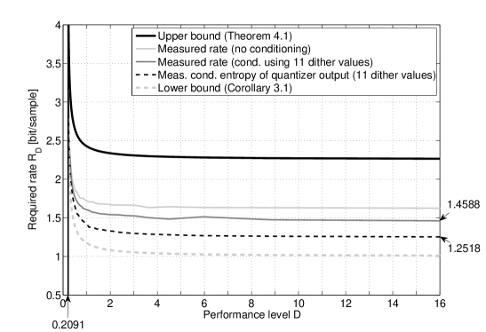
Figure 6: Bounds on the minimal average data rate required to attain a given closed-loop performance level.

Assume that the plant $P$ in Figure 1 is such that

$$y=\dfrac{0.165}{(z-2)(z-0.5789)}(u+d),\quad e=y$$ (43)

and that $(x_{o},d)$ is Gaussian with $d$ being unit-variance white noise. By using the results of Sections III and IV we computed upper and lower bounds on $\mathscr{R}(D)$ for several values of $D>D_{\inf}=0.2091$. We also simulated an actual ECDQ-based linear source coding scheme for each considered value for $D$. To that end, we followed the suggestions at the end of Section V-B and simulated ECDQs where the dither is uniform and perfectly known at both ends of the channels, and where the entropy-coders work conditioned upon a quantized version of the dither. The results are presented in Figure 6. In that figure we plot our upper and lower bounds, and several other curves which report simulation results. All simulation results (referred to as “Measured” in Figure 6) are averages over twenty $10^{4}$-samples-long realizations. In particular, “Measured rate (no conditioning)” corresponds to the average data rate in a case where an empirically-tuned entropy-coder is employed which does not make use of the knowledge of the dither values. Even in this case our upper bound proves to be rather loose. The curve “Measured rate (cond. using 11 dither values)” corresponds to the rate achieved when using and entropy coder that works conditioned upon $11$ uniformly-quantized dither values. As expected our results show that conditioning reduces the incurred average data-rate. (Simulations suggested that using more than $11$ quantized dither values brings only negligible benefits in terms of rate reduction.) The curve “Measured entropy of quantizer output (11 dither values)” corresponds to an empirical estimate of the conditional entropy of the quantizer output $s$, given the quantized dither values.

Our results show that our upper bound is loose. This is consistent with the fact that our upper bound was derived by using worst case considerations. The gap between the measured rate (with conditioning) and our lower bound is about $0.45$ bits per sample, which is smaller than the worst case gap $\frac{1}{2}\log\left(\frac{2\pi e}{12}\right)+\log 2$ nats per sample (about $1.254$ bits per sample). On the other hand the estimated conditional entropy of the quantizer output, given the dither values, is about $0.25$ bits per sample above the lower bound. This implies that, in our simulations, the $0.46$ bit per sample gap is composed by about $0.21$ bits per sample due to the inefficiency of the considered entropy coders, and by about $0.25$ bits per sample due to the fact that the ECDQ generates uniform and not Gaussian noise.

Our results show that, as expected, achieving a closed loop performance arbitrarily close to the best non networked performance $D_{\inf}$ requires arbitrarily high data rates. Interestingly, however, for this example, it suffices to use less that $3$ bits per sample to achieve a performance that is essentially identical to the best non networked performance. It is also interesting to observe that our bounds, and the measured average data-rates, converge rapidly as $D\to\infty$. Thus, whilst achieving an average data-rate arbitrarily close to the minimal rate for stabilization severely compromises performance [11], our results suggest that the performance loss incurred when forcing the average data rate to be low might be modest in some cases.

VII Conclusions

This paper has studied networked control systems subject to average data rate constraints. In particular, we have obtained a characterization of the minimal average data rate that guarantees a prescribed level of performance. Our results have been derived for LTI plants that have one scalar control input, one scalar sensor output, and that are subject to Gaussian disturbances and initial states. No constraints besides causality have been imposed on the considered source coding schemes which yielded a universal lower bound on the minimal average data rate that guarantees a given performance level. Such bound was derived by noting that optimal performance-rate tradeoffs can be described by source coding schemes that behave like a set of LTI filters and a source of additive white noise. Such insight was then used as motivation for building a source coding scheme capable of achieving rates which are less than $\frac{1}{2}\log\left(\frac{2\pi e}{12}\right)+\log 2$ nats per sample away from our derived lower bound, while satisfying the desired performance level constraint. Such coding schemes are based upon entropy dithered quantizers and constitute conceptually simple coding schemes. A numerical example has been include to illustrate our proposal.

Future work should focus on multiple input and multiple output plant models, multichannel architectures, and on ways of reducing the gap between the derived upper and lower bounds on the minimal average data-rate that guarantees a given performance level.

Appendix A Appendix

A-A Three consequences of assuming $D>D_{\inf}$

In this appendix we show that $D>D_{\inf}$ is sufficient for the optimization problems in (5), (13) and (24) to be feasible. We will make extensive use of the definition of $\gamma^{\prime}(D)$ in (24), the related equations in (36) and (37), the conventions regarding the feedback scheme of Figure 2 made on the paragraph preceding Theorem III.2, and the definitions of ECDQs and ECDQ-based linear source coding schemes made in Section IV.

Figure 7: Standard one-degree-of-freedom feedback loop around the plant $P$.

Consider the feedback system of Figure 7, where $P$, $d$ and $x_{o}$ satisfy Assumption II.1, and the controller $K$ is such that $u(k)=\mathscr{K}_{k}(y^{k})$ for some arbitrary mappings $\mathscr{K}_{k}$. Since $P$ is LTI and all the involved random variables are Gaussian, it follows from well-known results [59] that

$$D_{\inf}=\inf_{K\in\mathcal{S}}\sigma_{e}^{2},$$ (44)

where $\mathcal{S}$ is the set of all proper LTI filters which render the the feedback system of Figure 7 internally stable and well-posed. Our assumptions on $P$ guarantee that the above problem is feasible.

The fact that $D>D_{\inf}$ and that the problem of finding $D_{\inf}$ is feasible, implies that for every $\epsilon\in(0,D-D_{\inf})$, there exists $K_{0}\in\mathcal{S}$ such that, in Figure 7, $\sigma^{2}_{e_{0}}\triangleq\left.\sigma_{e}^{2}\right|_{K=K_{0}}\leq D_{\inf}+\epsilon<D$. Consider the feedback scheme of Figure 2 with $F=1$ and $L=L_{0}$, where $L_{0}$ is such that $v=K_{0}\,y$. Since $K_{0}\in\mathcal{S}$, the above choice renders the feedback system of Fig. 2 internally stable and well-posed for any additive noise variance $\sigma_{q^{\prime}}^{2}\in\mathbb{R}^{+}$. This means that the resulting variance of $v^{\prime}$, say $\sigma^{2}_{v0}$, will be finite. It also means that if $q^{\prime}$ in Fig. 2 is zero-mean AWGN with variance $\sigma_{q^{\prime}}$, then the variances of $e^{\prime}$ and of $v^{\prime}$ will increase to $\sigma^{2}_{e_{0}}+\beta_{0}^{(e)}\sigma_{q^{\prime}}$, and $\sigma^{2}_{v_{0}}+\beta^{(v)}_{0}\sigma^{2}_{q^{\prime}}$, respectively, for some finite factors $\beta^{(e)}_{0},\beta^{(v)}_{0}\geq 0$ which depend only upon $K_{0}$. As a consequence, for every $D>D_{\inf}$, there exists $K_{0}\in\mathcal{S}$ such that in Fig. 2 and for the above choice of filters, $\left.\sigma_{e}^{\prime 2}\right|_{(F,L,\sigma_{q^{\prime}}^{2})=(1,L_{0},\sigma^{2}_{q})}<D_{\inf}+\tfrac{2}{3}(D-D_{\inf})$, by picking $\epsilon=(D-D_{\inf})/3$ and $q^{\prime}$ as zero mean AWGN with variance $\sigma^{2}_{q}=\tfrac{1}{3}(D-D_{\inf})/\beta_{0}$. It immediately follows that the above choice of parameters is also such that, in Figure 2,

$$\left.\gamma^{\prime}\right|_{(F,L,\sigma_{q^{\prime}}^{2})=(1,L_{0},\sigma_{q}^{2})}<\frac{3\beta_{0}^{(e)}\beta_{0}^{(v)}\sigma^{2}_{v_{0}}}{D-D_{\inf}}<\infty.$$ (45)

The latter inequality shows that the problem of finding $\gamma^{\prime}(D)$ in (24) is feasible for any $D>D_{\inf}$ (indeed, feasible while yielding all signals in the system jointly Gaussian). Now, from Jensen’s inequality and the concavity of $\log$, it also follows from (45) that the problem of finding $\phi_{u}^{\prime}(D)$ in (13) is feasible for any $D>D_{\inf}$.

We end this section by showing that the problem of finding $\mathscr{R}(D)$ in (5) is also feasible when $D>D_{\inf}$. To that end, it suffices to consider an ECDQ-based linear source coding scheme to link $y$ and $u$ in Figure 1, with parameters $\Delta=\left(12\sigma_{\inf^{\prime}}^{2}\right)^{1/2}$, $F=1$ and $L=L_{\inf}$. Indeed, by exploiting the properties of the latter choice of parameters (see preceding paragraph), our claim follows by proceeding as in the proof of Theorem IV.1 to show that the above defined ECDQ-based linear source coding scheme satisfies Assumption II.2, renders the NCS of Figure 1 AWSS, and achieves $\sigma_{e}^{2}<D$ at a finite average data rate $\mathscr{R}$.

A-B Auxiliary information-theoretic definitions and results

The following definitions and facts are standard and, unless otherwise stated, can be found in [50]. We assume all random variables to have well defined (joint) probability density functions (pdfs). The pdf of $x$ ($x,y$) is denoted $f(x)$ ($f(x,y)$). $f(x|y)$ refers to the conditional pdf of $x$, given $y$. $\mathcal{E}_{x}\left\{\cdot\right\}$ denotes mean with respect to the distribution of $x$.

The differential entropy of $x$ is defined via $h(x)\triangleq-\mathcal{E}_{x}\left\{\log{f(x)}\right\}$. The conditional differential entropy of $x$, given $y$, is defined via $h(x|y)\triangleq-\mathcal{E}_{x,y}\left\{\log{f(x|y)}\right\}$. The mutual information between two random variables $x$ and $y$ is defined via $I(x;y)\triangleq-\mathcal{E}_{x,y}\left\{\log{\left(f(x)f(y)/f(x,y)\right)}\right\}$. The conditional mutual information between $x$ and $y$, given $z$, is defined via $I(x;y|z)\triangleq I(x,z;y)-I(z;y)$. The following are properties of the above quantities:

1. $I(x;y|z)=h(x|z)-h(x|y,z)$.

2. If $f$ is a deterministic function, then $h(x+f(y)|y)=h(x|y)$.

3. If $x$ and $y$ are independent, then $h(x|y)=h(x)$.

4. $h(x_{0},\cdots,x_{n-1})=\sum_{i=0}^{n-1}h(x_{i}|x_{0},\cdots,x_{i-1})$, where $x_{-1}$ can be taken to be a deterministic constant, in which case $h(x_{0}|x_{-1})=h(x_{0})$.

Lemma B.1

Assume that $(x,z)$ are jointly second-order random variables, $x$ is Gaussian, and $z$ is arbitrarily distributed. Then, $I(x;z)\geq(x;z_{G})$, where $z_{G}$ is such that $(x,z_{G})$ are jointly Gaussian and have the same first- and second-order (cross-) moments as $(x,z)$.

Proof:

Immediate from the proof of Lemma 1 in [60]. $\blacksquare$   $\Box\Box\Box$

Figure 8: Generic feedback system.

Lemma B.2

Consider the generic feedback system of Figure 8, where $S_{1}$ is an arbitrary (hence possibly nonlinear and time-varying) causal dynamic system with initial state $x_{1,\,o}$ and disturbance $d_{1}$, such that $\bar{y}(k)=S_{1,k}(x_{1,\,o},d_{1}^{k},\bar{u}^{k-1})$ for some (possibly nonlinear and time-varying) deterministic mapping $S_{1,k}$, and $S_{2}$ is an arbitrary causal dynamic system with disturbance $d_{2}$ and initial state $x_{2,o}$, such that $\bar{u}(k)=S_{2,k}(x_{2,o},d_{2}^{k},\bar{y}^{k})$ for some (possibly nonlinear and time-varying) deterministic mapping $S_{2,k}$. If $(x_{2,o},d_{2})$ are jointly independent of $(x_{1,\,o},d_{1})$, then

$$\sum_{i=0}^{k-1}I(\bar{u}(i);\bar{y}^{i}|\bar{u}^{i-1})=I(x_{1,\,o},d_{1}^{k-1};\bar{u}^{k-1}).$$ (46)

Proof:

Immediate from [61, Theorem 1].  $\blacksquare$   $\Box\Box\Box$

Lemma B.2 corresponds to a stronger version of Theorem 5.1 in [42]. Indeed, the latter result makes use of additional assumptions on system $S_{2}$, does not take side information into account, and only shows that the left hand side of (46) is lower bounded by the corresponding right-hand side.

References

- [1] G. Nair, F. Fagnani, S. Zampieri, and R. Evans, “Feedback control under data rate constraints: An overview,” Proceedings of the IEEE, vol. 95, no. 1, pp. 108 –137, 2007.
- [2] P. Antsaklis and J. Baillieul, “Special issue on technology of networked control systems,” Proceedings of the IEEE, vol. 95, no. 1, pp. 5–8, 2007.
- [3] D. Delchamps, “Stabilizing a linear system with quantized state feedback,” IEEE Transactions on Automatic Control, vol. 35, no. 8, pp. 916–924, August 1990.
- [4] N. Elia and S. Mitter, “Stabilization of linear systems with limited information,” IEEE Transactions on Automatic Control, vol. 46, no. 9, pp. 1384–1400, 2001.
- [5] M. Fu and L. Xie, “The sector bound approach to quantized feedback control,” IEEE Transactions on Automatic Control, vol. 50, no. 11, pp. 1698–1711, November 2005.
- [6] H. Ishii and B. A. Francis, Limited Data Rate in Control Systems with Networks. Springer, 2002.
- [7] W. Wong and R. Brockett, “Systems with finite communication bandwidth constraints - II: Stabilization with limited information feedback,” IEEE Transactions on Automatic Control, vol. 44, no. 5, pp. 1049–1053, May 1999.
- [8] D. Nešić and D. Liberzon, “A unified framework for design and analysis of networked and quantized control systems,” IEEE Transactions on Automatic Control, vol. 54, no. 4, pp. 732–747, April 2009.
- [9] R. Brockett and D. Liberzon, “Quantized feedback stabilization of linear systems,” IEEE Transactions on Automatic Control, vol. 45, no. 7, pp. 1279–1289, June 2000.
- [10] A. Sahai and S. Mitter, “The necessity and sufficiency of anytime capacity for control over a noisy communication link – Part I: Scalar systems,” IEEE Transactions on Information Theory, vol. 52, no. 8, pp. 3369–3395, Aug. 2006.
- [11] G. Nair and R. Evans, “Stabilizability of stochastic linear systems with finite feedback data rates,” SIAM Journal on Control and Optimization, vol. 43, no. 2, pp. 413–436, 2004.
- [12] S. Tatikonda and S. Mitter, “Control under communication constraints,” IEEE Transactions on Automatic Control, vol. 49, no. 7, pp. 1056–1068, July 2004.
- [13] S. Tatikonda, A. Sahai, and S. Mitter, “Stochastic linear control over a communication channel,” IEEE Transactions on Automatic Control, vol. 49, no. 9, pp. 1549–1561, 2004.
- [14] A. Savkin, “Analysis and synthesis of networked control systems: Topological entropy, observability, robustness and optimal control,” Automatica, vol. 42, pp. 51–62, 2006.
- [15] A. Matveev and A. Savkin, Estimation and control over communication networks. Birkhäuser, 2009.
- [16] C. Charalambous and A. Farhadi, “LQG optimality and separation principle for general discrete time partially observed stochastic systems over finite capacity communication channels,” Automatica, vol. 44, no. 12, pp. 3181–3188, 2008.
- [17] N. Martins and M. Dahleh, “Feedback control in the presence of noisy channels: Bode-like fundamental limitations of performance,” IEEE Transactions on Automatic Control, vol. 53, no. 7, pp. 1604–1615, August 2008.
- [18] K. Okano, S. Hara, and H. Ishii, “Characterization of a complementary sensitivity property in feedback control: An information theoretic approach,” Automatica, vol. 45, no. 2, pp. 504–509, 2009.
- [19] H. Shingin and Y. Ohta, “Disturbance rejection with information constraints: Performance limitations of a scalar system for bounded and Gaussian disturbances,” Automatica, vol. 48, pp. 1111–1116, 2012.
- [20] J. Baillieul, “Feedback Designs in Information Based Control,” Stochastic Theory and Control: Proceedings of a Workshop Held in Lawrence, Kansas, 2002.
- [21] S. Tatikonda and S. Mitter, “Control over noisy channels,” IEEE Transactions on Automatic Control, vol. 49, no. 7, pp. 1196–1201, July 2004.
- [22] G. Nair and R. Evans, “Exponential stabilisability of finite-dimensional linear systems with limited data rates,” Automatica, vol. 39, no. 4, pp. 585–593, April 2003.
- [23] F. Fagnani and S. Zampieri, “Stability analysis and synthesis for scalar linear systems with a quantized feedback,” IEEE Transactions on Automatic Control, vol. 48, no. 9, pp. 1569–1584, Sept. 2003.
- [24] K. You and L. Xie, “Minimum data rate for mean square stabilizability of linear systems with Markovian packet losses,” IEEE Transactions on Automatic Control, vol. 56, no. 4, pp. 772–785, 2011.
- [25] P. Minero, L. Coviello, and M. Franceschetti, “Stabilization over markov feedback channels: The general case,” IEEE Transactions on Automatic Control, vol. 58, no. 2, pp. 349–362, February 2013.
- [26] P. Minero, M. Franceschetti, S. Dey, and G. Nair, “Data rate theorem for stabilization over time-varying feedback channels,” IEEE Transactions on Automatic Control, vol. 54, no. 2, pp. 243–255, 2009.
- [27] N. Martins, M. Dahleh, and N. Elia, “Feedback stabilization of uncertain systems in the presence of a direct link,” IEEE Transactions on Automatic Control, vol. 51, no. 3, pp. 438–447, 2006.
- [28] S. Yüksel and T. Basar, “Control over noisy forward and reverse channels,” IEEE Transactions on Automatic Control, vol. 56, no. 5, pp. 1014–1029, 2011.
- [29] D. Neuhoff and R. Gilbert, “Causal source codes,” IEEE Transactions on Information Theory, vol. 28, no. 5, pp. 701–713, 1982.
- [30] T. Linder and R. Zamir, “Causal coding of stationary sources and individual sequences with high resolution,” IEEE Transactions on Information Theory, vol. 52, no. 2, pp. 662–680, 2006.
- [31] M. Derpich and J. Østergaard, “Improved upper bounds to the causal quadratic rate-distortion function for Gaussian stationary sources,” IEEE Transactions on Information Theory, vol. 58, no. 5, pp. 3131–3152, May 2012.
- [32] V. Borkar, S. Mitter, and S. Tatikonda, “Optimal sequential vector quantization of Markov sources,” SIAM Journal on Control and Optimization, vol. 40, no. 1, pp. 135–148, 2001.
- [33] S. Yüksel and T. Linder, “On optimal zero-delay quantization of vector markov sources,” in Proceedings of the 51st IEEE Conference on Decision and Control, Maui, USA, 2012, pp. 6126–6131.
- [34] S. Yüksel and T. Başar, “Minimum rate coding for LTI systems over noiseless channels,” IEEE Transactions on Automatic Control, vol. 51, no. 12, pp. 1878–1887, 2006.
- [35] M. Huang, G. Nair, and R. Evans, “Finite Horizon LQ Optimal Control and Computation with Data Rate Constraints,” in Decision and Control, 2005 and 2005 European Control Conference. CDC-ECC’05. 44th IEEE Conference on, 2006.
- [36] M. Lemmon and R. Sun, “Performance-rate functions for dynamically quantized feedback systems,” in Proceedings of the 45th IEEE Conference on Decision and Control, December 2006.
- [37] M. Fu, “Lack of separation principle for quantized linear quadratic Gaussian control,” IEEE Transactions on Automatic Control, vol. 57, no. 9, pp. 2385–2390, 2012.
- [38] L. Bao, M. Skoglund, and K. Johansson, “Iterative encoder-controller design for feedback control over noisy channels,” IEEE Transactions on Automatic Control, vol. 56, no. 2, pp. 265–278, 2011.
- [39] A. Mahajan and D. Teneketzis, “Optimal Performance of Networked Control Systems with Nonclassical Information Structures,” SIAM Journal on Control and Optimization, vol. 48, no. 3, pp. 1377–1404, 2009.
- [40] J. Massey, “Causality, feedback and directed information,” in Proc. of the International Symposium on Information Theory and its Applications., Hawaii, USA, 1990.
- [41] E. Silva, M. Derpich, and J. Østergaard, “A framework for control system design subject to average data-rate constraints,” IEEE Transactions on Automatic Control, vol. 56, no. 8, pp. 1886–1899, August 2011.
- [42] N. Martins and M. Dahleh, “Fundamental limitations of performance in the presence of finite capacity feedback,” in Proceedings of the American Control Conference, Portland, USA, 2005.
- [43] R. Zamir and M. Feder, “On universal quantization by randomized uniform/lattice quantizers,” IEEE Transactions on Information Theory, vol. 38, no. 2, pp. 428–436, 1992.
- [44] J. Braslavsky, R. Middleton, and J. Freudenberg, “Feedback stabilization over signal-to-noise ratio constrained channels,” IEEE Transactions on Automatic Control, vol. 52, no. 8, pp. 1391–1403, 2007.
- [45] E. Silva, G. Goodwin, and D. Quevedo, “Control system design subject to SNR constraints,” Automatica, vol. 46, no. 2, pp. 428–436, 2010.
- [46] E. Johannesson, “Control and communication with signal-to-noise ratio constraints,” Ph.D. dissertation, Department of Automatic Control, Lund University, Sweden, 2011.
- [47] E. Silva, M. Derpich, and J. Østergaard, “An achievable data-rate region subject to a stationary performance constraint for LTI plants,” IEEE Transactions on Automatic Control, vol. 56, no. 8, pp. 1968–1973, August 2011.
- [48] ——, “On the minimal average data-rate that guarantees a given closed loop performance level,” in Proceedings of the 2nd IFAC Workshop on Distributed Estimation and Control in Networked Systems, Annecy, France, 2010.
- [49] J. Doob, Stochastic Processes. Wiley, 1953.
- [50] T. Cover and J. Thomas, Elements of Information Theory, 2nd ed. John Wiley and Sons, Inc., 2006.
- [51] O. Costa, M. Fragoso, and R. Marques, Discrete Time Markov Jump Linear Systems. Springer, 2005.
- [52] S. Boyd and L. Vandenberghe, Convex Optimization. Cambridge University Press, 2004.
- [53] B. Porat, Digital processing of random signals: theory and methods. Prentice-Hall, Inc., 1994.
- [54] N. Martins, M. Dahleh, and J. Doyle, “Fundamental limitations of disturbance attenuation in the presence of side information,” IEEE Transactions on Automatic Control, vol. 52, no. 1, pp. 56–66, 2007.
- [55] N. Elia, “When Bode meets Shannon: Control oriented feedback communication schemes,” IEEE Transactions on Automatic Control, vol. 49, no. 9, pp. 1477–1488, September 2004.
- [56] B. Francis, A Course on Control Theory. Springer, 1987.
- [57] E. Silva and S. Pulgar, “Control of LTI plants over erasure channels,” Automatica, vol. 47, no. 8, pp. 1729 –1736, August 2011.
- [58] J. Freudenberg, R. Middleton, and J. Braslavsky, “Stabilization with disturbance attenuation over a Gaussian channel,” in Proceedings of the 46th IEEE Conference on Decision and Control, New Orleans, USA, 2007.
- [59] K. Åström, Introduction to Stochastic Control Theory. New York: Academic Press, 1970.
- [60] M. S. Derpich, J. Østergaard, and G. C. Goodwin, “The quadratic Gaussian rate-distortion function for source uncorrelated distortions,” Snowbird, UT, March 2008, pp. 73–82.
- [61] M. Derpich, E. I. Silva, and J. Østergaard, “Fundamental inequalities and identities involving mutual and directed informations in closed-loop systems,” IEEE Transactions on Information Theory, 2013, submitted to IEEE Transactions on Information Theory (available from arXiv).