Atomistic/Continuum Blending
with Ghost Force Correction

Abstract.

We combine the ideas of atomistic/continuum energy blending and ghost force correction to obtain an energy-based atomistic/continuum coupling scheme which has, for a range of benchmark problems, the same convergence rates as optimal force-based coupling schemes.

We present the construction of this new scheme, numerical results exploring its accuracy in comparison with established schemes, as well as a rigorous error analysis for an instructive special case.

1. Introduction

Atomistic/continuum coupling schemes are a popular class of multi-scale methods for concurrent coupling between atomistic and continuum mechanics in the simulation of crystalline solids. An ongoing effort to develop a rigorous numerical analysis, summarised in [12], has led to a distillation of many key ideas in the field, and a number of improvements.

It remains an open problem to construct a general and practical QNL-type a/c coupling scheme along the lines of [23, 5, 21]. The present paper develops an a/c coupling approach combining two popular practical schemes, ghost force correction [22] and blending [25], as well as its rigorous analysis.

In the ghost force correction method of Shenoy et al [22] the spurious interface forces caused by a/c coupling (usually termed ghost forces) are removed by adding a suitable dead load correction, which can be computed either from a previous step in a quasi-static process or through a self-consistent iteration. In the latter case, this process was shown to be formally equivalent to the force-based quasicontinuum (QCF) scheme [3]. Difficult open problems remain in the analysis of the QCF method; see [11, 4, 10, 14] for recent advances, however in practice the scheme seems to be optimal (in terms of the error committed by the coupling mechanism). The main drawback is that the QCF forces are non-conservative, i.e., there is no associated energy functional.

An alternative scheme to reduce the effect of ghost forces is the blending method of Xiao and Belytschko [25]. Instead of a sharp a/c interface, the atomistic and continuum models are blended smoothly. This does not remove, but reduce the error due to ghost forces [24, 9]. The blending variant that we will consider is the BQCE scheme, formulated in [24, 13] and analysed in [24, 9]. These analyses demonstrate that altough the error due to ghost forces is reduced, it still remains the dominant error contribution, i.e., the bottleneck. Moreover, if one were to generalize the BQCE scheme to multi-lattices, then the reduced symmetries imply that the scheme would not be convergent (in the sense of [9]).

In the present paper, we show how a variant of the ghost force correction idea can be used to improve on the BQCE scheme and to result in an a/c coupling that we denote blended ghost force correction (BGFC), which is quasi-optimal within the context of the framework developed in [9]. Importantly, within the context in which we present this scheme, our formulation does not yield the force-based BQCF scheme [11, 9, 8] but is energy-based. As a matter of fact, it is most instructive to construct the scheme not from the point of view of ghost-force correction, but through a modification of the site energies.

The remainder of the article is structured as follows. In § 2 we formulate the BGFC scheme for point defects. In § 3 we extend the benchmark tests from [13, 8, 21] to the new scheme. In § 4 we briefly describe extensions to higher-order finite element, dislocations and multi-lattices. Finally, in § 5 we present a rigorous error analysis for the simple-lattice point defect case.

2. The BGFC Scheme

For the sake of simplicity of presentation we first present the BGFC scheme in an infinite lattice setting and for point defects. This also allows us to focus on the benchmark problems discussed in [8, 13, 21] which are the main motivation for the introduction of our new scheme. We present extensions to other problems in § 4.

2.1. Atomistic model

Consider a homogeneous reference lattice $\Lambda^{\rm hom}:={\sf A}\mathbb{Z}^{d}$, $d\in\{2,3\}$, ${\sf A}\in\mathbb{R}^{d\times d}$, non-singular. Let $\Lambda\subset\mathbb{R}^{d}$ be the reference configuration, satisfying $\Lambda\setminus B_{R^{\rm def}}=\Lambda^{\rm hom}\setminus B_{R^{\rm def}}$ and $\#(\Lambda\cap B_{R^{\rm def}})<\infty$, for some radius $R^{\rm def}>0$. Here, and throughout, $B_{R}:=\{x\in\mathbb{R}^{d}\,|\,|x|\leq R\}$.

The mismatch between $\Lambda$ and $\Lambda^{\rm hom}$ in $B_{R^{\rm def}}$ represents a possible defect. For example, $\Lambda=\Lambda^{\rm hom}$ for an impurity, $\Lambda\subset\Lambda^{\rm hom}$ for a vacancy and $\Lambda\supset\Lambda^{\rm hom}$ for an interstitial.

For $a\in\Lambda$, let $\mathcal{N}_{a}\subset\Lambda\setminus\{a\}$ be a set of “nearest-neighbour” directions satisfying ${\rm span}(\mathcal{N}_{a})=\mathbb{R}^{d}$ and $\sup_{a\in\Lambda}\#\mathcal{N}_{a}<\infty$.

A deformed configuration is a map $y:\Lambda\to\mathbb{R}^{d}$. If it is clear from the context what we mean, then we denote $r_{ab}:=|y(a)-y(b)|$ for $a,b\in\Lambda$. We denote the identity map by $x$.

For each $a\in\Lambda$ let $\Phi_{a}(y)$ denote the site energy associated with the lattice site $a\in\Lambda$. For example, in the EAM model [1],

$$\Phi_{a}(y):=\sum_{b\in\Lambda\setminus\{a\}}\phi(r_{ab})+G\Big{(}{\textstyle\sum_{b\in\Lambda\setminus\{a\}}}\rho(r_{ab})\Big{)},$$ (2.1)

for a pair potential $\phi$, an electron density function $\rho$ and an embedding function $G$. We assume that the potentials have a finite interaction range, that is, there exists $r_{\rm cut}>0$ such that $\partial_{y(b)}^{j}\Phi_{a}(y)=0$ for all $j\geq 1$, whenever $r_{ab}>r_{\rm cut}$, and that they are homogeneous outside the defect region $B_{R^{\rm def}}$. The latter assumption is discussed in detail in § 2.2.

To describe, e.g., impurity defects, we allow $\phi,G,\rho$ to be species-dependent, i.e., $\phi=\phi_{ab},G=G_{a},\psi=\psi_{ab}$.

Under suitable conditions on the site potentials $\Phi_{a},a\in\Lambda$ (most crucially, regularity and homogeneity outside the defect; cf. § 2.2), it is shown in [7] that the energy-difference functional

$$\mathscr{E}^{\rm a}(u):=\sum_{a\in\Lambda}\Phi^{\prime}_{a}(u),\qquad\text{where }\Phi^{\prime}_{a}(u):=\Phi_{a}(x+u)-\Phi_{a}(x),$$ (2.2)

is well-defined for all relative displacements $u\in\mathscr{U}$, where $\mathscr{U}$ is given by

$$\mathscr{U} :=\big{\{}v:\Lambda\to\mathbb{R}^{d}\,\big{|}\,|v|_{\mathscr{U}}<+\infty\big{\}},\quad\text{where}$$

$$|v|_{\mathscr{U}} :=\Big{(}\sum_{a\in\Lambda}\sum_{b\in\mathcal{N}_{a}}|v(b)-v(a)|^{2}\Big{)}^{1/2}.$$

The atomistic problem is to compute

$$u^{\rm a}\in\arg\min\big{\{}\mathscr{E}^{\rm a}(v)\,\big{|}\,v\in\mathscr{U}\big{\}}.$$ (2.3)

This problem is analysed in considerable detail in [7].

2.2. Homogeneous crystals

We briefly discuss homogeneity of site potentials, a concept which is important for the introduction of the BGFC scheme, and also plays a crucial role in the definition of the atomistic model (2.3).

Homogeneity of the site potential outside the defect core entails simply that only one atomic species occurs. For finite-range interactions, this can be formalised by requiring that, for $|a|,|b|$ sufficiently large, $\Phi_{a}(y)=\Phi_{b}(z)$ where $z(\ell)=y(\ell+a-b)$ within the interaction range of $b$, and suitably extended outside.

For the case $\Lambda=\Lambda^{\rm hom}$ we say that the site potentials are globally homogeneous if $\Phi_{a}(y)=\Phi_{b}(z)$ for all $a,b\in\Lambda^{\rm hom}$. In this case, it is easy to see (summation by parts, or point-symmetry of the lattice) that

$$\sum_{a\in\Lambda^{\rm hom}}\big{\langle}\delta\Phi_{a}(x),u\big{\rangle}=0\qquad\forall u:\Lambda^{\rm hom}\to\mathbb{R}^{d},{\rm supp}(u)\text{~{}compact}.$$

For general $\Lambda$, suppose that the site potentials are homogeneous outside $B_{R^{\rm def}}$, with finite interaction range. Let $\Phi_{a}^{\rm hom},a\in\Lambda^{\rm hom}$ be a globally homogeneous site potential so that $\langle\delta\Phi_{a}(x),u\rangle=\langle\delta\Phi_{a}^{\rm hom},u\rangle$ for all $a\in\Lambda,|a|>R^{\rm def}+r_{\rm cut}$ and for all $u:\Lambda\cup\Lambda^{\rm hom}\to\mathbb{R}^{d}$ with compact support. Further, for $u:\Lambda\to\mathbb{R}^{d}$ let $Eu$ denote an arbitrary extension to $\Lambda^{\rm hom}$ (e.g., $Eu(\ell)=0$ for $\ell\in\Lambda^{\rm hom}\setminus\Lambda$), and let $\Lambda_{\rm def}:=\Lambda\cap B_{R^{\rm def}+r_{\rm cut}}$, then

$$\mathscr{E}^{\rm a}(u) =\sum_{a\in\Lambda}\Phi_{a}^{\prime}(u)-\sum_{a\in\Lambda^{\rm hom}}\langle\delta\Phi_{a}^{\rm hom}(x),Eu\rangle$$

$$=\sum_{a\in\Lambda}\Phi_{a}^{\prime\prime}(u)+\langle L^{\rm ren},Eu\rangle,$$ (2.4)

where

$$\Phi_{a}^{\prime\prime}(u) :=\Phi_{a}(x+u)-\Phi_{a}(x)-\langle\delta\Phi_{a}(x),Eu\rangle,$$ (2.5)

$$\langle L^{\rm ren},u\rangle :=\sum_{a\in\Lambda_{\rm def}}\langle\delta\Phi_{a}(x),u\rangle-\sum_{a\in\Lambda^{\rm hom}_{\rm def}}\langle\delta\Phi_{a}^{\rm hom}(x),Eu\rangle.$$ (2.6)

The “renormalisation” (2.4) of $\mathscr{E}^{\rm a}$ is the basis for proving that $\mathscr{E}^{\rm a}$ is well-defined on the energy space $\mathscr{U}$ [7].

2.3. Continuum model

Suppose that the site potentials are homogeneous outside the defect core and let $\Phi_{a}^{\rm hom}$ be the associated globally homogeneous site potentials for the homogeneous lattice; cf. § 2.2.

To formulate atomistic to continuum coupling schemes we require a continuum model compatible with (2.2) defined through a strain energy function $W:\mathbb{R}^{d\times d}\to\mathbb{R}$. A typical choice in the multi-scale context is the Cauchy–Born model, which is defined via

$$W({\sf F}):=\det{\sf A}^{-1}\Phi^{\rm hom}_{0}({\sf F}x),$$

which represents the energy per unit volume in the homogeneous crystal ${\sf F}\Lambda^{\rm hom}={\sf F}{\sf A}\mathbb{Z}^{d}$. The associated strain energy difference is denoted by $W^{\prime}({\sf G}):=W({\sf I}+{\sf G})-W({\sf I})$.

2.4. Standard blending scheme

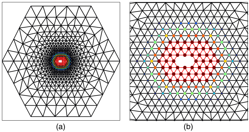
Figure 1. Computational domain, finite element grid and atomistic region as used in the construction of the BQCE and BGFC schemes. The size and color of the spheres in (b) indicate the value of the blending function (large/red stands for $\beta=0$).

To formulate the blended quasicontinuum (BQCE) scheme as introduced in [24, 13] and analysed in [9] we begin by defining a regular simplicial finite element grid $\mathcal{T}_{h}$ with nodes $\mathcal{X}_{h}$, with the minimal requirement that $\mathcal{X}_{h}\cap B_{R^{\rm def}}=\Lambda\cap B_{R^{\rm def}}$ (that is, the defect core is resolved exactly). Let ${\rm DOF}:=\#\mathcal{X}_{h}$. Let ${\Omega_{h}}:=\bigcup\mathcal{T}_{h}\supset B_{R^{\rm c}}$, with $R^{\rm c}\geq R^{\rm def}$ be the resulting computational domain and let the space of coarse-grained admissible displacements be given by

$$\mathscr{U}_{h}:=\big{\{}v_{h}\in C(\mathbb{R}^{d};\mathbb{R}^{d})\,\big{|}\,v_{h}\text{ is p.w. affine w.r.t. }\mathcal{T}_{h},\text{ and }v_{h}|_{\mathbb{R}^{d}\setminus{\Omega_{h}}}=0\big{\}}.$$

Let $Q_{h}$ denote the P0 midpoint interpolation operator, so that $\int_{{\Omega_{h}}}Q_{h}f$ is the midpoint rule approximation to $\int_{{\Omega_{h}}}f$.

Further, let $\beta\in C^{2,1}(\mathbb{R}^{d})$ with $\beta=0$ in $B_{R^{\rm a}}$ with $R^{\rm def}\leq R^{\rm a}<R^{\rm c}$ and $\beta=1$ in $\mathbb{R}^{d}\setminus{\Omega_{h}}$, then we define the BQCE energy functional

$$\mathscr{E}^{\rm b}(u_{h}):=\sum_{a\in\Lambda\cap{\Omega_{h}}}(1-\beta(a))\Phi_{a}^{\prime}(u)+\int_{{\Omega_{h}}}Q_{h}\big{[}\beta W^{\prime}(\nabla u_{h})\big{]}.$$

The BQCE problem is to compute

$$u^{\rm b}_{h}\in\arg\min\big{\{}\mathscr{E}^{\rm b}(v_{h})\,\big{|}\,v_{h}\in\mathscr{U}_{h}\big{\}}.$$ (2.7)

2.5. Review of error estimates

We present a formal review of error estimates for the BQCE scheme established in [13, 9]. This discussion will motivate our construction of the BGFC scheme in the next section.

Under a range of technical assumptions on $\mathcal{T}_{h}$ and $\beta$ it is shown in [9] that, if $u^{\rm a}$ is a strongly stable (positivity of the hessian) solution to (2.3), and $(\beta,\mathcal{T}_{h})$ are “sufficiently well-adapted to $u^{\rm a}$”, then there exists a solution $u^{\rm b}_{h}$ to (2.7) such that

$$\|\nabla u^{\rm b}_{h}-\nabla\overline{u^{\rm a}}\|_{L^{2}}\leq C_{1}\|\nabla^{2}\beta\|_{L^{2}}+C_{2}\Big{(}\|\beta h\nabla^{2}\widetilde{u^{\rm a}}\|_{L^{2}({\Omega_{h}})}+\|\nabla\widetilde{u^{\rm a}}\|_{L^{2}(\mathbb{R}^{d}\setminus B_{R^{\rm c}/2})}\Big{)}+\dots,$$ (2.8)

where “$\dots$” denotes formally higher order terms, $\overline{u^{\rm a}}$ denotes a P1 interpolant on the atomistic grid $\Lambda$ and $\widetilde{u^{\rm a}}$ a $C^{2,1}$-conforming interpolant on the atomistic grid $\Lambda$ (intuitively, $\nabla^{j}\widetilde{u^{\rm a}}$, $j\geq 2$, measure the local regularity of $u^{\rm a}$; see § 5 and [9] for more details). The constants depend on (derivatives of) $\Phi_{a},a\in\Lambda,$ in a way that we will discuss in more detail below.

The term $\|\beta h\nabla^{2}\widetilde{u^{\rm a}}\|_{L^{2}({\Omega_{h}})}$ measures the finite element approximation error while the term $\|\nabla\widetilde{u^{\rm a}}\|_{L^{2}(\mathbb{R}^{d}\setminus B_{R^{\rm c}/2})}$ measures the error committed by truncating to a finite computational domain. Exploiting the generic decay rates [7]

$$|\nabla^{j}\widetilde{u^{\rm a}}(x)|\lesssim|x|^{1-d-j}\quad\text{as $j\to\infty$},$$ (2.9)

these terms can be balanced by ensuring that $R^{\rm c}\approx(R^{\rm a})^{2}$ and the mesh is coarsened according to $h(x)\approx(|x|/R^{\rm a})^{3/2}$ (see [19]), which yields

$$\|\beta h\nabla^{2}\widetilde{u^{\rm a}}\|_{L^{2}({\Omega_{h}})}+\|\nabla\widetilde{u^{\rm a}}\|_{L^{2}(\mathbb{R}^{d}\setminus B_{R^{\rm c}/2})}\lesssim({\rm DOF})^{-1/2-1/d}.$$

By contrast, the term $\|\nabla^{2}\beta\|_{L^{2}}$ is due to the (smeared) ghost forces, and even an optimal choice of $\beta$ (balanced against the atomistic region radius $R^{\rm a}$) yields only

$$\|\nabla^{2}\beta\|_{L^{2}}\approx({\rm DOF})^{1/2-2/d}.$$ (2.10)

To see this, we note that, a quasi-optimal choice is $\beta(x)=B(r)$, where $B$ is a radial spline with $B(r)=0$ for $r\leq R^{\rm a}$ and $B(r)=1$ for $r\geq R^{\rm b}\in(R^{\rm a},R^{\rm c})$ (see [24, 13] for in-depth discussions). A straightforward computation (assuming $R^{\rm b}\lesssim R^{\rm a}$; the case $R^{\rm b}\gg R^{\rm a}$ is similar) then shows that $\|\nabla^{2}\beta\|_{L^{2}}^{2}\approx(R^{\rm b})^{d-1}(R^{\rm b}-R^{\rm a})^{-3}+(R^{\rm b}-R^{\rm a})^{d-4}$, which is optimised subject to fixing the total number of degrees of freedom if $R^{\rm b}-R^{\rm a}\approx R^{\rm a}$. This yields precisely (2.10).

In summary, for this simple model problem, the BQCE scheme’s rate of convergence,

$$\|\nabla u^{\rm b}_{h}-\nabla\overline{u^{\rm a}}\|_{L^{2}}\lesssim({\rm DOF})^{1/2-2/d},$$

is the same in 2D and worse in 3D than a straightforward truncation scheme, in which the atomistic model is minimised over a finite computational domain (see [7]). Analogous results hold also for dislocations.

2.6. The BGFC scheme

The motivation for the BGFC scheme is to optimise the coefficient $C_{1}$ in (2.8). An investigation of the analysis in § 6.1 and § 6.2 in [9] reveals that a simple upper bound is

$$C_{1}\lesssim\sup_{a\in\Lambda\cap{\rm supp}(\beta)}\sup_{b\in\Lambda\setminus\{a\}}\Big{|}\frac{\partial\Phi_{a}(y)}{\partial y(b)}|_{y=x+u}\Big{|}.$$

(As a matter of fact, this form of $C_{1}$ requires a minor modification of the remaining error estimates [9]; however, we use it only for motivation.)

The idea is to “renormalise” the interatomic potential so that $\delta\Phi_{a}(x)=0$ for $|a|$ sufficiently large, which would then ensure that $|\partial_{y(b)}\Phi_{a}(x+u)|\lesssim|u(b)-u(a)|$ and hence would yield additional decay of the constant $C_{1}$ as the atomistic region increases.

Recalling the discussion in § 2.2 we note that $\delta\Phi_{a}^{\prime\prime}(x)=0$ for all $a\in\Lambda$. Thus, if we apply the blending procedure to the renormalised atomistic energy (2.4) then we would obtain a new constant $C_{1}^{\prime\prime}$ with

$$C_{1}^{\prime\prime} \lesssim\sup_{a\in\Lambda\cap{\rm supp}(\nabla\beta)}\sup_{\begin{subarray}{c}b\in\Lambda\setminus\{a\}\\ r_{ab}\leq r_{\rm cut}\end{subarray}}\big{|}\partial_{y(b)}\Phi_{a}^{\prime\prime}(x+u)\big{|}$$

$$=\sup_{a\in\Lambda\cap{\rm supp}(\nabla\beta)}\sup_{\begin{subarray}{c}b\in\Lambda\setminus\{a\}\\ r_{ab}\leq r_{\rm cut}\end{subarray}}\big{|}\partial_{y(b)}\Phi_{a}(x+u)-\partial_{y(b)}\Phi_{a}(x)\big{|}$$

$$\lesssim C_{2}\big{\|}\nabla\overline{u^{\rm a}}\big{\|}_{L^{\infty}(\mathbb{R}^{d}\setminus B_{R^{\rm a}-2r_{\rm cut}})}\lesssim(R^{\rm a})^{-d}.$$

where the second to last inequality is true for sufficiently large $R^{\rm a}$ and the last inequality follows from the decay estimate given in [7, Thm. 3.1]. We therefore obtain

$$C_{1}^{\prime\prime}\|\nabla^{2}\beta\|_{L^{2}}\lesssim({\rm DOF})^{-1/2-2/d},$$ (2.11)

which not only balances the best approximation error but is even dominated by it.

To summarize, the BGFC energy (difference) functional reads

$$\mathscr{E}^{\rm bg}(u_{h}):=\sum_{a\in\Lambda\cap{\Omega_{h}}}(1-\beta(a))\Phi_{a}^{\prime\prime}(u_{h})+\int_{{\Omega_{h}}}Q_{h}\big{[}\beta W^{\prime\prime}(\nabla u_{h})\big{]}+\langle L^{\rm ren},u_{h}\rangle,$$ (2.12)

where $\Phi_{a}^{\prime\prime}$ is defined in (2.5), $L^{\rm ren}$ in (2.6) and $W^{\prime\prime}({\sf F}):=W({\sf I}+{\sf F})-W({\sf I})-\partial W({\sf I}):{\sf F}$. The associated variational problem is

$$u^{\rm bg}_{h}\in\arg\min\big{\{}\mathscr{E}^{\rm bg}(v_{h})\,\big{|}\,v_{h}\in\mathscr{U}_{h}\big{\}}.$$ (2.13)

We can further optimise the BGFC scheme as follows. If $R^{\rm b}/R^{\rm a}\sim c$ as $R^{\rm a}\to\infty$, then the coupling error of the BGFC scheme scales like $(R^{\rm a})^{-d/2-2}$, and is therefore dominated by the best approximation error, which scales like $(R^{\rm a})^{-d/2-1}$. To reduce computational cost (by a constant factor), we can balance these two terms. Making the ansatz $R^{\rm b}-R^{\rm a}\sim(R^{\rm a})^{t}$, for $t\in(0,1)$, and noting that we can always construct $\beta$ such that $|\nabla^{2}\beta|\lesssim(R^{\rm a})^{-t}$, we obtain that

$$C_{1}^{\prime\prime}\|\nabla^{2}\beta\|_{L^{2}}\lesssim(R^{\rm a})^{-d/2-3/2-1/2}.$$

This is balanced with the best approximation rate, $(R^{\rm a})^{-d/2-1}$, if $t=1/3$.

We therefore conclude that, if $R^{\rm b}-R^{\rm a}\approx(R^{\rm a})^{t}$ for some $t\geq 1/3$, then we expect the BGFC scheme to obey the error estimate

$$\|\nabla u^{\rm bg}_{h}-\nabla\overline{u^{\rm a}}\|_{L^{2}}\lesssim(R^{\rm a})^{-d/2-1}\approx({\rm DOF})^{-1/2-1/d}.$$

We shall make this rigorous for a slightly simplified formulation in § 5, where we will also prove an energy error estimate.

2.7. Connection to ghost-force correction and generalisation

Consider, for simplicity, the case when $\Phi^{\rm hom}_{a}\equiv\Phi_{a}$, i.e., the crystal is homogeneous. In this case, $L^{\rm ren}\equiv 0$ as well. Moreover, we can rewrite the BGFC scheme as follows:

$$\mathscr{E}^{\rm bg}(u_{h}) =\mathscr{E}^{\rm b}(u_{h})-\sum_{a\in\Lambda}(1-\beta(a))\langle\delta\Phi_{a}(0),u_{h}\rangle-\int_{\mathbb{R}^{d}}Q_{h}\big{[}\beta\partial W(0):\nabla u_{h}\big{]}\,{\rm d}x$$

$$=\mathscr{E}^{\rm b}(u_{h})-\langle\delta\mathscr{E}^{\rm b}(0),u_{h}\rangle$$

$$=\mathscr{E}^{\rm b}(u_{h})-\langle\delta\mathscr{E}^{\rm b}(0)-\mathcal{F}^{\rm bqcf}(0),u_{h}\rangle,$$ (2.14)

where $\mathcal{F}^{\rm bqcf}$ is the BQCF operator defined in [8], and $\mathcal{F}^{\rm bqcf}(0)=0$ (this non-conservative a/c coupling has no ghost forces). Thus, we see that the renormalisation step $\Phi^{\prime}_{a}\leadsto\Phi_{a}^{\prime\prime}$ (cf. (2.2) and (2.5)) is equivalent to the dead load ghost-force correction scheme of Shenoy at al [22], applied for a blended coupling formulation and in the reference configuration.

This immediately suggests the following generalisation of the BGFC scheme:

$$\mathscr{E}^{\rm bg}(u_{h}):=\mathscr{E}^{\rm b}(u_{h})-\big{\langle}\delta\mathscr{E}^{\rm b}(\hat{u}_{h})-\mathcal{F}^{\rm bqcf}(\hat{u}_{h}),u_{h}-\hat{u}_{h}\big{\rangle},$$ (2.15)

where $\hat{u}_{h}$ is a suitable reference configuration, or “predictor”, that can be cheaply obtained.

We will explore this alternative point of view in future work, in particular with an eye to applications involving cracks and edge dislocations.

3. Numerical Tests

3.1. Model problems

Our prototype implementation of BGFC is for the 2D triangular lattice ${\sf A}\mathbb{Z}^{2}$ defined by

$${\sf A}=\begin{pmatrix}1&\cos(\pi/3)\\ 0&\sin(\pi/3)\end{pmatrix}.$$

To generate a defect, we remove $k$ atoms

$$\left\{\begin{array}[]{rl}\Lambda^{\rm def}_{k}:=\big{\{}-(k/2+1)e_{1},\dots,k/2e_{1}\big{\}},&\text{ if $k$ is even, }\\[2.84526pt] \Lambda^{\rm def}_{k}:=\big{\{}-(k-1)/2e_{1},\dots,(k-1)/2e_{1}\big{\}},&\text{ if $k$ is odd,}\end{array}\right.$$

to obtain $\Lambda:={\sf A}\mathbb{Z}^{2}\setminus\Lambda^{\rm def}_{k}$. For small $k$, the defect acts like a point defect, while for large $k$ it acts like a small crack embedded in the crystal. In our experiments we shall consider $k=2$ (di-vacancy) and $k=11$ (microcrack), following [13, 8, 21].

The site energy is given by an EAM (toy-)model (3.1) [1], for which $\Phi_{\ell}$ is of the form

$$\Phi_{\ell}(y) =\sum_{\rho\in\mathcal{R}(\ell)}\phi\big{(}|D_{\rho}y(\ell)|\big{)}+F\Big{(}{\textstyle\sum_{\rho\in\mathcal{R}(\ell)}}\psi\big{(}|D_{\rho}y(\ell)|\big{)}\Big{)},$$ (3.1)

with $$\phi(r)=[e^{-2a(r-1)}-2e^{-a(r-1)}],\quad\psi(r)=e^{-br},$$

$$F(\tilde{\rho})=c\big{[}(\tilde{\rho}-\tilde{\rho}_{0})^{2}+(\tilde{\rho}-\tilde{\rho}_{0})^{4}\big{]},$$

with parameters $a=4.4,b=3,c=5,\tilde{\rho}_{0}=6e^{-b}$. The interaction range is $\mathcal{R}(\ell)=\Lambda\cap B_{2}(\ell)$, i.e., next nearest neighbors in hopping distance.

To construct the BQCE and BGFC schemes, we choose an elongated hexagonal domain $\Omega^{\rm a}$ containing $K$ layers of atoms surrounding the vacancy sites and the full computational domain $\Omega_{h}$ to be an elongated hexagon containing $R^{\rm c}$ layers of atoms surrounding the vacancy sites. The domain parameters are chosen so that $R^{\rm c}=\lceil{\textstyle\frac{1}{2}}(R^{\rm a})^{2}\rceil$. The finite element mesh is graded so that the mesh size function $h(x)={\rm diam}(T)$ for $T\in\mathscr{T}$ satisfies $h(x)\approx(|x|/R^{\rm a})^{3/2}$. These choices balance the coupling error at the interface, the finite element interpolation error and the far-field truncation error [7, Sec.5.2]. Recall moreover that ${\rm DOF}:=\#\mathcal{X}_{h}$.

The blending function is obtained in a preprocessing step by approximately minimising $\|\nabla^{2}\beta\|_{L^{2}}$, as described in detail in [13].

We implement the equivalent ghost force removal formulation (2.14) instead of the “renormalisation formulation” (2.12).

3.1.1. Di-vacancy

In the di-vacancy test two neighboring sites are removed, i.e., $k=2$. We apply $3\%$ isotropic stretch and $3\%$ shear loading, by setting

$${\sf B}:=\begin{pmatrix}1+s&\gamma_{\rm II}\\ 0&1+s\end{pmatrix}\cdot{\sf F}_{0}.$$

where ${\sf F}_{0}\propto I$ minimizes $W$, $s=\gamma_{\rm II}=0.03$.

3.1.2. Microcrack

In the microcrack experiment, we remove a longer segment of atoms, $\Lambda^{\rm def}_{11}=\{-5e_{1},\dots,5e_{1}\}$ from the computational domain. The body is then loaded in mixed mode ${\rm I}$ & ${\rm II}$, by setting,

$${\sf B}:=\begin{pmatrix}1&\gamma_{\rm II}\\ 0&1+\gamma_{\rm I}\end{pmatrix}\cdot{\sf F}_{0}.$$

where ${\sf F}_{0}\propto I$ minimizes $W$, and $\gamma_{\rm I}=\gamma_{\rm II}=0.03$ ($3\%$ shear and $3\%$ tensile stretch).

3.2. Methods

We shall test BGFC method with blending widths $K:=R^{\rm b}-R^{\rm a}=\lceil(R^{\rm a})^{1/3}\rceil$ and with $K=R^{\rm b}-R^{\rm a}=R^{\rm a}$ (here, the blending width denotes the number of hexagonal atomic layers in the blending region). The BGFC scheme is compared against the 3 competitors previously considered in [13, 8, 21]:

• B-QCE: blended quasicontinuum method, implementation based on [13], with most details described in § 2.4.

• GRAC: sharp-interface consistent energy-based a/c coupling [21].

• B-QCF: blended force-based a/c coupling, as described in [8]. Energies of B-QCF are computed using B-QCE (i.e., the B-QCE energy is evaluated at the B-QCF solution).

3.3. Results

We present two experiments, a di-vacancy ($k=2$) and a microcrack ($k=11$). For each test, we choose an increasing sequence of atomistic region sizes $R^{\rm a}$, followed by the quasi-optimal choices of $R^{\rm b},\Omega_{h},\beta$ as described above.

For both experiments we plot the absolute errors against the number of degrees of freedom (DOF), which is proportional to computational cost, in the $H^{1}$-seminorm, the $W^{1,\infty}$-seminorm and in the (relative) energy.

The results are shown in Figures 2, 3 and 4 for the di-vacancy problem and in Figures 5, 6 and 7 for the microcrack problem.

In the first experiment, we are able to clearly observe the predicted asymptotic behaviour of the a/c coupling schemes, while in the second experiment we observe a significant pre-asymptotic regime where the analytic predictions become relevant only at fairly high resolutions.

In all error graphs we clearly observe the optimal convergence rate of BGFC , together with other consistent methods GRAC and BQCF, while BQCE has a sub-optimal rate.

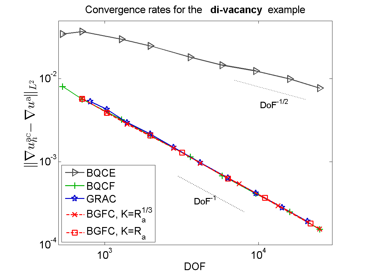
Figure 2. Convergence rates in the energy-norm (the $H^{1}$-seminorm) for the di-vacancy benchmark problem described in Section § 3.1.1 .

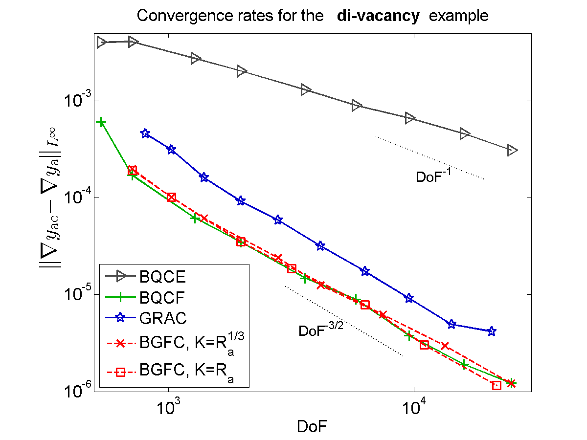
Figure 3. Convergence rates in the $W^{1,\infty}$-seminorm for the di-vacancy benchmark problem described in Section § 3.1.1 .

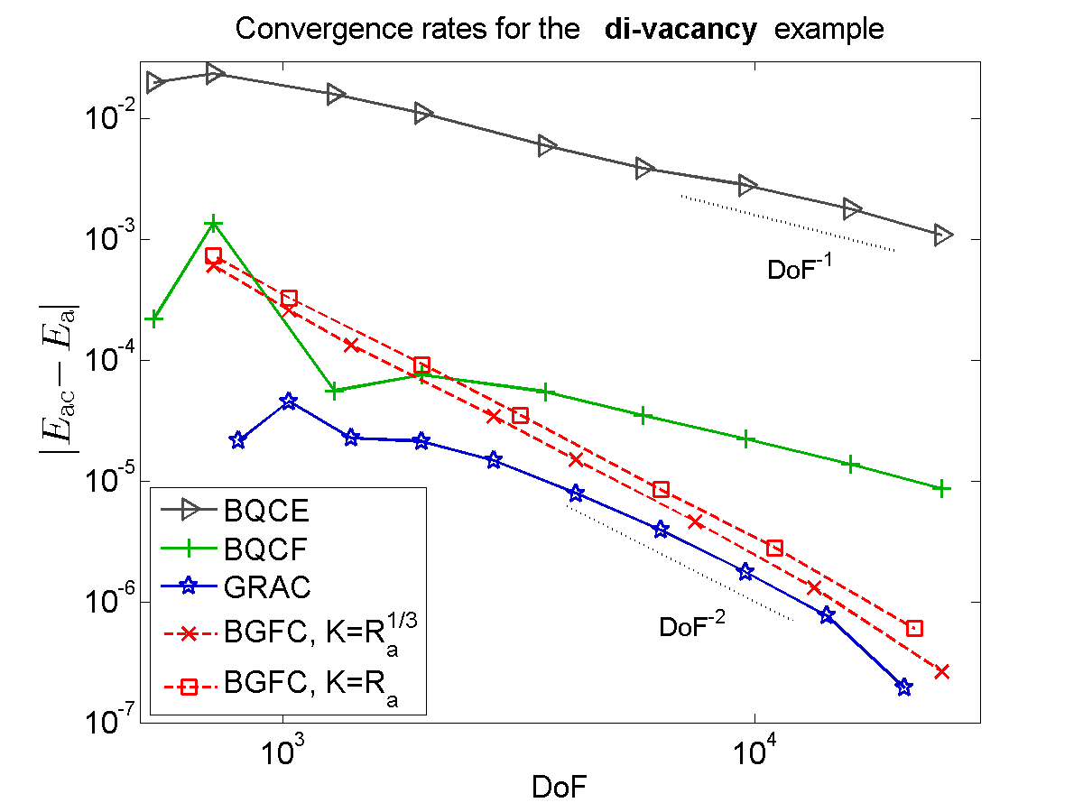
Figure 4. Convergence rates in the relative energy for the di-vacancy benchmark problem described in Section § 3.1.1 .

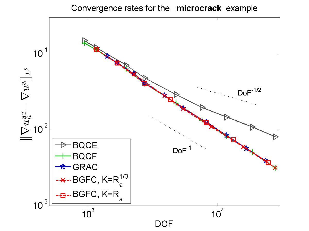
Figure 5. Convergence rates in the energy-norm (the $H^{1}$-seminorm) for the microcrack benchmark problem with $\Lambda^{\rm def}_{11}$ described in Section § 3.1.2 .

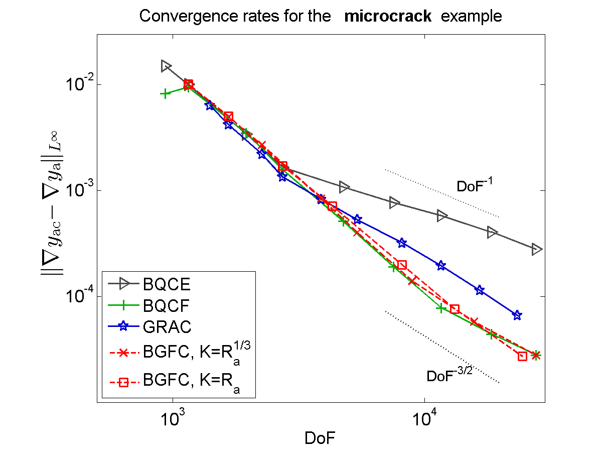
Figure 6. Convergence rates in the $W^{1,\infty}$-seminorm for the microcrack benchmark problem with $\Lambda^{\rm def}_{11}$ described in Section § 3.1.2 .

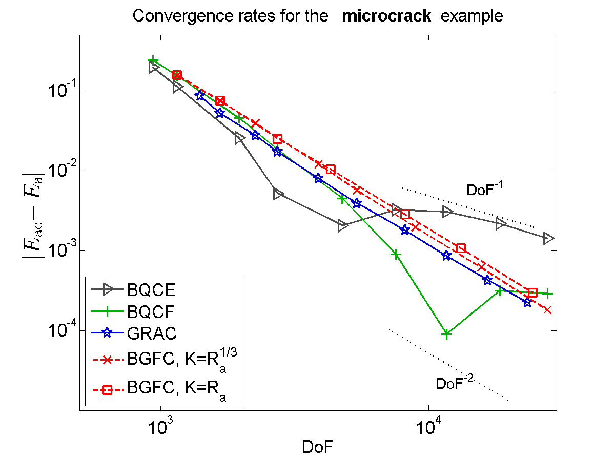
Figure 7. Convergence rates in the relative energy for the microcrack benchmark problem with $\Lambda^{\rm def}_{11}$ described in Section § 3.1.2 .

4. Extensions

It is possible to extend the formulation of the BGFC scheme to a much wider range of problems, including e.g. multiple defect regions, problems with surfaces (e.g., nano-indentation, crack propagation), complex crystals, or higher order finite elements. We now present a range of such generalisations, arguing only formally to motivate a more complete and rigorous treatment in future work.

4.1. Higher-order finite elements

We have seen in § 2.6 that in the BGFC scheme applied to point defects, the approximation error dominates the blending (coupling) error. This particular bottleneck is relatively straightforward to remove by increasing the order of the finite element scheme and the size of the continuum region. The following discussion is motivated by [2].

We construct the computational domain and finite element mesh in the same way as in § 2.6 and § 3. We decompose $\mathcal{T}_{h}=\mathcal{T}_{h}^{({\rm P1})}\cup\mathcal{T}_{h}^{({\rm P2})}$, where

$$\mathcal{T}_{h}^{({\rm P1})}=\big{\{}T\in\mathcal{T}_{h}\,\big{|}\,\beta|_{T}<1\big{\}},$$

and replace $\mathscr{U}_{h}$ with the approximation space

$$\mathscr{U}_{h}^{(2)}:=\big{\{}u_{h}\in C(\mathbb{R}^{d};\mathbb{R}^{d})\,\big{|}\,~{} u_{h}|_{T}\text{ is affine for $T\in\mathcal{T}_{h}^{({\rm P1})}$, and }$$

$$u_{h}|_{T}\text{ is quadratic for $T\in\mathcal{T}_{h}^{({\rm P2})}$}\big{\}}.$$

That is, we retain the P1 discretisation in the fully refined atomistic and blending region where $\Lambda$ and $\mathcal{X}_{h}$ coincide, but employ P2 finite elements in the continuum region. Accordingly, the qudrature operator $Q_{h}$ (previously midpoint interpolation) must now be adjusted to provide a second-order quadrature scheme so that $\nabla u_{h}\otimes\nabla u_{h}$ for $u_{h}\in\mathscr{U}_{h}^{(2)}$ can be integrated exactly.

The resulting P2-BGFC method reads

$$u_{h}\in\arg\min\big{\{}\mathscr{E}^{\rm bg}(u_{h})\,\big{|}\,u_{h}\in\mathscr{U}_{h}^{(2)}\big{\}}.$$

4.1.1. Convergence rate

The blending error and the Cauchy–Born modelling error contributions to the P2-BGFC method remain the same as for the P1-BGFC method, $C_{1}^{\prime\prime}\|\nabla^{2}\beta\|_{L^{2}}\lesssim(R^{\rm a})^{-d/2-2}$; see § 2.6, Equation (2.11). Only the approximation error component must be reconsidered. This requires some non-trivial modifications to the analysis we present in § 5, which are left to future work, however it is reasonable to expect that the best approximation error contribution can be bounded by

$$\|h^{2}\nabla^{3}\tilde{u}^{\rm a}\|_{L^{2}(\Omega_{h}\setminus B_{R^{\rm a}})}+\|\nabla\tilde{u}^{\rm a}\|_{L^{2}(\mathbb{R}^{d}\setminus B_{R^{\rm c}/2})},$$

where the first term is the standard P2 finite element best approximation error and the second term is the far-field truncation error.

Choosing $h(x)\approx\max(1,(|x|/R^{\rm b})^{3/2})$ and an increased continuum region $R^{\rm c}\approx(R^{\rm a})^{1+4/d}$, a straightforward computation, employing the generic decay rates (2.9) for point defects, shows that the two terms are balanced and bounded by

$$\|h^{2}\nabla^{3}\tilde{u}^{\rm a}\|_{L^{2}(\Omega_{h}\setminus B_{R^{\rm a}})}+\|\nabla\tilde{u}^{\rm a}\|_{L^{2}(\mathbb{R}^{d}\setminus B_{R^{\rm c}/2})} \lesssim\bigg{(}\int_{R^{\rm a}}^{\infty}r^{d-1}\Big{(}{\textstyle\frac{r}{R^{\rm a}}}\Big{)}^{3}r^{-2d-4}\,{\rm d}r\bigg{)}^{1/2}+(R^{\rm c})^{-d/2}$$

$$\lesssim(R^{\rm a})^{-d/2-2}\approx({\rm DOF})^{-1/2-2/d}.$$

Note that it is possible to make this construction without violating the necessary mesh regularity required to obtain the stated finite element approximation error; see [15] for further discussion.

Thus we (formally) obtain

$$\|\nabla u^{\rm bg}_{h}-\nabla\bar{u}^{\rm a}\|_{L^{2}}\lesssim(R^{\rm a})^{-d/2-2}\approx({\rm DOF})^{-1/2-2/d}.$$

It is particularly interesting to note that the Cauchy–Born modelling error contribution is also bounded by

$$\|\nabla^{3}\tilde{u}^{\rm a}\|_{L^{2}(\Omega_{h}\setminus B_{R^{\rm a}})}+\|\nabla^{2}\tilde{u}^{\rm a}\|_{L^{4}(\Omega_{h}\setminus B_{R^{\rm a}})}^{2}\lesssim(R^{\rm a})^{-d/2-2}\approx({\rm DOF})^{-1/2-2/d}$$

and this bound is in general optimal. Thus, we see that for the P2-GFC method all three error components (coupling error, approximation error, Cauchy–Born modelling error) are balanced in the energy-norm. In particular, this means that, for point defects, the P2-BGFC scheme is quasi-optimal among all a/c coupling method that employ the Cauchy–Born model in the continuum region. We plan, in future work, to present a complete analysis and implementation of this scheme.

4.2. Screw dislocation

We briefly demonstrate how the BGFC scheme may be formulated for simulating a screw dislocation. The ideas are a straightforward combination of those in [7] and § 2 of the present paper, thus we only present minimal details.

For the sake of simplicity, we restrict the discussion and implementation to nearest-neighbour interaction and anti-plane shear motion, following [7, Sec. 6.2]. That is, we define $\Lambda=\Lambda^{\rm hom}={\sf A}\mathbb{Z}^{2}$ where

$${\sf A}=\left(\begin{matrix}1&\cos(\frac{\pi}{3})\\ 0&\sin(\frac{\pi}{3})\end{matrix}\right)\quad\text{and}\quad\mathcal{R}=\{{\sf Q}_{6}^{j}e_{1}\,|\,j=0,\dots,5\}$$

is the set of interacting lattice directions. (Note that $\Lambda^{\rm hom}$ is in fact the projection of a bcc crystal along the (111) direction.) Admissible (anti-plane) displacements are maps $y:\Lambda\to\mathbb{R}$.

The site potential is now a map $\Phi_{a}\in C^{3}(\mathbb{R}^{6})$, i.e., $\Phi_{a}(y)$ is a function of $(y(b)-y(a))_{b\in a+\mathcal{R}}$. To admit slip by a Burgers vector (we assume the Burgers vector is $(1,0,0)$), we assume that $\Phi_{a}(y)=\Phi_{a}(z)$ whenever $y-z:\Lambda\to\mathbb{Z}$.

A screw dislocation is enforced (e.g.) by applying the far-field boundary condition

$$y(a)\sim y^{\rm lin}(a):={\textstyle\frac{1}{2\pi}}\arg(a-\hat{a}),\quad\text{as }|a|\to\infty,$$

where $y^{\rm lin}$ is the linearised elasticity solution and $\hat{a}$ an arbitrary shift of the dislocation core. The model of § 2 can be extended by defining $\Phi_{a}^{\prime}(u):=\Phi_{a}(y^{\rm lin}+u)-\Phi_{a}(y^{\rm lin})$, and $\mathscr{E}^{\rm a}(u):=\sum_{a\in\Lambda}\Phi_{a}^{\prime}(u)$. With this modification the exact model still reads (2.3); see [7] for the details.

To define the BGFC scheme we renormalise $\Phi_{a}$ a second time,

$$\Phi_{a}^{\prime\prime}(u):=\Phi_{a}(y^{\rm lin}+u)-\Phi_{a}(y^{\rm lin})-\langle\delta\Phi_{a}(0),u\rangle,$$

which gives rise to the BGFC functional defined by (2.12). Note that $L^{\rm ren}\equiv 0$ in this case. The resulting BGFC scheme is still given by (2.13).

Remark 1. It is tempting to define

$$\Phi_{a}^{\prime\prime}(u):=\Phi_{a}(y^{\rm lin}+u)-\Phi_{a}(y^{\rm lin})-\langle\delta\Phi_{a}(y^{\rm lin}),u\rangle,$$

which has seemingly has advantages in terms of error reduction. However, (i) it has the downside of having to evaluate a non-trivial functional $\langle L^{\rm ren},u\rangle$, for which a new scheme must be developed, and (ii) the Cauchy–Born modelling error is already dominant in the dislocation case, which means that no further improvements can in fact be expected.

However, taking the alternative view presented in §2.7 we may (re-)define the BGFC scheme as in (2.15), where we note that now the predictor $y^{\rm lin}$ is used for the dead load ghost force removal without creating long-ranging residual forces in the continuum region. This may indeed lead to a (moderate) improvement, which we will analyze in future work, together with applications to edge dislocations, where the “renormalisation formulation” seems less straightforward. ∎

4.2.1. Convergence rate

Suppose that the setup of the computational geometry is as in § 2, with the only exception that we now need to take a coarsening rate $h(x)\approx|x|/R^{\rm a}$, due to the quadrature error (see [9]). This only marginally modifies the analysis.

It is shown in [7, Thm. 3.1] under natural technical conditions that, if a minimiser $u^{\rm a}$ of the screw dislocation problem exists, then

$$|\nabla^{j}y_{0}(x)|\lesssim|x|^{2-j}\quad\text{and}\quad|\nabla^{j}\widetilde{u^{\rm a}}(x)|\lesssim|x|^{-1-j}\log|x|.$$

A QNL type ghost-force free scheme (e.g., geometric-reconstruction based [21]) is then expected to have an error of the order of magnitude of (see [7, Sec. 5.2] for the details)

$$\|\nabla\overline{u^{\rm a}}-\nabla u_{h}^{\rm qnl}\|_{L^{2}} \lesssim\|h\nabla^{2}\widetilde{u^{\rm a}}\|_{L^{2}({\Omega_{h}}\setminus B_{R^{\rm a}})}+\|\nabla\widetilde{u^{\rm a}}\|_{L^{2}(\mathbb{R}^{d}\setminus B_{R^{\rm c}/2})}$$

$$\qquad+\|\nabla^{2}(y_{0}+\widetilde{u^{\rm a}})\|_{L^{2}(\Omega^{\rm i})}+\dots$$

$$\lesssim(R^{\rm a})^{-2}(\log R^{\rm a})^{1/2}+(R^{\rm a})^{-3/2}\approx({\rm DOF})^{-3/4}.$$

where $u_{h}^{\rm qnl}$ denotes the solution of such a scheme, $\|\nabla^{2}(y_{0}+\widetilde{u^{\rm a}})\|_{L^{2}(\Omega^{\rm i})}$ the interfacial coupling error (cf. [17]), and we denoted again several dominated terms by “$\dots$”. We observe that, for QNL type methods, the coupling error dominates the estimate.

Following the analysis in [9], § 2.6 and § 5, we can obtain

$$\|\nabla\overline{u^{\rm a}}-\nabla u^{\rm bg}_{h}\|_{L^{2}} \lesssim\|\nabla^{2}\beta\|_{L^{\infty}}\|\nabla(y_{0}+\widetilde{u^{\rm a}})\|_{L^{2}(\Omega^{\rm b})}+{\rm best~{}approx.~{}err.}+\dots$$

$$\lesssim(R^{\rm b}-R^{\rm a})^{-2}\big{(}\log\big{(}R^{\rm b}/R^{\rm a}\big{)}\big{)}^{1/2}+(R^{\rm a})^{-2}(\log R^{\rm a})^{1/2}.$$

We observe that with $R^{\rm b}-R^{\rm a}\approx(R^{\rm a})^{\alpha}$ the two errors are balanced for $\alpha=1$, i.e., $R^{\rm b}-R^{\rm a}\approx R^{\rm a}$, and that in this case we obtain the “optimal rate” (i.e., the best approximation error rate)

$$\|\nabla\overline{u^{\rm a}}-\nabla u^{\rm bg}_{h}\|_{L^{2}}\lesssim(R^{\rm a})^{-2}(\log R^{\rm a})^{1/2}\approx({\rm DOF})^{-1}(\log{\rm DOF})^{1/2}.$$

Thus, we conclude that the BGFC scheme leads to a better rate of convergence than the QNL type scheme. This is particularly encouraging as the latter is often assumed optimal among energy-based a/c coupling schemes.

Remark 2. We note that the Cauchy–Born modelling error for the screw dislocation example is bounded, in terms of $y=y_{0}+u$, by

$$\|\nabla^{3}\tilde{y}\|_{L^{2}(\Omega_{h}\setminus B_{R^{\rm a}})}+\|\nabla^{2}\tilde{y}\|_{L^{4}(\Omega_{h}\setminus B_{R^{\rm a}})}^{2}\lesssim(R^{\rm a})^{-2}\approx({\rm DOF})^{-1}.$$

Thus, up to logarithmic terms, the best approximation and blending errors are both balanced with the Cauchy–Born modelling error, which is a lower-bound for a/c couplings based on local continuum models. In this sense, the BGFC method is optimal for screw dislocations as well. ∎

4.2.2. Numerical experiment

Replicating the setting from [7, Sec. 6.2], we use a simplified EAM-type interatomic potential (cf. (2.1)), given by

$$\Phi_{a}(y):=G\Big{(}\sum_{b\in a+\mathcal{R}}\phi(y(b)-y(a))\Big{)},\quad\text{where~{}} \quad G(s)=1+{\textstyle\frac{1}{2}}s^{2},$$

and $$\quad\phi(r)=\sin^{2}\big{(}\pi r\big{)}.$$

Note that, in this case, the BQCE and BGFC methods are in fact identical since $\delta\Phi_{a}(0)=0$. (This is an artefact of the anti-plane setting.)

We employ the same constructions of the computational domain as in the point defect case described in § 3, but without vacancy sites.

In Figure 8 we compare the GRAC-2/3 method (cf. [20]) with the BGFC scheme. We observe numerical rates that are close to the predicted ones, and in particular also the moderate improvement of BGFC over GRAC-2/3 suggested in the previous section.

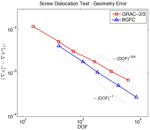
Figure 8. Convergence of the QNL-type GRAC-2/3 [20] and of the BGFC schemes for an anti-plane screw dislocation problem.

4.3. Complex crystals

To formulate the BGFC scheme for complex crystals, we return to the point defect problem adressed in § 2.

4.3.1. Atomistic model

Each lattice site may now contain more than one atom (of the same or different species). For simplicity suppose there are two atoms per site, which we call species 1 and species 2. The deformation of the lattice is now described by a deformation field $y:\Lambda\to\mathbb{R}^{d}$ and a shift $p:\Lambda\to\mathbb{R}^{d}$. The deformed positions of species 1 are given by $y_{1}(a):=y(a)$ and those of species 2 by $y_{2}(a):=y(a)+p(a)$, $a\in\Lambda$. Let ${\bf y}:=(y,p)$. The site energy is now a function

$$\Phi_{a}({\bf y})=\Phi_{a}\Big{(}\big{(}y_{i}(b)-y_{j}(a)\big{)}_{\begin{subarray}{c}i,j=1,2\\ b\in\Lambda\end{subarray}}\Big{)}.$$

At present there exists no published regularity theory for complex lattice defects corresponding to [7], which we employed in the discussion in § 2, and the following discussion is therefore based on unpublished notes [18, 16] and reasonable assumptions.

Let $\Phi_{a}^{\rm hom}$ be the site energy potential for the defect-free lattice, then we assume that there is an equilibrium shift $p_{0}$ such that ${\bf x}:=(x,p_{0})$ is a stable equilibrium configuration. By this, we mean that, for all ${\bf v}=(v,r)$ with $v,r:\Lambda^{\rm hom}\to\mathbb{R}^{d}$ compactly supported,

$$\sum_{a\in\Lambda}\langle\delta\Phi_{a}({\bf x}),{\bf v}\rangle=0\quad\text{and}\quad\sum_{a\in\Lambda}\big{\langle}\delta^{2}\Phi_{a}({\bf x}){\bf v},{\bf v}\big{\rangle}\geq c_{0}\big{(}|v|_{\mathscr{U}}^{2}+\|r\|_{\ell^{2}}^{2}\big{)};$$

that is, the configuration must also be stable under perturbations of the shifts. This corresponds in fact to the classical notion of stability in complex lattices; see [6] and references therein.

Then we define the energy difference functional

$$\mathscr{E}^{\rm a}({\bf u}):=\sum_{a\in\Lambda}\Phi_{a}^{\prime}({\bf u}),\qquad\text{where}\quad\Phi_{a}^{\prime}({\bf u}):=\Phi_{a}({\bf x}+{\bf u})-\Phi_{a}({\bf x}).$$

It can again be shown that $\mathscr{E}^{\rm a}$ is well-defined and regular on the space [16]

$${\bf U}:=\big{\{}{\bf v}=(v,r):\Lambda\to\mathbb{R}^{2d}\,\big{|}\,v\in\mathscr{U},r\in\ell^{2}\big{\}}.$$

The exact atomistic problem now reads

$${\bf u}^{\rm a}\in\arg\min\big{\{}\mathscr{E}^{\rm a}({\bf u})\,\big{|}\,{\bf u}\in{\bf U}\big{\}}.$$

4.3.2. The BGFC scheme

To define the BQCE and BGFC schemes, we first define the Cauchy–Born energy density by

$${\bf W}({\sf F},p):=\det{\sf A}^{-1}\Phi_{0}^{\rm hom}\big{(}({\sf F}x,p)\big{)},$$

where $\Phi_{a}^{\rm hom}$ is the site energy potential for the defect-free lattice. Further, let $W^{\prime}({\sf G},q):=W({\sf I}+{\sf G},p_{0}+q)-W({\sf I},p_{0})$.

Let the computational geometry be set up precisely as in § 2.4, and let

$${\bf U}_{h}:=\big{\{}{\bf u}_{h}=(u_{h},q_{h})\,\big{|}\,u_{h},q_{h}\in\mathscr{U}_{h}\big{\}}.$$

Note that, contrary to the usual practice, we require that both displacement and shift are continuous functions. This is necessary in order to be able to reconstruct atom positions. The BQCE energy functional, as proposed in [18], is given, for ${\bf u}_{h}=(u_{h},q_{h})\in{\bf U}_{h}$, by

$${\bf E}^{\rm b}({\bf u}_{h}):=\sum_{a\in\Lambda}(1-\beta(a))\Phi_{a}^{\prime}({\bf u}_{h})+\int_{{\Omega_{h}}}Q_{h}\big{[}\beta W^{\prime}(\nabla u_{h},q_{h})\big{]}\,{\rm d}x.$$

Because of the loss of point symmetry in the interaction potential there is also a reduction in the accuracy of the Cauchy–Born model [6] and in the blending scheme. Indeed, the analysis in [18] suggests that the best possible error that can be expected for the complex lattice BQCE method is

$$\|\nabla\overline{u^{\rm a}}-\nabla u_{h}^{\rm b}\|_{L^{2}}+\|p^{\rm a}-p_{h}^{\rm b}\|_{\ell^{2}}\lesssim\|\nabla\beta\|_{L^{2}}+\text{best approx. err.}+\text{CB err.},$$

that is the blended ghost force error now scales like $\|\nabla\beta\|_{L^{2}}$. If $d=2$, then it can be easily seen that $\|\nabla\beta\|_{L^{2}}\gtrsim 1$ while for $d=3$, one even gets $\|\nabla\beta\|_{L^{2}}\gtrsim(R^{\rm a})^{1/2}$. Thus, the standard BQCE scheme cannot be optimised to become convergent in the energy-norm.

To formulate the BGFC scheme, we renormalise $\Phi_{a}$ and $W$ a second time,

$$\Phi_{a}^{\prime\prime}({\bf u}) :=\Phi_{a}({\bf x}+{\bf u})-\Phi_{a}({\bf x})-\langle\delta\Phi_{a}({\bf x}),{\bf u}\rangle,\quad\text{and}$$

$${\bf W}^{\prime\prime}({\sf G},q) :=W({\sf I}+{\sf G},p_{0}+q)-W({\sf I},p_{0})-\partial_{\sf F}W({\sf I},p_{0}):{\sf G}-\partial_{p}W({\sf I},p_{0})\cdot q,$$

and define the BGFC energy functional

$${\bf E}^{\rm rb}({\bf u}):=\sum_{a\in\Lambda}(1-\beta(a))\Phi_{a}^{\prime\prime}({\bf u})+\int_{{\Omega_{h}}}Q_{h}\big{[}\beta W^{\prime\prime}(\nabla u,q)\big{]}\,{\rm d}x+\langle{\bf L}^{\rm ren},\bf u\rangle,$$

where ${\bf L}^{\rm ren}$ is a suitable linear functional correcting the forces in the defect core, defined analogously as $L^{\rm ren}$ in § 2.6. The BGFC scheme reads

$${\bf u}_{h}^{\rm rb}\in\arg\min\big{\{}{\bf E}^{\rm rb}({\bf v})\,\big{|}\,{\bf v}\in{\bf U}_{h}\big{\}}.$$ (4.1)

4.3.3. Convergence rate

While we leave a rigorous convergence theory for (4.1) to future work, we can still speculate what rate of convergence may be expected.

Arguing analogously as in § 2.6 and § 5 we now observe that the error due to the blended ghost forces can be bounded by

$$\|\nabla\overline{u^{\rm a}}-\nabla u_{h}^{\rm rb}\|_{L^{2}}+\|\overline{p^{\rm a}}-p_{h}^{\rm rb}\|_{L^{2}} \lesssim\|\nabla\beta\|_{L^{\infty}}\big{(}\|\nabla u^{\rm a}\|_{L^{2}(\Omega^{\rm b})}+\|q^{\rm a}\|_{L^{2}(\Omega^{\rm b})}\big{)}$$

$$\qquad+\text{best approx. err.}+\text{CB err.}.$$

It is reasonable to expect that the regularity for the deformation fields $y_{1},y_{2}$ is similar as for simple lattices and therefore the best approximation error is of the same order, i.e., $(R^{\rm a})^{-d}$. The Cauchy–Born modelling error can also be bounded by $\|\nabla^{2}\widetilde{u^{\rm a}}\|_{L^{2}(\mathbb{R}^{d}\setminus B_{R^{\rm a}})}+\|\nabla\widetilde{p^{\rm a}}\|_{L^{2}(\mathbb{R}^{d}\setminus B_{R^{\rm a}})}\lesssim(R^{\rm a})^{-d}$, where we assumed again the same regularity for complex lattice displacement fields as for the simple lattice case. (Since the shift itself is a gradient, it is reasonable to assume that $\nabla\widetilde{p^{\rm a}}$ decays like a second gradient.)

Thus, we are left to discuss the error due to the ghost forces. Assuming the typical decay for point defects, $|\nabla\widetilde{u^{\rm a}}|+|q^{\rm a}|\lesssim|x|^{-d}$ we obtain that, for a quasi-optimal choice of $\beta$, satisfying $\|\nabla\beta\|_{L^{\infty}}\lesssim(R^{\rm b}-R^{\rm a})^{-1}$,

$$\|\nabla\beta\|_{L^{\infty}}\big{(}\|\nabla u^{\rm a}\|_{L^{2}(\Omega^{\rm b})}+\|q^{\rm a}\|_{L^{2}(\Omega^{\rm b})}\big{)}\lesssim(R^{\rm b}-R^{\rm a})^{-1}(R^{\rm a})^{-d/2}.$$

Upon choosing $R^{\rm b}-R^{\rm a}\approx R^{\rm a}$, this yields the rates

$$\|\nabla\beta\|_{L^{\infty}}\big{(}\|\nabla u^{\rm a}\|_{L^{2}(\Omega^{\rm b})}+\|q^{\rm a}\|_{L^{2}(\Omega^{\rm b})}\big{)}\lesssim\left\{\begin{array}[]{rl}(R^{\rm a})^{-2},&d=2,\\ (R^{\rm a})^{-5/2},&d=3,\end{array}\right.$$

which is the best approximation rate for $d=2$ and a slightly reduced rate for $d=3$.

We therefore conclude that the expected rate of convergence for the complex lattice BGFC scheme, for point defects, is

$$\|\nabla\overline{u^{\rm a}}-\nabla u_{h}^{\rm rb}\|_{L^{2}}+\|\overline{p^{\rm a}}-p_{h}^{\rm rb}\|_{\ell^{2}}\lesssim\left\{\begin{array}[]{rl}(R^{\rm a})^{-2}\approx({\rm DOF})^{-1},&d=2,\\ (R^{\rm a})^{-5/2}\approx({\rm DOF})^{-5/6},&d=3.\end{array}\right.$$

With these heuristics in mind, we expect that it would be relatively straightforward to generalize the analysis in [9] and § 5 and thus obtain the first rigorously convergent a/c coupling scheme for complex crystals.

5. Analysis

For our rigorous error estimates we focus on a simplified point defect problem, following [9]. We shall cite several results that are summarized in [9] but drawn from other sources, but for the sake of convenience we will only cite [9] as a reference. A range of generalizations are possible but require some additional work, and in particular a more complex notation.

We assume $\Lambda\equiv\Lambda^{\rm hom}$, with globally homogeneous site energies with a finite interaction radius in reference configuration. That is, we assume that there exists $\mathcal{R}\subset B_{r_{\rm cut}}\cap(\Lambda\setminus\{0\})$, finite, and $V\in C^{4}((\mathbb{R}^{d})^{\mathcal{R}})$ such that $\Phi_{a}(y)=V(Dy(a))$, where $Dy(a):=(D_{\rho}y(a))_{\rho\in\mathcal{R}}$ and $D_{\rho}y(a):=y(a+\rho)-y(a)$. We assume throughout that $V$ is point symmetric, i.e., $-\mathcal{R}=\mathcal{R}$ and $V((-g_{-\rho}))=V((g_{\rho}))$ for all $(g_{\rho})_{\rho\in\mathcal{R}}\in(\mathbb{R}^{d})^{\mathcal{R}}$.

A defect is introduced by adding an external potential $\mathscr{P}^{\rm def}\in C^{2}(\mathscr{U})$, which only depends on $Du(a),|a|<R^{\rm def}$. The atomistic problem now reads

$$u^{\rm a}\in\arg\min\big{\{}\mathscr{E}^{\rm a}(v)+\mathscr{P}^{\rm def}(v)\,\big{|}\,v\in\mathscr{U}\big{\}}.$$ (5.1)

We call a point $u^{\rm a}$ a strongly stable solution to (5.1) if there exists $\gamma>0$ such that

$$\langle\delta[\mathscr{E}^{\rm a}+\mathscr{P}^{\rm def}](u^{\rm a}),v\rangle=0\quad\text{and}\quad\langle\delta^{2}[\mathscr{E}^{\rm a}+\mathscr{P}^{\rm def}](u^{\rm a})v,v\rangle\geq\gamma|v|_{\mathscr{U}}^{2}\quad\forall v\in\mathscr{U}.$$

The BGFC approximation to (5.1) is given by

$$u^{\rm bg}_{h}\in\arg\min\big{\{}\mathscr{E}^{\rm bg}(v_{h})+\mathscr{P}^{\rm def}(v_{h})\,\big{|}\,v_{h}\in\mathscr{U}_{h}\big{\}},$$ (5.2)

using the notations of § 2.6.

5.1. Additional assumptions

We now summarize the main assumptions we require to state our rigorous convergence results. All assumptions can be satisfied in practice, and are discussed in detail in [9].

We assume that $\beta\in C^{2,1}(\mathbb{R}^{d})$, $0\leq\beta\leq 1$. Let $r_{\rm cut}^{\prime}:=2r_{\rm cut}+\sqrt{d}$, $\Omega^{\rm a}:={\rm supp}(1-\beta)+B_{r_{\rm cut}^{\prime}}$, $\Omega^{\rm b}:={\rm supp}(\nabla\beta)+B_{r_{\rm cut}^{\prime}}$ and $\Omega^{\rm c}:=({\rm supp}(\beta)+B_{r_{\rm cut}^{\prime}})\cap{\Omega_{h}}$. Then we require that there exist radii $R^{\rm a}\leq R^{\rm b}\leq R^{\rm c}$ and constants $C_{\rm b},C_{\Omega}$ such that

$$R^{\rm b}\leq C_{\rm b}R^{\rm a},\qquad\|\nabla^{j}\beta\|_{L^{\infty}}\leq C_{\rm b}(R^{\rm a})^{-j},j=1,2,3;$$

$${\rm supp}(\beta)\supset B_{R^{\rm a}+r_{\rm cut}^{\prime}},\qquad{\rm supp}(1-\beta)\subset B_{R^{\rm b}-r_{\rm cut}^{\prime}};$$

$$B_{R^{\rm c}}\subset\Omega^{\rm a}\cup\Omega^{\rm c}\qquad\text{and}\qquad R^{\rm c}\geq C_{\Omega}(R^{\rm a})^{2}.$$

To state the final assumption that we require on $\mathcal{T}_{h}$, we first need to define a piecewise affine interpolant of lattice functions.

The first is a piecewise affine interpolant. If $d=2$, let $\hat{\mathcal{T}}:=\{\hat{T}_{1},\hat{T}_{2}\}$, where $\hat{T}_{1}={\rm conv}\{0,e_{1},e_{2}\}$ and $\hat{T}_{2}={\rm conv}\{e_{1},e_{2},e_{1}+e_{2}\}$, where ${\rm conv}$ denotes the convex hull of a set of points. If $d=3$, let $\hat{\mathcal{T}}:=\{\hat{T}_{1},\dots,\hat{T}_{6}\}$ be the standard subdivision of $[0,1]^{3}$ into six tetrahedra (see [9, Fig. 1]). Then $\mathcal{T}:=\bigcup_{\ell\in\Lambda}(\ell+\hat{\mathcal{T}})$ defines a regular and uniform triangulation of $\mathbb{R}^{d}$ with node set $\Lambda$. For each $v:\Lambda\to\mathbb{R}^{m}$, there exists a unique $\bar{v}\in C(\mathbb{R}^{d};\mathbb{R}^{m})$ such that $\bar{v}(\ell)=v(\ell)$ for all $\ell\in\Lambda$. In particular, we note that the semi-norms $\|\nabla\bar{v}\|_{L^{2}}$ and $|v|_{\mathscr{U}}$ are equivalent.

Our final requirement on the approximation parameters is that there exists a constant $C_{h}$ such that

$$\mathcal{T}_{h}\cap\Omega^{\rm a}\equiv\mathcal{T}\cap\Omega^{\rm a}\qquad\qquad\max_{T\in\mathcal{T}_{h}}h_{T}^{d}/|T|\leq C_{h},$$

$$h(x)\leq C_{h}\max\big{(}1,|x|/R^{\rm a}\big{)}\qquad\text{and}\qquad\#\mathcal{T}_{h}\leq C_{h}(R^{\rm a})^{2}\log(R^{\rm a}).$$

By $\mathcal{T}_{h}\cap\Omega^{\rm a}\equiv\mathcal{T}\cap\Omega^{\rm a}$ we mean that, if $T\in\mathcal{T},T\cap\Omega^{\rm a}\neq\emptyset$ then $T\in\mathcal{T}_{h}$ (and hence also vice-versa). The condition $h(x)\leq C_{h}\max\big{(}1,|x|/R^{\rm a}\big{)}$ can be weakened; see e.g. [13, 19].

We remark that $(\beta,\mathcal{T}_{h})$ are the main approximation parameters, while the “regularity constants” ${\bf C}=(C_{\rm b},C_{h},C_{\Omega})$ are “derived parameters”. In the following we fix the constants ${\bf C}$ to some given bounds, and admit any pair $(\beta,\mathcal{T}_{h})$ satisfying the foregoing conditions with these constants. When we write $A\lesssim B$, then we mean that there exists a constant $C$ depending only on ${\bf C}$ (as well as on the solution and on the model) but not on $(\beta,\mathcal{T}_{h})$ such that $A\leq CB$.

5.2. Convergence result

The following convergence result is a direct extension of Theorem 3.1, Proposition 3.2 and Theorem 3.3 in [9] to the BGFC method. The proof of the theorem is given in the next two sections.

Theorem 5.1. Let $u^{\rm a}$ be a strongly stable solution to (5.1), then for any given set of constants ${\bf C}$ there exist $C,C^{\prime},R^{\rm a}_{0}>0$ such that, for all $(\beta,\mathcal{T}_{h})$ satisfying the conditions of § 5.1, and in addition $R^{\rm a}\geq R^{\rm a}_{0}$, there exists a solution $u^{\rm bg}_{h}$ to (5.2) such that

$$\|\nabla\overline{u^{\rm a}}-\nabla u^{\rm bg}_{h}\|_{L^{2}} \leq C(R^{\rm a})^{-d/2-1}\leq C^{\prime}\big{(}{\textstyle\frac{\log\#\mathcal{T}_{h}}{\#\mathcal{T}_{h}}}\big{)}^{1/2+1/d},\qquad\text{and}$$ (5.3)

$$\big{|}\mathscr{E}^{\rm a}(u^{\rm a})-\mathscr{E}^{\rm bg}(u^{\rm bg}_{h})\big{|} \leq C(R^{\rm a})^{-d-2}\leq C^{\prime}\big{(}{\textstyle\frac{\log\#\mathcal{T}_{h}}{\#\mathcal{T}_{h}}}\big{)}^{1+2/d}.$$ (5.4)

Remark 3. 1. The only assumption we made that represents a genuine restriction of generality is that $\|\nabla^{j}\beta\|_{L^{\infty}}\lesssim(R^{\rm a})^{-j}$. We require this to prove stability of the BQCE and BGFC schemes.

2. However, the proof of (5.4) shows that the energy error would be sub-optimal if we chose a narrower blending region (and thus a slower rate of $\|\nabla^{j}\beta\|_{L^{\infty}}\lesssim(R^{\rm a})^{-sj}$ for some $s<1$). This appears to contradict our numerical results in § 3 and suggests that the energy error estimate may be suboptimal. ∎

5.3. Proof of the energy norm error estimate

To prove the result we will need to refer to another technical tool from [9], namely a $C^{2,1}$-conforming multi-quintic, which we use to measure the regularity of an atomistic displacement.

For $v:\Lambda\to\mathbb{R}^{m}$ and $i=1,\dots,d$, let ${\sf d}_{i}^{0}v(\ell):=v(\ell)$; ${\sf d}_{i}^{1}v(\ell):=\frac{1}{2}(u(\ell+e_{i})-u(\ell-e_{i}))$ and ${\sf d}_{i}^{2}v(\ell):=u(\ell+e_{i})-2u(\ell)+u(\ell-e_{i})$. Lemma 2.1 in [9] states that, for each $\ell\in\Lambda$ there exists a unique multi-quintic function $\tilde{v}:\ell+[0,1]^{d}\to\mathbb{R}^{m}$ defined through the conditions

$$\partial_{x_{1}}^{\alpha_{1}}\cdots\partial_{x_{d}}^{\alpha_{d}}\tilde{v}(\ell^{\prime})={\sf d}_{1}^{\alpha_{1}}\cdots{\sf d}_{d}^{\alpha_{d}}v(\ell^{\prime})\qquad\forall\ell^{\prime}\in\ell+\{0,1\}^{d},\alpha\in\{0,1,2\}^{d},\|\alpha\|_{\infty}\leq 2,$$

and moreover, that the resulting piecewise defined function on $\mathbb{R}^{d}$ belongs to $\tilde{v}\in C^{2,1}(\mathbb{R}^{d};\mathbb{R}^{m})$.

We begin the proof of Theorem 5.2 by noting that the renormalised site energy potential

$$V^{\prime\prime}(Du):=V(\mathcal{R}+Du)-V(\mathcal{R})-\langle\delta V(\mathcal{R}),Du\rangle$$

is an admissible potential for [9, Thm. 3.1]. Further, the conditions we put forward in § 5.1 are precisely those we need to apply [9, Thm. 3.1] with $V$ replaced with $V^{\prime\prime}$, thus treating BGFC as a simple BQCE method. Hence, we obtain that, under the conditions of Theorem 5.2, there exists a solution $u^{\rm bg}_{h}$ to (5.2) and constants $C_{1},C_{2}$ depending only on ${\bf C}$, but independent of the approximation parameters, such that

$$\|\nabla\overline{u^{\rm a}}-\nabla u^{\rm bg}_{h}\|_{L^{2}}\leq C_{1}\|\nabla^{2}\beta\|_{L^{2}}+C_{2}\Big{(} ~{}\|\nabla\bar{u}^{\rm a}\|_{L^{2}(\mathbb{R}^{2}\setminus B_{R^{\rm c}/2})}+\|h\nabla^{2}\tilde{u}^{\rm a}\|_{L^{2}(\Omega^{\rm c})}$$

$$+\|h^{2}\nabla^{3}\tilde{u}^{\rm a}\|_{L^{2}(\Omega^{\rm c})}+\|\nabla^{2}\tilde{u}^{\rm a}\|_{L^{4}(\Omega^{\rm c})}^{2}\Big{)}.$$ (5.5)

Here we did not write out some terms that are trivially dominated by those that we did write. In the following we write $u\equiv u^{\rm a}$.

The group preceded by the constant $C_{2}$ cannot be further improved, but we will analyse in more detail the group $C_{1}\|\nabla^{2}\beta\|_{L^{2}}$. This term arises from the coarsening and modelling error analysis of the BQCE scheme in § 6.1 and § 6.2 of [9] (see also the summary in §4.3 of [9]). We can replace $C_{1}\|\nabla^{2}\beta\|$ in (5.5) with two terms $\epsilon_{\beta}^{\rm coarse}+\epsilon_{\beta}^{\rm model}$, which we discuss next, to obtain

$$\|\nabla\bar{u}-\nabla u^{\rm bg}_{h}\|_{L^{2}}\leq\epsilon_{\beta}^{\rm coarse}+\epsilon_{\beta}^{\rm model}+C_{2}\Big{(} ~{}\|\nabla\bar{u}\|_{L^{2}(\mathbb{R}^{2}\setminus B_{R^{\rm c}/2})}+\|h\nabla^{2}\tilde{u}\|_{L^{2}(\Omega^{\rm c})}$$

$$+\|h^{2}\nabla^{3}\tilde{u}\|_{L^{2}(\Omega^{\rm c})}+\|\nabla^{2}\tilde{u}\|_{L^{4}(\Omega^{\rm c})}^{2}\Big{)}.$$ (5.6)

From Lemma 6.1 and Lemma 6.2 of [9] it can be readily seen that the coarsening error contribution to $C_{1}\|\nabla^{2}\beta\|_{L^{2}}$ is

$$\epsilon_{\beta}^{\rm coarse}\lesssim\|\partial W^{\prime\prime}({\sf I}+\nabla\tilde{u})\nabla^{2}\beta\|_{L^{2}}.$$

Using that fact that $\partial W^{\prime\prime}({\sf I})=0$ (due to the renormalisation, the reference configuration is now stress free) we therefore obtain

$$\epsilon_{\beta}^{\rm coarse}\lesssim\big{\|}\big{[}\partial W^{\prime\prime}({\sf I}+\nabla\tilde{u})-\partial W^{\prime\prime}({\sf I})\big{]}\nabla^{2}\beta\big{\|}_{L^{2}}\lesssim\big{\|}\,|\nabla\tilde{u}|\,|\nabla^{2}\beta|\,\big{\|}_{L^{2}}.$$ (5.7)

To obtain a more precise control on the modelling error contribution we first take a closer look at the term ${\rm T}_{1}$ defined in Equation (6.6) in [9],

$${\rm T}_{1}=\beta\partial W^{\prime\prime}-\sum_{\ell\in\Lambda}\beta(\ell)\sum_{\rho\in\mathcal{R}}\big{[}V_{,\rho}^{\prime\prime}\otimes\rho\big{]}\omega_{\rho}(\ell-x),$$

where $\partial W^{\prime\prime}=\partial W^{\prime\prime}({\sf I}+\nabla\tilde{u}(x))$, $V_{,\rho}^{\prime\prime}=V_{,\rho}^{\prime\prime}(({\sf I}+\nabla\tilde{u}(x))\mathcal{R})$ and $\omega_{\rho}(y)=\int_{s=0}^{1}\bar{\zeta}(y+s\rho)\,{\rm d}s$, with $\bar{\zeta}$ being the P1 hat function for the origin on the mesh $\mathcal{T}$. The $O(\|\nabla^{2}\beta\|)$ term now arises by expanding $\beta$,

$$\beta(\ell)=\beta(x)+\nabla\beta(x)\cdot(\ell-x)+R_{\beta}(x;\ell),$$

with $|R_{\beta}(x;\ell)|\lesssim\|\nabla^{2}\beta\|_{L^{\infty}}$ due to the fact that only $\ell$ within a fixed radius around $x$ are considered in the seemingly infinite sum. Thus, exploiting also the fact that $V^{\prime\prime}_{,\rho}(\mathcal{R})\equiv 0$ and $\sum_{\ell\in\Lambda}\omega_{\rho}(\ell-x)=1$ (see [9, Eq. (4.18)]), and denoting the terms that lead to the second group in (5.6) by “$\cdots$”, we obtain

$$|{\rm T}_{1}| \leq\|\nabla^{2}\beta\|_{L^{\infty}}\sum_{\rho\in\mathcal{R}}\Big{|}\big{(}V_{,\rho}^{\prime\prime}(\mathcal{R}+\nabla\tilde{u})-V_{,\rho}^{\prime\prime}(\mathcal{R})\big{)}\otimes\rho\sum_{\ell\in\Lambda}\omega_{\rho}(\ell-x)\Big{|}+\dots$$

$$\lesssim\|\nabla^{2}\beta\|_{L^{\infty}}\sum_{\rho\in\mathcal{R}}\big{|}V_{,\rho}^{\prime\prime}(\mathcal{R}+\nabla\tilde{u})-V_{,\rho}^{\prime\prime}(\mathcal{R})\big{|}+\dots$$

$$\lesssim\|\nabla^{2}\beta\|_{L^{\infty}}|\nabla\tilde{u}(x)|+\dots.$$

The improved modelling error estimate is obtained by taking the $L^{2}$-norm of ${\rm T}_{1}$, interpreting it as a function of $x$. Upon noting that ${\rm T}_{1}(x)=0$ outside $\Omega^{\rm b}$, we therefore obtain

$$\epsilon_{\beta}^{\rm model}\lesssim\|\nabla^{2}\beta\|_{L^{\infty}}\|\nabla\tilde{u}\|_{L^{2}(\Omega^{\rm b})}.$$ (5.8)

Combining (5.6), (5.7) and (5.8) we arrive at

$$\|\nabla\bar{u}-\nabla u^{\rm bg}_{h}\|_{L^{2}} \leq C\Big{(}\|\nabla^{2}\beta\|_{L^{\infty}}\|\nabla\tilde{u}\|_{L^{2}(\Omega^{\rm b})}+\|\nabla\bar{u}\|_{L^{2}(\mathbb{R}^{2}\setminus B_{R^{\rm c}/2})}+\|h\nabla^{2}\tilde{u}\|_{L^{2}(\Omega^{\rm c})}$$

$$\qquad+\|h^{2}\nabla^{3}\tilde{u}\|_{L^{2}(\Omega^{\rm c})}+\|\nabla^{2}\tilde{u}\|_{L^{4}(\Omega^{\rm c})}^{2}\Big{)},$$ (5.9)

for a constant $C$ that depends only on ${\bf C}$, but is independent of $(\beta,\mathcal{T}_{h})$.

Following the proof of [9, Thm. 3.3] in §3.2.2 of [9] it is straightforward now to obtain the rate (5.3). Towards its proof we only remark that, according to [9, Lemma 2.3], $|\nabla\tilde{u}(x)|\lesssim|x|^{-d}$ and hence, using the assumption $\|\nabla^{2}\beta\|_{L^{\infty}}\lesssim(R^{\rm a})^{-2}$, we obtain

$$\|\nabla^{2}\beta\|_{L^{\infty}}\,\|\nabla\tilde{u}\|_{L^{2}(\Omega^{\rm b})}\lesssim(R^{\rm a})^{-2}\bigg{(}\int_{R^{\rm a}}^{R^{\rm b}}r^{d-1}r^{-2d}\,{\rm d}r\bigg{)}^{1/2}\lesssim(R^{\rm a})^{-2-d/2}.$$

This completes the proof of (5.3).

5.4. Proof of the energy error estimate

As in the case of the energy-norm error estimate we only modify some specific parts of the proof for the BQCE case in § 6.3 of [9], as required to obtain the improved energy error estimate. To follow the notation let $u\equiv u^{\rm a}$ and $u_{h}\equiv u^{\rm bg}_{h}$. Further, we recall that $\Pi_{h}u\in\mathscr{U}_{h}$ is a best-approximation of $u$. For the following proof we do not need to know its precise definition, but only remark that $\Pi_{h}u=u$ in $\Omega^{\rm a}$ and, as an intermediate step in the proof of (5.3) one obtains

$$\|\nabla\tilde{u}-\nabla\Pi_{h}u\|_{L^{2}(\Omega^{\rm c})}+\|\nabla u_{h}-\nabla\Pi_{h}u\|_{L^{2}}\lesssim(R^{\rm a})^{-1-d/2}.$$

Following the proof of the BQCE energy error estimate in § 6.3 of [9], we split the energy error into $\mathscr{E}^{\rm a}(u)-\mathscr{E}^{\rm bg}(u_{h})=T_{1}+T_{2}+T_{3}$, where

$$T_{1}=\mathscr{E}^{\rm a}(u)-\tilde{\mathcal{E}},\qquad T_{2}=\tilde{\mathcal{E}}-\mathscr{E}^{\rm bg}(\Pi_{h}u),\qquad T_{3}=\mathscr{E}^{\rm bg}(\Pi_{h}u)-\mathscr{E}^{\rm bg}(u_{h}),$$

$$\text{and }\tilde{\mathcal{E}}=\sum_{\ell\in\Lambda}(1-\beta(\ell))V^{\prime\prime}(Du(\ell))+\int_{\mathbb{R}^{d}}[Q_{h}\beta]W^{\prime\prime}(\nabla\tilde{u})\,{\rm d}x.$$

We treat the terms in the same order as in [9].

As in [9], the term $T_{3}$ can be bounded by

$$|T_{3}|\lesssim\|\nabla u_{h}-\nabla\Pi_{h}u\|_{L^{2}}\lesssim(R^{\rm a})^{-2-d}.$$ (5.10)

The term $T_{1}$ is split further into

$$T_{1} =\sum_{\ell\in\Lambda}\beta(\ell)\big{(}V^{\prime\prime}(Du(\ell))-W^{\prime\prime}(\nabla\tilde{u}(\ell))\big{)}$$

$$\qquad+\int_{\mathbb{R}^{d}}\big{(}[Q_{h}\beta]W^{\prime\prime}(\nabla\tilde{u})-I_{1}[\beta W^{\prime\prime}(\nabla\tilde{u})]\big{)}\,{\rm d}x=:T_{1,1}+T_{1,2},$$

where $I_{1}$ denotes the P1 nodal interpolant for the atomistic mesh $\mathcal{T}$. The second term is essentially a quadrature error and following the proof of (6.12) in [9] (but note that the inverse-estimate trick is not required in our present setting) it is easy to see that

$$|T_{1,2}|\lesssim\sum_{T\in\mathcal{T}}\|\nabla^{2}[\beta W^{\prime\prime}(\nabla\tilde{u})]\|_{L^{\infty}(T)}.$$

The summand vanishes, unless $T\subset\Omega^{\rm c}$. In the latter case, we have

$$\|\nabla^{2}[\beta W^{\prime\prime}(\nabla\tilde{u})]\|_{L^{\infty}(T)} \lesssim\|\nabla^{2}\beta\|_{L^{\infty}}\|\nabla\tilde{u}\|_{L^{2}(T)}^{2}+\|\nabla\beta\|_{L^{\infty}(T)}\|\partial W^{\prime\prime}(\nabla\tilde{u})\nabla^{2}\tilde{u}\|_{L^{\infty}(T)}$$

$$\qquad+\|\partial W^{\prime\prime}(\nabla\tilde{u})\nabla^{3}\tilde{u}\|_{L^{\infty}}+\|\partial^{2}W^{\prime\prime}(\nabla\tilde{u})\nabla^{2}\tilde{u}\|_{L^{\infty}(T)}^{2}$$

$$\lesssim\|\nabla^{2}\beta\|_{L^{\infty}}\|\nabla\tilde{u}\|_{L^{2}(T)}^{2}+\|\nabla\beta\|_{L^{\infty}}\|\nabla\tilde{u}\|_{L^{2}(T)}\|\nabla^{2}\tilde{u}\|_{L^{2}(T)}$$

$$\qquad+\|\nabla\tilde{u}\|_{L^{2}(T)}\|\nabla^{3}\tilde{u}\|_{L^{2}(T)}+\|\nabla^{2}\tilde{u}\|_{L^{2}(T)}^{2}.$$

Therefore, we obtain

$$|T_{1,2}| \lesssim\|\nabla^{2}\beta\|_{L^{\infty}}\|\nabla\tilde{u}\|_{L^{2}(\Omega^{\rm b})}^{2}+\|\nabla\beta\|_{L^{\infty}}\|\nabla\tilde{u}\|_{L^{2}(\Omega^{\rm b})}\|\nabla^{2}\tilde{u}\|_{L^{2}(\Omega^{\rm b})}$$

$$\qquad+\|\nabla\tilde{u}\|_{L^{2}(\Omega^{\rm c})}\|\nabla^{3}\tilde{u}\|_{L^{2}(\Omega^{\rm c})}+\|\nabla^{2}\tilde{u}\|_{L^{2}(\Omega^{\rm c})}^{2}$$ (5.11)

$$\lesssim(R^{\rm a})^{-2-d}+(R^{\rm a})^{-2-d}+(R^{\rm a})^{-2-d}+(R^{\rm a})^{-2-d}\approx(R^{\rm a})^{-2-d}.$$

To estimate $T_{1,1}$ we begin by noting that

$$V^{\prime\prime}(Du)-W^{\prime\prime}(\nabla u) =V^{\prime\prime}(\mathcal{R}+Du)-V^{\prime\prime}(\mathcal{R}+\nabla_{\mathcal{R}}u)$$

$$=\langle\delta V^{\prime\prime}(\mathcal{R}+\nabla_{\mathcal{R}}u),Du-\nabla_{\mathcal{R}}u\rangle$$

$$\qquad+\langle\delta^{2}V(\Theta)(Du-\nabla_{\mathcal{R}}u),Du-\nabla_{\mathcal{R}}u\rangle,$$

where $\Theta\in{\rm conv}\{\mathcal{R}+Du,\mathcal{R}+\nabla_{\mathcal{R}}u\}$ and $\nabla_{\mathcal{R}}u:=(\nabla_{\rho}u)_{\rho\in\mathcal{R}}$. Then, continuing to argue as in Lemma 6.5 and [9] (performing a Taylor expansion on $Du$ and exploiting the point symmetry of $V^{\prime\prime}$, and in particular exploiting the fact that $\|\delta V^{\prime\prime}(\mathcal{R}+\nabla_{\mathcal{R}}u)\|\lesssim|\nabla\tilde{u}|$) we obtain

$$\big{|}\langle\delta V^{\prime\prime}(\mathcal{R}+\nabla_{\mathcal{R}}u),Du-\nabla_{\mathcal{R}}u\rangle\big{|} \lesssim||\nabla u|\|\nabla^{3}\tilde{u}\|_{L^{\infty}(\nu_{x})},\quad\text{and}$$

$$\big{|}\langle\delta^{2}V(\Theta)(Du-\nabla_{\mathcal{R}}u),Du-\nabla_{\mathcal{R}}u\rangle\big{|} \lesssim\|\nabla^{2}\tilde{u}\|_{L^{\infty}(\nu_{x})}^{2},$$

where $\nu_{x}=B_{r_{\rm cut}^{\prime}}(x)$. Using the fact that $\nabla^{3}\tilde{u}$ is a piecewise polynomial we can use the inverse inequalities in (5.7) of [9] to obtain, as in (6.14) of [9], that

$$|T_{1,1}| \lesssim\|\nabla\tilde{u}\|_{L^{2}(\Omega^{\rm c})}\|\nabla^{3}\tilde{u}\|_{L^{2}(\Omega^{\rm c})}+\|\nabla^{2}\tilde{u}\|_{L^{2}(\Omega^{\rm c})}^{2}$$

$$\lesssim(R^{\rm a})^{-2-d}+(R^{\rm a})^{-2-d}\approx(R^{\rm a})^{-2-d}.$$ (5.12)

Since $\Pi_{h}u=u$ in $\Omega^{\rm a}$, the term $T_{2}$ simplifies to

$$T_{2}=\int_{\mathbb{R}^{d}}[Q_{h}\beta]\big{(}W^{\prime\prime}(\nabla\tilde{u})-W^{\prime\prime}(\nabla\tilde{u}-\nabla e)\big{)}\Big{)}\,{\rm d}x,$$

where $e:=\tilde{u}-\Pi_{h}u$ and we used the fact that $Q_{h}[\beta W^{\prime\prime}(\nabla\Pi_{h}u)]=[Q_{h}\beta]W^{\prime\prime}(\nabla\Pi_{h}u)$. We begin by expanding $W^{\prime\prime}(\nabla\tilde{u})-W^{\prime\prime}(\nabla\tilde{u}-\nabla e)=\partial W^{\prime\prime}(\nabla\tilde{u}):\nabla e+O(|\nabla e|^{2})$ to obtain

$$T_{2} \lesssim\bigg{|}\int_{\mathbb{R}^{d}}[Q_{h}\beta]\big{[}\partial W^{\prime\prime}(\nabla\tilde{u}):\nabla e\big{]}\,{\rm d}x\bigg{|}+\|\nabla e\|_{L^{2}(\Omega^{\rm c})}^{2}$$

$$\lesssim\bigg{|}\int_{\mathbb{R}^{d}}\beta\big{[}\partial W^{\prime\prime}(\nabla\tilde{u}):\nabla e\big{]}\,{\rm d}x\bigg{|}+\bigg{|}\int_{\mathbb{R}^{d}}[Q_{h}\beta-\beta]\big{[}\partial W^{\prime\prime}(\nabla\tilde{u}):\nabla e\big{]}\,{\rm d}x\bigg{|}$$

$$\qquad+\|\nabla e\|_{L^{2}(\Omega^{\rm c})}^{2}\lesssim T_{2,1}+T_{2,2}+T_{2,3}.$$

To treat $T_{2,1}$ we integrate by parts, and then use $|\partial W^{\prime\prime}(\nabla\tilde{u})|=|\partial W({\sf I}+\nabla\tilde{u})-\partial W({\sf I})|\lesssim|\nabla\tilde{u}|$, $\|e\|_{L^{2}(T)}\lesssim\|h^{2}\nabla^{2}\tilde{u}\|_{L^{2}(T)}$, and $\|h^{2}\nabla^{2}\tilde{u}\|_{L^{2}(\Omega^{\rm c})}\lesssim(R^{\rm a})^{-1-d/2}$ to estimate

$$T_{2,1} =\bigg{|}\int_{\mathbb{R}^{d}}-{\rm div}\Big{(}\beta\partial W^{\prime\prime}(\nabla\tilde{u})\Big{)}\cdot e\,{\rm d}x\bigg{|}$$

$$\lesssim\|\nabla\beta\|_{L^{\infty}}\|\partial W^{\prime\prime}(\nabla\tilde{u})\|_{L^{2}(\Omega^{\rm c})}\|e\|_{L^{2}(\Omega^{\rm c})}+\|\nabla^{2}\tilde{u}\|_{L^{2}(\Omega^{\rm c})}\|e\|_{L^{2}(\Omega^{\rm c})}$$

$$\lesssim\|\nabla\beta\|_{L^{\infty}}\|\nabla\tilde{u}\|_{L^{2}(\Omega^{\rm c})}\|e\|_{L^{2}(\Omega^{\rm c})}+\|\nabla^{2}\tilde{u}\|_{L^{2}(\Omega^{\rm c})}\|e\|_{L^{2}(\Omega^{\rm c})}$$

$$\lesssim(R^{\rm a})^{-1}(R^{\rm a})^{-d/2}(R^{\rm a})^{-1-d/2}+(R^{\rm a})^{-1-d/2}(R^{\rm a})^{-1-d/2}\approx(R^{\rm a})^{-2-d}.$$

The terms $T_{2,2}$ and $T_{2,3}$ are estimated analogously, by $T_{2,j}\lesssim(R^{\rm a})^{-2-d}$, $j=2,3$, and thus we obtain that

$$|T_{2}|\lesssim(R^{\rm a})^{-2-d}.$$ (5.13)

Combining (5.10), (5.11), (5.12) and (5.13) completes the proof of (5.4).

References

- [1] M. S. Daw and M. I. Baskes. Embedded-Atom Method: Derivation and Application to Impurities, Surfaces, and other Defects in Metals. Physical Review B, 20, 1984.
- [2] A. Dedner, C. Ortner, and H. Wu. work in progress.
- [3] M. Dobson and M. Luskin. Analysis of a force-based quasicontinuum approximation. M2AN Math. Model. Numer. Anal., 42(1):113–139, 2008.
- [4] M. Dobson, M. Luskin, and C. Ortner. Stability, instability, and error of the force-based quasicontinuum approximation. Arch. Ration. Mech. Anal., 197(1):179–202, 2010.
- [5] W. E, J. Lu, and J. Z. Yang. Uniform accuracy of the quasicontinuum method. Phys. Rev. B, 74(21):214115, 2006.
- [6] W. E and P. Ming. Cauchy-Born rule and the stability of crystalline solids: static problems. Arch. Ration. Mech. Anal., 183(2):241–297, 2007.
- [7] V. Ehrlacher, C. Ortner, and A. V. Shapeev. Analysis of boundary conditions for crystal defect atomistic simulations. ArXiv e-prints, 1306.5334v1, 2013.
- [8] X. H. Li, M. Luskin, C. Ortner, and A. V. Shapeev. Theory-based benchmarking of blended force-based quasicontinuum method. Comp. Meth. Appl. Mech. Engrg, 268:763–781, 2014.
- [9] X. H. Li, C. Ortner, A. V. Shapeev, and B. Van Koten. Analysis of blended atomistic/continuum hybrid methods. ArXiV e-prints, 1404.4878, 2014.
- [10] J. Lu and P. Ming. Stability of a force-based hybrid method in three dimension with sharp interface. ArXiv e-prints, December 2012.
- [11] J. Lu and P. Ming. Convergence of a force-based hybrid method in three dimensions. Comm. Pure Appl. Math., 66(1):83–108, 2013.
- [12] M. Luskin and C. Ortner. Atomistic-to-continuum-coupling. Acta Numerica, 2013.
- [13] M. Luskin, C. Ortner, and B. Van Koten. Formulation and optimization of the energy-based blended quasicontinuum method. Comput. Methods Appl. Mech. Engrg., 253, 2013.
- [14] C. Makridakis, C. Ortner, and E. Süli. A priori error analysis of two force-based atomistic/continuum hybdrid models of a periodic chain. OxMOS Report No. 28/2010.
- [15] D. Olson, P. Bochev, M. Luskin, and A. V. Shapeev. Development of an optimization-based atomistic-to-continuum coupling method. ArXiv e-prints, 1309.5988, 2013.
- [16] C. Ortner. work in progress.
- [17] C. Ortner. The role of the patch test in 2D atomistic-to-continuum coupling methods. arXiv:1101.5256v2.
- [18] C. Ortner and B. Van Koten. work in progress.
- [19] C. Ortner and A. V. Shapeev. Analysis of an Energy-based Atomistic/Continuum Coupling Approximation of a Vacancy in the 2D Triangular Lattice. Math. Comp., 82, 2013.
- [20] C. Ortner and L. Zhang. Construction and sharp consistency estimates for atomistic/continuum coupling methods with general interfaces: a 2D model problem. SIAM J. Numer. Anal., 50, 2012.
- [21] C. Ortner and L. Zhang. Energy-based atomisitic-to-continuum coupling without ghost forces. ArXiv e-prints, 1312.6814, 2013.
- [22] V. B. Shenoy, R. Miller, E. B. Tadmor, D. Rodney, R. Phillips, and M. Ortiz. An adaptive finite element approach to atomic-scale mechanics–the quasicontinuum method. J. Mech. Phys. Solids, 47(3):611–642, 1999.
- [23] T. Shimokawa, J. J. Mortensen, J. Schiotz, and K. W. Jacobsen. Matching conditions in the quasicontinuum method: Removal of the error introduced at the interface between the coarse-grained and fully atomistic region. Phys. Rev. B, 69(21):214104, 2004.
- [24] B. Van Koten and M. Luskin. Analysis of energy-based blended quasi-continuum approximations. SIAM J. Numer. Anal., 49(5):2182–2209, 2011.
- [25] S. P. Xiao and T. Belytschko. A bridging domain method for coupling continua with molecular dynamics. Comput. Methods Appl. Mech. Engrg., 193(17-20):1645–1669, 2004.