Posterior predictive checks to quantify lack-of-fit in admixture models of latent population structure
David Mimno1, David M Blei2, Barbara E Engelhardt3,∗
1 Department of Information Science, Cornell University
2 Departments of Statistics and Computer Science, Columbia University
3 Departments of Biostatistics & Bioinformatics and Statistical Science, Duke University
E-mail: barbara.engelhardt@duke.edu
Abstract
Admixture models are a ubiquitous approach to capture latent population structure in genetic samples. Despite the widespread application of admixture models, little thought has been devoted to the quality of the model fit or the accuracy of the estimates of parameters of interest for a particular study. Here we develop methods for validating admixture models based on posterior predictive checks (PPCs), a Bayesian method for assessing the quality of a statistical model. We develop PPCs for five population-level statistics of interest: within-population genetic variation, background linkage disequilibrium, number of ancestral populations, between-population genetic variation, and the downstream use of admixture parameters to correct for population structure in association studies. Using PPCs, we evaluate the quality of the model estimates for four qualitatively different population genetic data sets: the POPRES European individuals, the HapMap phase 3 individuals, continental Indians, and African American individuals. We found that the same model fitted to different genomic studies resulted in highly study-specific results when evaluated using PPCs, illustrating the utility of PPCs for model-based analyses in large genomic studies.
1 Introduction
One of the essential problems for population genetics is to characterize latent population structure in genetic samples. Inferred population structure is used to control for confounding effects in both genome-wide association studies (GWAS) and quantitative trait mapping [1, 2], and to explore genetic relationships when studying population ancestry and history [3, 4, 5].
An important and influential approach to characterizing latent population structure is the admixture model, first implemented in the structure program [6]. The admixture model is a Bayesian model of a collection of genomes. It represents each genome as a convex combination of ancestral populations, and describes each ancestral population by population-specific allele frequencies across every genetic locus. Given observed genetic data, admixture models recover both the genetic variation within ancestral populations and the proportions of each ancestral population within each genome. Because of their descriptive power, admixture models have become essential for exploratory analyses of genomic studies [7]; they have transformed modern research in population genetics.
The admixture model, like all statistical models, makes assumptions to simplify the data. Through these assumptions, it models complex genomic data in a way that is both analytically useful and computationally tractable. For example, the original admixture model assumes that individuals in the sample are distantly related, that all population- and locus-specific allele frequencies are equally likely, and that genetic loci are independent. Population genetics tells us, however, most genomic data violate these assumptions [6]. Paraphrasing the famous quip by statistician George Box, our question is not whether the model is true—we know that it is not—but whether it is useful. Do the fitted model parameters help with the analytic task, or do the model’s simplifying assumptions lead scientists astray to unsupported conclusions?
In this paper, we show that the effect of the admixture assumptions on inference of latent population structure depends largely on the data at hand; thus diagnosing model misspecification should become a regular practice in the application of admixture models. Without checking the model when applied to a given data set, scientists may find spurious associations between diseases and genetic variants while believing they are correcting for latent structure, or follow blind alleys of ancestral history while exploring inferred population structure that is only an artifact of the admixture’s simplifying assumptions. When we fit the admixture model to genetic data—whether we are exploring latent structure or using inferred population structure in downstream analyses—we rely on the recovered representation from a statistical procedure to be meaningfully connected to the true genetic structure that has emerged from a complex evolutionary process. It is essential that we assess the strength of this assumed connection.
To this end, we develop a family of statistical procedures for checking the goodness-of-fit of the admixture model to genomic data. Our procedures are based on posterior predictive checks (PPCs), a technique from Bayesian statistics that is used to quantify the effect of Bayesian model misspecification [8, 9, 10, 11, 12]. A PPC works as follows [9]. We first fit a model using the observed data, estimating the posterior distribution of the latent parameters. The fitted model induces a distribution of future data conditioned on the observations; this distribution is called the posterior predictive distribution. We next use the posterior predictive distribution to generate several synthetic data sets. Finally, we check whether the simulated data sets are close to the observed data set when summarized through a statistic of interest, called the discrepancy function. The idea is that if the model assumptions are appropriate then data generated from the posterior predictive distribution will look like the observed data, and the discrepancy measures a relevant property of the data that we hope to represent. If the model is well specified for a specific data set, then the observed data, viewed through the discrepancy, will be a likely draw from the estimated posterior predictive distribution. If the model is not well specified then the observed discrepancy will look like an outlier.
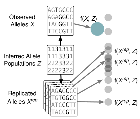
Given observed genotype data, checking admixture models with a PPC works as follows (Figure 1). We first fit an admixture model to the data, estimating ancestral populations and individual-specific population proportions. Note that most analyses end here, e.g., with illustrations of the population proportions as in Figure LABEL:rainbow-diagram. We then simulate genomes from the posterior predictive distribution, using posterior estimates of the latent parameters to draw synthetic genetic data that share the same latent population structure as the observed data; we repeat this process many times to create a collection of replicated data sets. Finally, we evaluate and compare discrepancy functions on both the replicated data sets and the observed data. The discrepancy may be a function of both observed and latent variables [10, 11], and our discrepancies measure important population statistics including within-population genetic variance and background linkage disequilibrium (LD). Specifically, we compare discrepancies computed on the observed data to the empirical distribution of the discrepancies computed on the replicated data. When an observed discrepancy is not likely relative to the replicated discrepancies, the PPC suggests that the model is misspecified (with respect to the discrepancy) for the observed data. We maintain that PPC assessments are best made visually [11, 12].
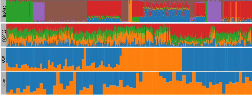
We used PPCs to check for misspecification in four genomic data sets: HapMap phase 3, Europeans, African Americans, and continental Indians. These data have been previously characterized using an admixture model and have qualitatively different types of latent population structure (Figure 2). We developed five discrepancy functions to check for important types of model misspecification in common admixture model analyses. We based these discrepancy functions on common measures in population genetics:
-
•
Identity by state (IBS): we test for the impact of long-range SNP correlations on within-population variance estimates by quantifying the genomic variation among pairs of individuals within alleles from the same ancestral population;
-
•
Background LD: we test for the impact of short-range SNP correlations on population-specific allele frequency estimates by computing the autocorrelation between SNPs, or background LD;
-
•
: we test the appropriate numbers of ancestral populations by computing among labelled and inferred ancestry;
-
•
Assignment uncertainty: we test how distinct the ancestral populations are from one another by quantifying uncertainty in ancestral population assignment;
-
•
Association tests: we test whether or not the inferred population structure adequately controls for confounding latent population structure in association mapping studies by quantifying the difference in statistical significance of corrected associations versus uncorrected associations under the null hypothesis of no association.
As we note in the Discussion, using and comparing PPCs with several discrepancies lets us innovate the model in the directions for which it is most important.
With five discrepancies and four data sets, PPCs reveal that each application of the admixture model meets and diverges from its assumptions differently. Each PPC indicates when we might extend the model to better match the complexities of the study data, and in the Discussion we discuss specific extensions to address each model application for which we find the model is misspecified. While we focus here on the admixture model, we emphasize that assessing the model fitness is important in any application of statistical models to genetic data. PPCs give a framework for visually and quantitatively understanding how and when inferred latent variables cannot be safely interpreted or are unreliable for use in downstream analysis.
2 Results
We used PPCs to assess the fit of an admixture model to data from four genomic studies. We developed five discrepancy functions, each of which measures the degree to which the fitted model captures one aspect of the data. These discrepancies are functions of data and latent structure, and are based on common statistics in population genetics that are important to capture when using or interpreting inferred latent variables. They are (i) inter-individual similarity (ii) linkage disequilibrium within genomes (iii) similarity between inferred ancestral populations and reported geographic labels (iv) distances between ancestral populations and (v) use of model parameters to control for latent population structure in downstream association studies. Here we report our findings.
We first describe the admixture model and outline our procedure for using a PPC to check for misspecification. The admixture model uses allele frequencies across genomes to recover individual-specific ancestry proportions and population-specific allele frequencies. The observed data include individuals, each with single nucleotide polymorphisms (SNPs). Each SNP for individual is represented as two binary variables, , where is the number of copies of the minor (less frequent) allele (genetic variant). The admixture model assumes that there are ancestral populations that describe these data, where is specified a priori, and that each population is associated with location-specific allele frequencies . It assumes that individual ’s genotype data are generated as follows: a) draw individual-specific ancestry proportions from a uniform Dirichlet distribution (i.e., parameter ); b) for each SNP , draw two categorical variables and from a multinomial distribution with parameter ; these latent variables indicate the ancestral populations assigned to the two copies of that SNP; c) conditioned on the assigned ancestral populations, draw two alleles for SNP using the corresponding allele frequencies; that is, draw each from a Bernoulli with parameter .
Conditioned on data, the admixture model estimates the posterior distribution of the latent population structure. This structure is encoded in the ancestral population proportions (illustrated in Figure 2), the population-specific allele frequencies , and the assigned ancestral populations . A sampling approach for estimating this posterior is implemented in the structure software [6]; here we use expectation maximization (EM). See Methods for the complete admixture model specification and a description of our method for parameter estimation.
Interpreting and using the posterior probabilities of ancestral proportions assumes that the model is a good fit to the data; the PPCs we developed check this fit. For each observed genomic data set (and number of populations ), we first estimated the latent parameters: , , and . With these estimates, we generated a collection of replicated genotype data sets. For each one, we drew SNPs for the same individuals, holding the latent population structure and fixed. This results in a set of simulated individuals . In particular, for all and , we drew and similarly for . Note that the replicated data were generated conditional on the inferred latent variables; we do not need to re-estimate them at any point in our analysis. For each data set and fitted admixture model we generated 100 replicated data sets (see Methods).
For each PPC, we developed a discrepancy function , which is a function of the data and latent structure. In our PPCs, each discrepancy function partitions the alleles by assigned ancestral population and produces scalar values. We computed the observed discrepancy and the replicated discrepancy for each replicated data set. The empirical distribution of is an estimate of the posterior predictive distribution of the discrepancy. Thus we checked model fitness by locating the observed discrepancy in this distribution. If we found that the observed discrepancy was an outlier with respect to this estimate of the posterior predictive distribution, then we concluded that the model is not a good fit to our data with respect to the discrepancy.
For each PPC, we used statistical visualizations and assessments of significance to summarize the results [18]. The PPC plots visualize the observed discrepancy against its posterior predictive distribution; model misspecification is indicated by observed discrepancies that appear to be outliers. We plotted the value of the replicated discrepancies with grey circles and the observed discrepancy with a offset solid circle. We colored the observed discrepancy to code its -score, the number of standard deviations from the mean of the replicated discrepancy. Finally, we calculated the likelihood ratio that the -scores were jointly generated from a standard normal distribution. The number of grey stars at the top of each figure corresponds to the level of deviation from standard normal (see Methods), and these stars quantifies the magnitude of model misspecification with respect to a discrepancy.
Our results include evaluations of four genomic studies (see Methods for preprocessing details). For simplicity, we set the number of ancestral populations from the research literature. (We extend the results to many in Supplemental Information.) We study the following data sets:
-
•
The HapMap phase 3 (HapMap) data include individuals genotyped at SNPs from a number of populations worldwide; we expect these individuals will come from distinct (and, in a few cases, admixtures of distinct) ancestral populations [19]. Each individual is labeled with the location of the sample collection. Following prior work, we set [20].
-
•
The POPRes (POPRES) data include individuals genotyped at SNPs from a continental Europe [15, 21]. We expect the ancestry of these individuals to be an admixture of populations defined on a continuous geographic gradient instead of distinct ancestral populations [14]. Each individual has a label describing the geographic birthplace of their grandparents, and we included individuals only if all four grandparents shared the same birthplace. Following prior work, we set [14].
-
•
The African American (ASW) data include African American individuals from the Southwest US, individuals from Utah of Northern and Western European ancestry (CEU), and Yoruba individuals from Ibadan, Nigeria (YRI) included in the 1000 Genomes Project genotyped and sequenced at SNPs [16]. We expect the ancestry of the genotypes from the ASW individuals are admixed from two distinct and distant ancestral populations: European and Yoruban (West African). Individuals are labeled as ASW, CEU or YRI. We set because all individuals are thought to have ancestry from only European and Yoruban populations.
-
•
The Indian data (Indian) include individuals genotyped at SNPs from tribal groups across India [17]. The ancestry of each of these individuals’ genotypes is admixed between two distinct but closely related ancestral groups: North Ancestral Indian and South Ancestral Indian, and there are tribal labels associated with each sample. Following prior work, we set [17].
We number and describe the estimated ancestral populations in Table 1; see also Figure 2. We are using a fixed number of ancestral populations for each study, and we keep this numbering consistent throughout the figures presented in the Results.
Below, we describe each discrepancy and how each study fared under its lens. Then, we shift the focus to the genomic studies, summarizing how well the model fits the data across the collection of discrepancies.
| HapMap | |
|---|---|
| 1 | Pakistan (0.6); N Europe (0.2); Russia (0.2); Israel (0.2) |
| 2 | New Guinea (1.0); S Europe (0.2) |
| 3 | S Africa (1.0); C Africa (1.0); N Africa (0.3) |
| 4 | N Europe (0.7); Israel (0.7); N Africa (0.7); S Europe (0.7) |
| 5 | S America (1.0); C America (0.9) |
| 6 | Japan (0.9); China (0.9); SE Asia (0.8); Russia (0.3) |
| POPRES | |
| 1 | Ukraine (0.5); Slovenia (0.5); Croatia (0.4); Bosn. Herz. (0.4) |
| 2 | Norway (0.6); Latvia (0.5); Finland (0.5); Denmark (0.5) |
| 3 | Portugal (0.3); Spain (0.3); Bulgaria (0.3); Switz. (0.3) |
| 4 | Slovakia (0.6); Turkey (0.6); Greece (0.5); Italy (0.5) |
| ASW | |
| 1 | YRI (1.0); ASW (0.8) |
| 2 | CEU (1.0); ASW (0.2) |
| Indian | |
| 1 | Kurumba (0.8); Bhil (0.8); Tharu (0.7); Vaish (0.7) |
| 2 | Vysya (1.0); Velama (0.8); Srivastava (0.8); Kamsali (0.7) |
2.1 Discrepancy in within-population genomic variation
Population admixture models are often used to explain similarities between individuals’ genotypes: if two individuals have portions of their chromosomes that are descended from the same ancestral population, they will, probabilistically, have more alleles in common than two individuals descended from distinct ancestral populations according to the admixture model. How many more alleles these individuals have in common depends on the separation between ancestral populations, the proportion of the genomes with shared ancestry, and within-population genetic variation.
We developed a discrepancy function to compute the identity by state (IBS) between pairs of individuals, which measures conditional similarity of alleles in unrelated individuals [22]. For a pair of individuals, we averaged the number of alleles in common across the genome for SNPs that share the same ancestry assignment in the fitted model [23]. For this discrepancy function, a pair of individuals with a discrepancy of for population indicates that of the alleles assigned to population in both individuals are identical and indicates different alleles. A misspecified model with respect to a discrepancy function measuring within-population variation may imply that we cannot safely ignore admixture LD, or (possibly long distance) genetic correlations induced by recent admixture of distinct populations, in our admixture model [24].
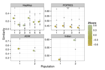
We performed the PPC and found that HapMap, ASW, and Indian results show that the within-population variation is well captured by the admixture model (Figure 3). In contrast, the POPRES data show consistently underestimated average inter-individual similarity, which indicates model misspecification for this discrepancy. Note that the two studies with distinct, well-separated populations (HapMap, ASW) tended to have -scores greater than zero indicating greater than expected inter-individual similarity on the observed data; the two studies with less well-separated populations (POPRES, Indian) have -scores below zero, indicating less similarity than expected.
We also looked at the observed discrepancy without the context of the replicated discrepancy. In the POPRES data and, to a lesser degree, the Indian data, the average similarity of individuals is constant between ancestral populations. This might be expected when modeling data with continuous ancestral population structure. In contrast, the HapMap data and, to a lesser extent, the ASW data exhibit more variability across ancestral populations. This may be a function of variable heterozygosity within the distinct ancestral populations [25]. The higher observed discrepancy in ASW relative to the parallel recovered ancestral populations in the HapMap data may suggest that, within this population of individuals with African and European ancestry, there is less variability within the ancestral populations than in estimates of these populations from non-admixed individuals (European and Yoruban HapMap individuals, for example). This is interesting in light of recent estimates of the effective population size of the ASW population, which is an order of magnitude greater than either the European or Yoruban effective population sizes [26].
A mismatch in observed and replication inter-individual similarity leading to a failure of this PPC may be due to admixture linkage disequilibrium (LD). Admixture LD arises because ancestral recombination events will induce haplotype blocks, or stretches of the haploid chromosome, that are shared among many individuals in a population [27, 28]. Haplotype blocks are population specific: the recombination hotspots, the strength of correlation within the blocks, and the block length will be specific to each population based on its recombination history. A few population specific features, including expansion rate and migration rates, influence these haplotype block characteristics [29]. As noted in earlier work (e.g., [30]), Haplotype blocks, and resulting admixture LD, may account for greater than expected similarity among individuals within these studies. Lower than expected similarity is likely due to the proximity of the ancestral populations: if the ancestral populations are difficult to distinguish with respect to allele frequencies, then SNP-specific ancestral assignments will be arbitrary, and within-population allele variance will be higher in the observed data than is captured by the Bernoulli model and found in the replicated data.
2.2 Discrepancy in background LD
Linkage disequilibrium (LD) is the non-random assortment of alleles across the genome. LD occurs when alleles are not inherited independently: the alleles at one genomic locus provide information about the alleles at another locus. The process of recombination in diploid chromosomes implies that alleles that are nearby on a chromosome are inherited together unless a recombination event occurs, creating dependencies in local genotypes population-wide. Recombination is an infrequent event across a genome: for a single offspring, there are on average a small number of recombination events per chromosome, with high variance [31]. Recombination events within a population lead to a block-like correlation structure of genotypes across the genome, where polymorphisms adjacent in the chromosome will be well correlated (referred to as background LD, in contrast to possibly long-distance dependencies induced by admixture LD). This correlation decays as the chromosomal distance increases (although not uniformly). Although each study we analyzed contains local correlation patterns, the admixture model assumes independence of every SNP conditional on population ancestry.
We assessed the fitted admixture model for local correlation structure among SNPs. To do this, we built a discrepancy function (LD discrepancy) that measures local dependencies among SNPs using mutual information. Although we chose mutual information, the history of statistics to quantify background LD is rich [32], and there are other possibilities for this discrepancy statistic. Mutual information (MI) measures the dependence between two random variables, here, the observed alleles at two loci, and . Specifically, MI quantifies the the reduction in uncertainty about random variable given knowledge of the state of (or vice versa; MI is symmetric) for a pair of discrete random variables [33] (Eqn. 1). If two SNPs are independent (i.e., in linkage equilibrium, or inherited independently), MI will, theoretically, be zero. However, finite samples imply that, even when two SNPs are in linkage equilibrium, the MI may be greater than zero by chance. Our discrepancy uses MI to measure dependence between adjacent pairs of assayed SNPs. We measure the average MI between all pairs of genotypes assigned to the same population. We checked lags between pairs of SNPs varying between and , indicating up to intervening SNPs between the pairs of tested SNPs along the chromosome.
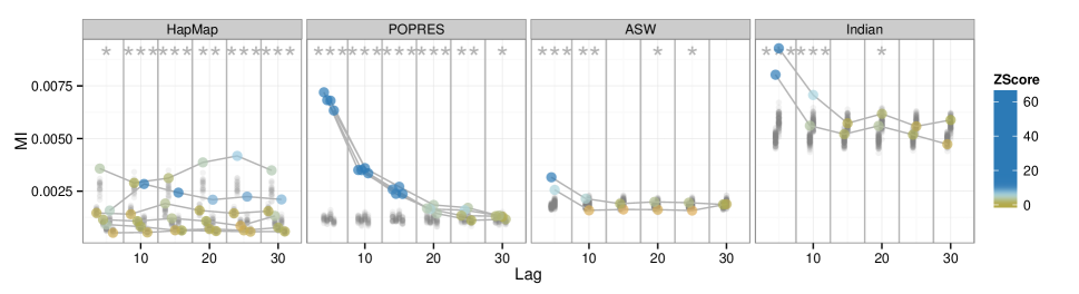
When we applied this LD PPC to our data, we found that, across studies, the models were generally misspecified at small lags (Figure 4). For all studies but HapMap, the -scores show that, as the lag grows, the MI values on the observed data tend toward underestimates of MI in the posterior predictive distribution. The -scores for the POPRES data deviate substantially from a standard normal for all lags indicating more observed background LD than expected. The model’s independence assumption across SNPs manifests in replicated values that have near identical distributions across lags. Failure of this PPC may raise the possibility of using a subset of SNPs with low pairwise LD; however, admixture models rely on greater SNP densities to enable the separation of similar ancestral populations. Below we describe model extensions to address failure of the LD PPC.
We also looked at the observed discrepancies alone. In POPRES and Indian data, we saw that background LD decays rapidly with observed SNP lag on average [34]. In the POPRES data, we found the measurements of background LD to be consistent across inferred populations (Figure 4). In the HapMap data, background LD differs among distinct populations [35]; this is expected because LD is impacted by population-specific effects, including migration, deviations from random mating, and selection [36]. In HapMap and, less so, the ASW data, background LD is fairly uniform across different lags. It is possible that this difference may be a function of the density of SNPs and SNP ascertainment biases, which differs across studies and genotyping methods, but we found that these results persist for lags up to 1000 adjacent SNPs. Note also that the HapMap data include almost 2.5 times more SNPs than the POPRES data.
2.3 Discrepancy in reported ancestry
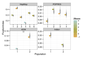
In admixture models, it is often assumed that self-reported ancestries provide no additional information above individual-specific ancestry parameters. We tested misspecification with respect to this assumption. We developed a PPC for inferred population-specific values of the fixation index as compared to self-reported ancestry or geography labels. measures the degree to which the variance of allele frequencies within reported ancestries differs from the variance of those alleles in the study conditioned on inferred population assignment. Using the fitted admixture model to partition alleles into one of inferred ancestral populations, measures whether or not subdividing these alleles by individual-specific reported ancestry reduces the variance of those allele frequencies. The is zero if no additional population structure exists in the reported ancestries beyond what is already recovered in the inferred ancestral populations. Conversely, large values of indicate that the reported ancestries capture additional structure—quantified by reduced allele variation within individuals sharing reported ancestry—not found in the estimated populations. For a fitted admixture model with populations, we evaluated this population-specific discrepancy function by computing values, one for each inferred ancestral population, with respect to reported ancestry (Eqn. 2).
We computed the PPC for the discrepancy, and we found that, except in ASW, the estimated genetic ancestry often reflects all of the population structure in the reported ancestry (Figure 5). If we perform this PPC over many different values of ancestral populations , we found that this PPC tends to fail for values of that are inadequate to explain variation in the observed data (Figure S3). This discrepancy appears to be, in these four studies, an effective approach to evaluate the range of well-specified numbers of ancestral populations in the admixture model. Based on previous observations, we hypothesize that LD is inducing a phantom population in the ASW study that is not captured using two ancestral populations [37]. This would lead to the failure of this PPC, although the reference individuals included are thought to capture the two admixed ancestral populations of the ASW individuals[16].
Note that the observed varied considerably across studies (Figure 5). As with other discrepancy functions, HapMap and ASW show greater variability of observed values across populations than POPRES and Indian due to greater heterogeneity of ancestral populations. The two ASW populations have consistently lower observed values, possibly suggesting that the fitted admixture model captures most of the information in the reported ancestries (ASW, CEU, and YRI). Indeed, is undefined for several populations within the ASW models because all the alleles assigned to those populations were from individuals with a single reported ancestry. In the context of the replicated data, however, this conclusion is shown to be incorrect: there is latent structure in the data that is not captured well by two ancestral populations. The Indian data, with distinct reported ancestries, have higher overall values: individuals within each reported ancestry have a range of admixture between Ancestral North Indian and Ancestral South Indian [17], and reported geographic labels are, unsurprisingly, a poor indicator of admixture proportions across these individuals.
2.4 Discrepancy in uncertainty in ancestral population assignments
We chose these four studies because they represent distinct patterns of admixture (Figure 2): in the HapMap data, most individuals have a majority of genomic ancestry explained by one or two populations; in POPRES, although regional variation in ancestry proportions is evident, most individuals have substantial ancestry contributions from all four populations. We measured the degree of uncertainty of individual-specific population assignments to determine whether this uncertainty is characteristic of the model parameters or evidence of model misspecification.
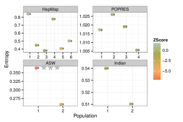
The discrepancy function for this task quantifies the average entropy, or uncertainty, of the ancestral population assignment for alleles in the fitted model. We used the fitted admixture model to compute estimates of the conditional probability of the assignment of each SNP allele to each ancestral population . We then computed, for each population, the average entropy of this conditional probability across individuals and SNPs, including SNPs assigned to the same population (Eqn. 3).
We performed PPCs with this entropy discrepancy, and found that this model is grossly misspecified for the ASW study with respect to uncertainty in allele-specific ancestry assignments (Figure 6); the remaining three studies did not indicate problems with this PPC. This result is interesting considering the low variation in average entropy among the replicated data; indeed, the replicated points appear near-identical at the scale of the visualization. As with the PPC, we hypothesize that the failure of this PPC on the ASW population may be due to the additional ancestral structure induced by LD that is not captured well with two ancestral populations.
The success of this PPC across three studies is also unexpected when considering the observed discrepancies alone. We found that the POPRES and Indian studies showed high observed average entropy relative to the other studies along with low variation in observed average entropy across populations, indicating a high degree of uncertainty in population assignments (Figure 6). This uncertainty does not appear to be caused by lack of convergence in the parameter estimates: this same behavior is observed for models fit with ten times as many EM iterations. In contrast, the HapMap and ASW studies, which have distinct ancestral populations, have greater variance of average entropy across populations within , indicating greater uncertainty in some population assignments relative to others.
2.5 Discrepancy in correcting for population structure in genome-wide association studies
A final discrepancy function we considered is the value of using estimates of individual specific admixture proportions to correct for population structure in association studies [1, 2, 38, 39, 40]. Association mapping uncovers associations between genetic variants (e.g., SNPs) and traits (e.g., height, disease status, cholesterol levels). It is well-appreciated that correcting for population structure in association mapping is essential because latent structure leads to false positive associations when alleles that have different frequencies across populations are mapped to traits with differential rates across populations [41, 42]. We note that, in the original manuscript describing the use of admixture model parameters to correct for population stratification in association studies [1], they effectively performed the same PPC as we applied here without describing it as a posterior predictive check.
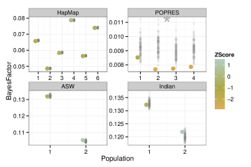
For this task, we evaluated the effect of the fitted admixture parameters on the distribution of Bayes factors (BFs) comparing the null hypothesis of no association between a SNP and the trait controlling for population assignment, and the alternative hypothesis of an association between a SNP and the trait, controlling for population assignment (following prior work [1]; see Methods). We randomly generated binary traits for each study using a population in the generative model, creating phenotypes with different rates within our estimated populations but with no explicit association with any SNP. Thus, controlling for population structure, any significant association will be a false positive. The value of the discrepancy for a specific population is computed as the maximum BF over all SNPs. We then computed the -score of the BFs of the observed data associations with respect to the BFs from the replicated data.
We performed this mapping PPC and found that the observed maximum BFs are generally within the expected range when sampling alleles from the fitted model, which provides additional confidence in our ability to reject false positives (Figure 7). The variation in the POPRES replicates highlights why the PPC fails: controlling for fine levels of population structure with noisy discrete estimates is not effective control for structure. It is counterintuitive, though, that the four populations in POPRES have lower than expected observed correction BFs.
The observed discrepancies alone were also informative We found that the maximum BF across studies was small () indicating that this approach to correcting for population structure is broadly effective at avoiding false positive associations. As in previous discrepancies, the variability in maximum BF between populations was greater for HapMap and ASW data than POPRES and Indian data, reflecting greater distinction between populations in the first two studies. The maximum BFs for POPRES are smaller than the other studies, reflecting less significance in tests for association between SNPs and populations; this is not surprising given the homogeneity of the inferred populations and the corresponding randomly generated phenotypes.
2.6 Summarizing PPC results within study
We turn our attention to summarizing the results from the five PPCs for each of our genomic studies. Our results across PPCs tell a complex story for each study that indicates specific misspecified assumptions.
HapMap phase 3.
Across our application of PPCs to the HapMap phase 3 data, we found that the background LD discrepancy PPC indicated a gross model misspecification, highlighting the negative impact of the assumption of independent SNPs. Other PPCs did not find misspecification with on these data. Two ways to address this model misspecification with respect to background LD in these well-separated ancestral populations would be to a) prune the SNP data drastically to select a near-independent set of SNPs from which ancestry may be estimated, or b) model background LD explicitly (see Discussion).
European samples.
Across our application of PPCs to the POPRES data, we found that the admixture model with ancestral populations generally indicated similar variation in discrepancy within and across populations. Many of the failures of the PPCs on these data could be used together to highlight model misspecificiation, as the continuous structure of the ancestral populations is not captured well by the discrete populations assumed by an admixture model. A possible solution is to model latent structure for these data with a continuous population model (e.g., principal components-based [43, 44]).
African Americans.
PPCs on the ASW data with showed that the ancestral population corresponding to European ancestry was well captured in the observed data with respect to the replicated data, but the population corresponding to Yoruban ancestry was often misspecified for the observed data with respect to the replicated data; the PPC and the entropy PPC show this differential fit. For these data, explicitly modeling admixture LD may enable a better fit with two ancestral populations, eliminating the need to use an additional ancestral population to control for the effects of long distance haplotype block correlations [37].
Continental Indians.
With PPCs on the Indian data with , we found that the failure of the average entropy PPC indicates that the underlying estimates of the two ancestral populations have substantial uncertainty. Relying on these estimates to characterize ancestral population allele frequencies or determine admixture proportions for each individual is unjustifiable. These data may also benefit from using a continuous model of ancestral populations because of the difficulty of differentiating these two fairly proximal ancestral populations many generations after the admixture events [17].
3 Discussion
We have developed posterior predictive checks (PPCs) for analyzing genomic data sets with the admixture model. We have demonstrated that the PPC—estimating the posterior predictive distribution and checking the likelihood of the true observed data under this distribution—gives a valuable perspective on genetic data beyond statistical inference of model parameters. In the research literature, fitted admixture models are often accompanied by a ‘just so’ story to explain the inferred parameters and how they are reflective of ancestral truth [13]. The model may suggest these hypotheses, but only conditioned on the model being a good fit for the observed data. PPCs check this assumption of good fit, giving weight to the hypotheses by confirming that the underlying assumptions do not oversimplify the existing structure in the observed data. In this paper, we developed PPCs for the admixture model, designing biological discrepancy functions to quantify the effect of the model assumptions on interpreting and using the estimated parameters for downstream analyses.
Statistical modeling of genetic data requires us to balance the complexity of the model with its capacity to capture the data at hand. As examples of limitations, we may not have enough data to support an overly complex model, or the model class that that we want to fit may be too complex given our computational constraints. Thus, we support the iterative practice of fitting the simplest model (i.e., the one we fit here), checking whether a higher resolution model is needed, and then improving the model only in the ways that result in more reliable interpretations of the results. PPCs can drive this process of targeted model development, pointing us towards enriched Bayesian admixture models along gradients that quantifiably improve their performance for the exploratory tasks that matter. With this practice in mind, we revisit the PPCs described above and discuss how we might enrich the simple admixture model to address its misspecified assumptions.
Many population studies have applied admixture models to explore and quantify genetic variation between individuals within and across ancestral populations [13, 45, 46]; these analyses may benefit from the inter-individual PPC. For studies where this PPC indicates misfit, prior work has adapted the admixture model to control admixture LD by explicitly modeling haplotype blocks for each ancestral population instead of modeling each SNP separately [30]. In particular, the SNP-specific ancestry assignment variables for each individual are modeled by a Markov chain, where the probability of transitioning to a different ancestral population from one position to the next has an exponential distribution. This specifies a Poisson process describing the length of haplotype blocks across the chromosome, with global rate parameter .
Many studies have noted that background LD may lead to phantom ancestral populations [37]; applying admixture models to genomic data that contain background LD may find the SNP autocorrelation PPC useful. After identifying model misspecification using our background LD discrepancy function, we could extend the admixture model to explicitly capture background LD. Above we described a Markov model on the variables. It assumes that, conditional on ancestral population assignment, genotypes are independent. Extending this idea, SABER [47] implements a Markov hidden Markov (MHMM) model to capture both haplotype blocks and background LD by adding a Markov chain across the population-specific allele frequencies in . Others have further extended this model in various ways, including estimating recombination events explicitly in the MHMM [48].
The discrepancy function effectively checks for a misspecified number of ancestral populations . The ubiquitous problem of selecting a number of ancestral populations is, arguably, the most substantial hurdle to overcome in applying admixture models, or latent factor models generally, to data [6, 13, 2]. Methods and statistics have been proposed to evaluate the proper number of latent ancestral populations, often motivated by [6, 49]; additionally, nonparametric Bayesian models estimate the posterior probability for each [50, 51]. We propose a PPC with the discrepancy for general use in evaluating appropriate ranges of the number of ancestral populations for a specific study. A simple adaptation of the model to correct for a failure of this PPC is to change the number of ancestral populations (Figure S3).
There are also explicit model adaptations that will affect the of the inferred ancestral populations. For example, one can build hierarchical models that allow the sharing of allele frequencies across populations for some SNPs; this was implemented in the structure 2.0 model, which includes a hierarchical component to allow similar allele frequencies across ancestral populations (the so-called model) [30]. A second example is from the topic model literature (similar models applied to modeling text documents), where the ancestral populations are captured in a tree-structured hierarchy [52, 53]. In the corresponding admixture models, the root node would include SNPs that have shared allele frequencies across all ancestral populations; at the leaves, the population-specific allele frequencies would include SNPs that have a frequency in that population that is different than the frequency in all other ancestral populations (referred to as ancestry informative markers [20]).
Previous population studies have explored and interpreted the population-specific SNP frequencies estimated by admixture models [54, 55, 56]; almost all applications of this admixture model have used MAP estimates of ancestry assignments to determine the proportion of admixture in individuals [20, 14]. The average entropy PPC will check model misspecification for ancestry assignment, and has implications for interpreting estimates of SNP frequencies. To adapt the model to this misspecification, the hyperparameters for the Dirichlet-distributed allele-specific ancestry assignments may be changed. (We and others set to [6], giving equal weight to all possible contribution across ancestries for each SNP.) In particular, we might give higher weight to admixture proportions near and by setting for studies where we expect low levels of admixture (e.g., the HapMap data). The equivalent change for the hyperparameters in the population-specific allele frequency parameters would encourage for allele frequency spectrums that more closely match what we find in natural populations [57]. Another relevant model adaptation would be to modify the distribution of a SNP to be not Bernoulli but instead Poisson [58], normal [59], or something more sophisticated [60, 61]. We emphasize that, though these extensions seem reasonable, the PPC with this discrepancy found little need to modify the admixture model assumptions in our current studies. The exception to this point is the ASW study, although we hypothesize that correcting for background LD as suggested above will address this misspecification.
We believe that all model-based methods to control for population stratification in association mapping will benefit from application of the mapping PPC, including linear mixed models and non-generative methods such as EIGENSTRAT [2, 62]. Failure of the association mapping PPC indicates that the estimates of population structure are insufficient to correct for the confounding latent structure in the individuals. There are many directions to consider for mitigating this type of model misspecification. As examples, one may use larger numbers of estimated principal components or ancestral populations, use alternative approaches to specifying the latent structure variables, or correct for structure that are estimated on local regions of the genome. This same discrepancy function—replacing with the estimated random effect from linear mixed models—would be useful in quantifying model misspecification for these alternative methods for association mapping in the presence of confounding population structure [63, 64, 65].
Applied statisticians develop models to capture the biological complexity of their data. To form hypotheses from these models, however, we need assurances that the data can support them. PPCs provide a simple mechanism to quantify when a model is sufficient or when it needs additional structure to support downstream analysis. While we have focused on the admixture model, the PPC methodology applies to any probabilistic model of data. For example, we believe there could be a substantial role for PPCs in evaluating demographic models. As we continue to collect complex genomic data, we continue to develop complex models to explain them. Equally important to building our repertoire of statistical models for analyzing genomic data is to build our repertoire of ways to check those analyses.
3.1 Genomic study data
We downloaded the HapMap phase 3 release #3 genotype data from the NCBI website [19]. We downloaded the POPRES data from dbGaP (accession number phs000145) and filtered these genotype data as described in prior work [21, 14]. We downloaded the ASW genotype data from 61 individuals, CEU individuals, and YRI individuals from the 1000 Genomes Project Phase 1 [16] from the 1000 Genomes FTP server 111ftp://ftp.1000genomes.ebi.ac.uk/vol1/ftp/phase1/analysis_results and pruned these data by randomly sampling 1% of SNPs with MAF . We downloaded the Indian data from the Reich Lab FTP server [17] and processed it as in previous work [14].
3.2 Admixture model and parameter estimation
We used a standard admixture model in this work, as implemented in the Structure software [6], although we built our own software to fit this model to large scale data as described below. We represented ancestral population with a Dirichlet-distributed random variable , for each single nucleotide polymorphism (SNP) , over all possible alleles; we assumed exactly two alleles for each SNP, so this simplified to a beta distribution. We represented individual-specific ancestry proportions for individual as a Dirichlet-distributed variable over populations. To generate a diploid genotype from this model, for each SNP we sampled two multinomial variables with parameter , and , one for each allele copy. We then sampled alleles and from the distributions and , respectively. The generative model has the following form:
where represents the two allele copies. For simplicity, we set and , indicating a uniform prior on the ancestry proportions for each individual and the site-specific allele frequencies for each population [66]. The likelihood for this model has the form:
Without loss of generality, we represent a heterozygous SNP (encoded as a 1) in the data as and , where and are the two alleles at that site [6].
We estimated these parameters and latent variables with an expectation maximization (EM) algorithm that alternates between i) (E-step) estimating the posterior mode for population assignments of individual alleles given estimates for and , and ii) (M-step) maximizing the individual- and population-level parameters given those posterior modes of [67, 66]. The update equations for the E-step, estimating the posterior mode for population assignment for an allele, are
The update equations for the M-step, estimating the model parameters for individuals and SNPs given the posterior mode for , are:
We initialized the population-specific minor allele frequency parameters to the empirical proportion of the minor allele in the training data, plus a uniform random variable , truncating extreme values so that . To initialize population proportions for each individual, we drew uniform random variables and set . We iterated between these E- and M-steps for 1000 iterations. We also ran a number of models to 10,000 iterations, but found no substantial differences in the fitted models, supporting convergence of the parameter estimates in 1000 iterations.
3.3 Discrepancy: Inter-individual similarity for IBD
We measured similarity between individuals (identity by descent) with respect to population by counting the number of alleles that are shared between individuals with population assignment (i.e., the Manhattan distance) and dividing by the total number of alleles with population assignment [23]. The value of the discrepancy function is the average proportion of shared alleles over all pairs of individuals. We ignored pairs of genomes that shared fewer than alleles assigned to a population .
3.4 Discrepancy: Mutual information for background LD
We calculated population-specific MI for each pair of adjacent SNPs within a lag of all integers . This window is with respect to the ordering of the SNPs in our filtered data set based on chromosomal position, although the actual distance in base pairs between SNPs varies dramatically across studies and SNP pairs. As with the inter-individual similarity, we only compared pairs of SNPs if they shared population assignments.
This discrepancy function calculates mutual information (MI) quantified in bits between the observed alleles at two adjacent loci separated by SNPs, and . For haploid genotypes, both generated from the same ancestral population , we computed:
| (1) | |||||
As calculating this statistic is computationally intensive, we computed MI for this SNP window only over the first 10,000 SNPs in each study.
3.5 Discrepancy: Distance between estimated ancestral populations and geographic labels
We computed the statistic on alleles assigned to one ancestral population relative to the geographic labels using Wright’s estimator of , which considers single alleles at each genomic locus [68]. In our data, each individual has exactly one geographic label , but the individual’s alleles are assigned to possibly many ancestral populations. The probability of an allele for SNP and population is computed as , where is the total number of alleles assigned to population and is an indicator function. We further partition these population-specific probabilities by geographic label : , where is the total number of alleles assigned to population for individuals with geographic label , which may be zero, in which case this probability is set to zero. With these probabilities in hand, and assuming Bernoulli distribution of alleles (so that the variance of these distributions is estimated from the expectations), we calculate fixation index as
| (2) |
where is the total number of geographic regions with non-zero allele counts for population .
3.6 Discrepancy: Average entropy
We computed the average entropy discrepancy function as the average entropy for each estimated ancestral population over all alleles assigned to a population. Given estimates of the distribution of ancestral populations for an individual , , and the probability of the minor allele for a SNP across populations, , we calculated the posterior probability of each population for the observed alleles in that individual’s genome. The entropy is
| (3) |
Then we computed the discrepancy as the average entropy for each ancestral population over all alleles assigned to a population.
3.7 Discrepancy: Correcting latent structure in association mapping
For each model and each ancestral population , we generated a binary phenotype vector of length , simulating a condition that is associated with that population. In particular, for the phenotype vector, we sampled a Bernoulli random variable for each individual with probability , so individuals with ancestry in population are more likely to exhibit the phenotype. To compute the discrepancy function for the GWAS association controlling for ancestry, we computed, for each SNP, the Bayes factor (BF) for each SNP as the ratio of the likelihood of the genotype given the phenotype and the population assignment of the SNP (), and the likelihood of the genotype given the population assignment () [1, 69]. We used a beta-binomial model with symmetric smoothing parameter for the generalized linear model of association. The value of the discrepancy for a population is the maximum BF over all SNPs. For each population , we sampled random phenotypes ten times using that population as the risk factor and averaged the result of the discrepancy function over these ten samples.
3.7.1 Diploid data
Diploid data complicates some discrepancy functions, because, conditionally, each of the two copies of an allele may be generated from (or, equivalently, assigned to) different ancestral populations. As in the original specification of the admixture model, we divided single ternary observations into the sum of two binary observations . Each binary observation has a separate latent population assignment . Two of our discrepancy functions (i.e., inter-individual similarity, MI) compared pairs of SNPs and were modified to account for as many as two population assignments per SNP.
Let be the first and second hidden assignment variables at SNPs and , and be the observed alleles associated with those hidden variables. There are four possible comparison scenarios, depending on how many of the latent population assignment variables are set to among these two SNPs.
-
1.
No Match. If at least one of the positions has no hidden variables equal to , there are no relevant comparisons.
-
2.
Single Match. If exactly one hidden variable at both positions is equal to , the two observations associated with those matching variables are comparable. For example, if and , but and are set to two other populations, then we compare with .
-
3.
Single-Double Match. If one location has one latent assignment variable equal to , and the other location has both latent assignment variables equal to , there are two possible comparisons. For example, if and , we compare with and with .
-
4.
Double-Double Match. In the case where all four hidden variables are equal to , we have four possible comparisons: with , with , with , and with .
3.8 Posterior predictive checks
We generated replications of the observed data by sampling from the fitted model distributions:
| (4) |
For a discrepancy function of alleles and their population assignment variables, , we calculated , holding the latent variables fixed. For each of our PPCs, we set , except for the intra-individual similarity that considers all pairs of replicates, where we used . We calculated the mean and standard deviation of the values of the discrepancy function over all replications for each of ancestral population. We then computed an empirical -score to compare the function values for the observed data to the mean and standard deviation of the function values for the replications: . Given these population-specific -scores, we estimated the significance of their deviation from a standard normal distribution by computing a Bayes factor (BF) as the ratio of density of the -scores under a the normal distribution with MLE parameters over the likelihood of the -scores under the standard normal. We report this BF in all figures – three stars for , two stars for , and one star for – where a larger BF indicates greater distance from the standard normal for these observed -scores.
Acknowledgements
The authors would like to acknowledge the groups that made these data publicly available: HapMap Consortium, Glaxo-Smith Klein, 1000 Genomes Project, and David Reich. BEE was funded through NIH R00 HG006265.
References
- 1. Pritchard JK, Stephens M, Rosenberg NA, Donnelly P (2000) Association mapping in structured populations. American journal of human genetics 67: 170–81.
- 2. Price AL, Patterson NJ, Plenge RM, Weinblatt ME, Shadick NA, et al. (2006) Principal components analysis corrects for stratification in genome-wide association studies. Nature Genetics 38: 904–909.
- 3. Reich D, Patterson N, Kircher M, Del n F, Nandineni MR, et al. (2011) Denisova admixture and the first modern human dispersals into southeast asia and oceania. Am J Hum Gen 89: 1–13.
- 4. Moorjani P, Patterson N, Hirschhorn JN, Keinan A, Hao L, et al. (2011) The history of african gene flow into southern europeans, levantines, and jews. PLOS Genetics .
- 5. Wang S, Lachance J, Tishkoff SA, Hey J, Xing J (2013) Apparent variation in neanderthal admixture among african populations is consistent with gene flow from non-african populations. Genome Biol Evol 5: 2075–2081.
- 6. Pritchard JK, Stephens M, Donnelly P (2000) Inference of population structure using multilocus genotype data. Genetics 155.
- 7. Gilbert KJ, Andrew RL, Bock DG, Franklin MT, Kane NC, et al. (2012) Recommendations for utilizing and reporting population genetic analyses: the reproducibility of genetic clustering using the program structure. Molecular ecology 21: 4925–4930.
- 8. Box GEP (1980) Sampling and Bayes’ inference in scientific modelling and robustness. Journal of the Royal Statistical Society Series A ( …143: 383–430.
- 9. Rubin D (1984) Bayesianly Justifiable and Relevant Frequency Calculations for the Applied Statistician. The Annals of Statistics 12: 1151–1172.
- 10. MENG XL, RUBIN DB (1993) Maximum likelihood estimation via the ECM algorithm: A general framework. Biometrika 80: 267–278.
- 11. Gelman A, Meng X, Stern H (1996) posterior predictive assessment of model fitness via realized discrepancies. Statistica Sinica 6: 733–807.
- 12. Gelman A, Shalizi CR (2013) Philosophy and the practice of Bayesian statistics. The British journal of mathematical and statistical psychology 66: 8–38.
- 13. Rosenberg NA, Pritchard JK, Weber JL, Cann HM, Kidd KK, et al. (2002) Genetic Structure of Human Populations. Science 298: 2381–2385.
- 14. Engelhardt BE, Stephens M (2010) Analysis of Population Structure: A Unifying Framework and Novel Methods Based on Sparse Factor Analysis. PLoS Genet 6.
- 15. Nelson MR, Bryc K, King KS, Indap A, Boyko AR, et al. (2008) The Population Reference Sample, POPRES: A Resource for Population, Disease, and Pharmacological Genetics Research. American Journal of Human Genetics 83: 347–358.
- 16. Durbin RM, Altshuler DL, Abecasis GR, Bentley DR, Chakravarti A, et al. (2010) A map of human genome variation from population-scale sequencing. Nature 467: 1061–1073.
- 17. Reich D, Thangaraj K, Patterson N, Price AL, Singh L (2009) Reconstructing Indian population history. Nature 461: 489–494.
- 18. Gelman A (2004) Exploratory Data Analysis for Complex Models. Journal of Computational and Graphical Statistics 13: 755–779.
- 19. Altshuler DM, Gibbs RA, Peltonen L, Dermitzakis E, Schaffner SF, et al. (2010) Integrating common and rare genetic variation in diverse human populations. Nature 467: 52–8.
- 20. Rosenberg NA, Li LM, Ward R, Pritchard JK (2003) Informativeness of genetic markers for inference of ancestry. American journal of human genetics 73: 1402–22.
- 21. Novembre J, Johnson T, Bryc K, Kutalik Z, Boyko AR, et al. (2008) Genes mirror geography within Europe. Nature 456: 98–101.
- 22. Bishop DT, Williamson JA (1990) The power of identity-by-state methods for linkage analysis. American journal of human genetics 46: 254–65.
- 23. Weir BS, Cockerham CC (1984) Estimating F-Statistics for the Analysis of Population Structure : 1358—-1370.
- 24. Stephens JC, Briscoe D, O’Brien SJ (1994) Mapping by admixture linkage disequilibrium in human populations: limits and guidelines. American journal of human genetics 55: 809–24.
- 25. Conrad DF, Jakobsson M, Coop G, Wen X, Wall JD, et al. (2006) A worldwide survey of haplotype variation and linkage disequilibrium in the human genome. Nature Genetics 38: 1251–1260.
- 26. Excoffier L, Dupanloup I, Huerta-Sánchez E, Sousa VC, Foll M (2013) Robust demographic inference from genomic and SNP data. PLoS genetics 9: e1003905.
- 27. Daly MJ, Rioux JD, Schaffner SF, Hudson TJ, Lander ES (2001) High-resolution haplotype structure in the human genome. Nature genetics 29: 229–32.
- 28. Gabriel SB, Schaffner SF, Nguyen H, Moore JM, Roy J, et al. (2002) The structure of haplotype blocks in the human genome. Science (New York, NY) 296: 2225–9.
- 29. Greenwood TA, Rana BK, Schork NJ (2004) Human Haplotype Block Sizes Are Negatively Correlated With Recombination Rates : 1358–1361.
- 30. Falush D, Stephens M, Pritchard JK (2003) Inference of population structure using multilocus genotype data: linked loci and correlated allele frequencies. Genetics 164: 1567–1587.
- 31. Fledel-Alon A, Leffler EM, Guan Y, Stephens M, Coop G, et al. (2011) Variation in human recombination rates and its genetic determinants. PloS one 6: e20321.
- 32. Slatkin M (2008) Linkage disequilibrium–understanding the evolutionary past and mapping the medical future. Nature reviews Genetics 9: 477–85.
- 33. Cover TM, Thomas JA (1991) Elements of Information Theory (Wiley Series in Telecommunications and Signal Processing). Wiley-Interscience, 576 pp. URL http://www.amazon.com/Elements-Information-Theory-Telecommunications-Processing/dp/0471062596.
- 34. The International HapMap Consortium (2005) A haplotype map of the human genome. Nature 437: 1299–320.
- 35. Shifman S (2003) Linkage disequilibrium patterns of the human genome across populations. Human Molecular Genetics 12: 771–776.
- 36. McEvoy BP, Powell JE, Goddard ME, Visscher PM (2011) Human population dispersal ”Out of Africa” estimated from linkage disequilibrium and allele frequencies of SNPs. Genome research 21: 821–9.
- 37. (2007) Genome-wide association study of 14,000 cases of seven common diseases and 3,000 shared controls. Nature 447: 661–78.
- 38. Hoggart CJ, Parra EJ, Shriver MD, Bonilla C, Kittles RA, et al. (2003) Control of confounding of genetic associations in stratified populations. American journal of human genetics 72: 1492–1504.
- 39. Satten GA, Flanders WD, Yang Q (2001) Accounting for unmeasured population substructure in case-control studies of genetic association using a novel latent-class model. American journal of human genetics 68: 466–77.
- 40. Devlin B, Roeder K (1999) Genomic control for association studies. Biometrics 55: 997–1004.
- 41. Patterson N, Hattangadi N, Lane B, Lohmueller KE, Hafler DA, et al. (2004) Methods for high-density admixture mapping of disease genes. American journal of human genetics 74: 979–1000.
- 42. Marchini J, Cardon LR, Phillips MS, Donnelly P (2004) The effects of human population structure on large genetic association studies. Nature genetics 36: 512–7.
- 43. Patterson N, Price AL, Reich D (2006) Population structure and eigenanalysis. PLOS genetics 2: e190.
- 44. Price AL, Zaitlen NA, Reich D, Patterson N (2010) New approaches to population stratification in genome-wide association studies. Nature reviews Genetics 11: 459–63.
- 45. Jorde LB, Wooding SP (2004) Genetic variation, classification and ’race’. Nature Genetics .
- 46. Serre D, Pääbo S (2004) Evidence for gradients of human genetic diversity within and among continents. Genome research 14: 1679–85.
- 47. Tang H, Coram M, Wang P, Zhu X, Risch N (2006) Reconstructing genetic ancestry blocks in admixed individuals. American journal of human genetics 79: 1–12.
- 48. Sankararaman S, Kimmel G, Halperin E, Jordan MI (2008) On the inference of ancestries in admixed populations. Genome research 18: 668–75.
- 49. Evanno G, Regnaut S, Goudet J (2005) Detecting the number of clusters of individuals using the software STRUCTURE: a simulation study. Molecular ecology 14: 2611–20.
- 50. Huelsenbeck JP, Andolfatto P (2007) Inference of population structure under a Dirichlet process model. Genetics 175: 1787–802.
- 51. Teh YW, Jordan MI, Beal MJ, Blei DM (2003) Hierarchical Dirichlet Processes. Journal of the American Statistical Association 101.
- 52. Blei D, Griffiths T, Jordan M, Tenenbaum J (2003) Hierarchical Topic Models and the Nested Chinese Restaurant Process. NIPS .
- 53. Adams R, Ghahramani Z, Jordan M (2010) Tree-Structured Stick Breaking for Hierarchical Data. NIPS : 1–9.
- 54. Ardlie KG, Lunetta KL, Seielstad M (2002) Testing for population subdivision and association in four case-control studies. American journal of human genetics 71: 304–11.
- 55. Pickrell JK, Pritchard JK (2012) Inference of population splits and mixtures from genome-wide allele frequency data. PLoS genetics 8: e1002967.
- 56. Gautier M, Vitalis R (2013) Inferring population histories using genome-wide allele frequency data. Molecular biology and evolution 30: 654–68.
- 57. Nelson MR, Wegmann D, Ehm MG, Kessner D, St Jean P, et al. (2012) An abundance of rare functional variants in 202 drug target genes sequenced in 14,002 people. Science (New York, NY) 337: 100–4.
-
58.
D LD, Seung HS (1999) Learning the parts of objects by non-negative matrix
factorization.
Nature 401: 788–791.
Key: Lee1999
Annotation: A specific type of generalized factor analysis. Non-negative matrix factorization paper. - 59. Rasmussen CE (2000) The Infinite Gaussian Mixture Model .
- 60. Yang WY, Novembre J, Eskin E, Halperin E (2012) A model-based approach for analysis of spatial structure in genetic data. Nature Genetics 44: 725–731.
- 61. Paisley J, Wang C, Blei DM (2012) The Discrete Infinite Logistic Normal Distribution. Bayesian Analysis 7: 997–1034.
- 62. Kang HM, Sul JH, Service SK, Zaitlen Na, Kong SY, et al. (2010) Variance component model to account for sample structure in genome-wide association studies. Nature genetics 42: 348–54.
- 63. Listgarten J, Lippert C, Kadie CM, Davidson RI, Eskin E, et al. (2012) Improved linear mixed models for genome-wide association studies. Nature methods 9: 525–6.
- 64. Zhou X, Stephens M (2012) Genome-wide efficient mixed-model analysis for association studies. Nature genetics 44: 821–4.
- 65. Runcie DE, Mukherjee S (2013) Dissecting High-Dimensional Phenotypes with Bayesian Sparse Factor Analysis of Genetic Covariance Matrices. Genetics : genetics.113.151217–.
- 66. David H Alexander JN, Lange K (2009) Fast model-based estimation of ancestry in unrelated individuals. Genome Res .
- 67. Dempster A, Laird N, Rubin DB (1977) Maximum likelihood from incomplete data via the EM algorithm. Journal of the Royal Statistical Society, Series B 39: 1–38.
- 68. Wright S (1969) Evolution and the Genetics of Populations, Vol. II. The Theory of Gene Frequencies. University of Chicago Press.
- 69. Stephens M, Balding DJ (2009) Bayesian statistical methods for genetic association studies. Nature reviews Genetics 10: 681–90.