CONSTRAINING PHYSICAL PROPERTIES OF TYPE IIn SUPERNOVAE
THROUGH RISE TIMES AND PEAK LUMINOSITIES

Abstract

We investigate the diversity in the wind density, supernova ejecta energy, and ejecta mass in Type IIn supernovae based on their rise times and peak luminosities. We show that the wind density and supernova ejecta properties can be estimated independently if both the rise time and peak luminosity are observed. The peak luminosity is mostly determined by the supernova properties and the rise time can be used to estimate the wind density. We find that the ejecta energy of Type IIn supernovae needs to vary by factors of $0.2-5$ from the average if their ejecta mass is similar. The diversity in the observed rise times indicates that their wind density varies by factors of $0.2-2$ from the average. We show that Type IIn superluminous supernovae should have not only large wind density but also large ejecta energy and/or small ejecta mass to explain their large luminosities and the rise times at the same time. We also note that the shock breakout does not necessarily occur in the wind even if it is optically thick, except for the case of superluminous supernovae, and we analyze the observational data both with and without assuming that the shock breakout occurs in the dense wind of Type IIn supernovae.

1. Introduction

Type IIn supernovae (SNe IIn) are a class of SNe in which the signatures of the interaction between the SN ejecta and the circumstellar medium are observed (Schlegel, 1990; Filippenko, 1997). The estimated circumstellar density required to explain the observational properties is much higher than that expected from the standard stellar evolution theory (e.g., Langer 2012). It is generally assumed that the high circumstellar density is due to the high mass-loss rates of the SN IIn progenitors. The estimated mass-loss rates are typically higher than $10^{-3}$ $M_{\odot}~{}\mathrm{yr^{-1}}$ (e.g., Kiewe et al. 2012; Taddia et al. 2013; Fransson et al. 2013; Moriya et al. 2014).

SNe IIn are heterogeneous. For example, their peak luminosities spread in more than two orders of magnitudes (e.g., Richardson et al. 2014; Li et al. 2011). The diversities can be caused by many reasons, e.g., the diversities in circumstellar density, SN ejecta mass, and SN ejecta energy. It is important to understand which observational properties are affected by which physical parameters. By disentangling the origins of the observational diversities, we can constrain the physical properties of the progenitor systems and obtain the better understanding of SNe IIn and their progenitors.

In this Letter, we investigate a way to disentangle the information on the wind density, SN ejecta energy, and SN ejecta mass based on the early light curves (LCs) of SNe IIn. We suggest that the wind and SN properties can be constrained independently if both the rise time and the peak luminosity of a SN IIn are observed. By using the observational rise times and peak luminosities of SNe IIn recently reported by Ofek et al. (2014a), we show how diverse the wind and SN properties should be to explain the observational diversities of SNe IIn.

Ofek et al. (2014a) also performed a similar analysis by using their data mainly focusing on the rise times when they reported the observations. However, they did not use the peak luminosities to constrain the SN properties. In addition, they assumed that the shock breakout always occurs in the dense wind in SNe IIn. The shock breakout does not necessarily occur in the wind even if it is optically thick and makes SNe IIn. Here, we also investigate the case in which the shock breakout does not occur in the wind.

2. Diffusion Time and Characteristic Luminosity

We analytically estimate the diffusion time $t_{d}$ and the characteristic luminosity $L_{p}$ of SNe IIn at $t_{d}$ based on the way presented by Chevalier & Irwin (2011).

2.1. Diffusion Time

The diffusion time $t_{d}$ is estimated as $t_{d}=\tau_{\mathrm{w}}\Delta R/c$, where $c$ is the speed of light, $\tau_{\mathrm{w}}$ is the Thomson scattering optical depth of the wind from the radius $R_{b}$ where photons start to be emitted in the wind, $\Delta R$ is the length between $R_{b}$ and the radius where the wind optical depth becomes unity ($r=R_{\tau_{\mathrm{w}}=1}$). We assume the steady-wind density structure $\rho_{\mathrm{w}}=Dr^{-2}$. $D$ can be expressed by using the progenitor’s mass-loss rate $\dot{M}$ and the wind velocity $v_{\mathrm{w}}$ as $D=\dot{M}/(4\pi v_{\mathrm{w}})$. Assuming that the wind radius and $R_{\tau_{\mathrm{w}}=1}$ is much larger than $R_{b}$, the diffusion time is expressed as

$$t_{d}=\frac{\tau_{\mathrm{w}}\Delta R}{c}=\frac{\kappa^{2}D^{2}}{cR_{b}},$$ (1)

where $\kappa$ is opacity and assumed to be 0.34 $\mathrm{cm^{2}~{}g^{-1}}$ below. $R_{b}$ differs depending on whether the shock breakout occurs in the wind or not. We derive $t_{d}$ in the two cases separately.

2.1.1 Shock Breakout Model

If the shock breakout occurs in the wind, photons in the shock are released when the following condition is satisfied

$$\tau_{\mathrm{w}}\simeq\frac{c}{v_{\mathrm{s}}},$$ (2)

where $v_{\mathrm{s}}$ is the shock velocity. We assume that the SN ejecta density structure has two density components, $\rho_{\mathrm{ej}}\propto r^{-n}$ outside and $\rho_{\mathrm{ej}}\propto r^{-\delta}$ inside (see, e.g., Chevalier & Irwin 2011) and the SN ejecta expands homologously. Then the radius and velocity of the shock evolve following the power-law analytic formula with time $t$ (e.g., Chevalier, 1982; Moriya et al., 2013b). The shock breakout occurs at

$$t_{br}\simeq\frac{n-3}{n-2}\frac{\kappa D}{c}.$$ (3)

Using the power-law formula presented in Moriya et al. (2013b)

$$r_{\mathrm{s}}(t)=C_{1}D^{-\frac{1}{n-2}}M_{\mathrm{ej}}^{-\frac{n-5}{2(n-2)}}E_{\mathrm{ej}}^{\frac{n-3}{2(n-2)}}t^{\frac{n-3}{n-2}},$$ (4)

to estimate the shock radius at $t=t_{br}$ which is $R_{b}$, we obtain the diffusion time $t_{d}$ for the case of the shock breakout in the dense wind

$$t_{d}\simeq C_{2}\kappa^{\frac{n-1}{n-2}}D^{\frac{n}{n-2}}M_{\mathrm{ej}}^{\frac{n-5}{2(n-2)}}E_{\mathrm{ej}}^{-\frac{n-3}{2(n-2)}},$$ (5)

where $E_{\mathrm{ej}}$ is the kinetic energy of the SN ejecta and $M_{\mathrm{ej}}$ is the mass of the SN ejecta (see Table 1). The constants $C_{1}$ and $C_{2}$ are shown in Appendix.

2.1.2 No Shock Breakout Model

If the total optical depth of the wind is smaller than $c/v_{\mathrm{s}}$ when the shock reaches the inner radius $R_{i}$ of the dense wind, the shock breakout does not occur in the dense wind. In this case, $R_{b}=R_{i}$ and the diffusion time in the wind is

$$t_{d}\simeq\frac{\kappa^{2}D^{2}}{cR_{i}}.$$ (6)

For example, when $\dot{M}=10^{-3}$ $M_{\odot}~{}\mathrm{yr^{-1}}$ and $v_{\mathrm{w}}=100$ $\mathrm{km~{}s^{-1}}$, the total wind optical depth does not exceed $c/v_{\mathrm{s}}\simeq 30$ if $R_{i}\gtrsim 6\times 10^{12}$ cm with the standard $v_{\mathrm{s}}\simeq 10000\ \mathrm{km~{}s^{-1}}$. It is possible that the progenitor radius is larger than $\simeq 6\times 10^{12}$ cm $=86\ R_{\odot}$ and the wind does not become optically thick enough to cause the shock breakout in it. This dividing radius is less than those of red supergiants (RSGs) and luminous blue variables (LBVs) $(\sim 100\ R_{\odot})$. Even if the progenitor radius is smaller than $\simeq 6\times 10^{12}$ cm, it is possible that the dense wind does not start just above the progenitor and there exist a ’void’ between the progenitor and the dense part of the wind. In addition, if $v_{\mathrm{s}}$ is smaller, the shock breakout radius can be smaller. For instance, if $v_{\mathrm{s}}\simeq 5000\ \mathrm{km~{}s^{-1}}$ which is indicated in some SNe IIn in Ofek et al. (2014a), $R_{i}$ needs to be smaller than $3\times 10^{12}$ cm to cause the shock breakout. Thus, we do not assume that the shock breakout always occurs in the dense wind and investigate the case in which the shock breakout does not occur.

2.2. Characteristic Luminosity

We estimate the characteristic luminosity at $t_{d}$ by assuming that a fraction of the kinetic energy in the SN ejecta shocked in $t_{d}$ is radiated in $t_{d}$. The total available kinetic energy $E_{p}$ is

$$E_{p}=\int^{\infty}_{r(t_{d})}4\pi r^{2}\frac{1}{2}\rho_{\mathrm{ej}}v_{\mathrm{ej}}^{2}dr,$$ (7)

where $v_{\mathrm{ej}}$ is the SN ejecta velocity. Eq. (4) is used to estimate $r(t_{d})$ in deriving Eq. (7).

Assuming that a fraction $\epsilon$ of the kinetic energy is emitted in the diffusion time, we obtain the characteristic luminosity $L_{p}$,

$$L_{p}\simeq\frac{\epsilon E_{p}}{t_{d}}.$$ (8)

By using $t_{d}$ obtained in the previous section, $L_{p}$ can be expressed as a function of $t_{d}$, $M_{\mathrm{ej}}$, and $E_{\mathrm{ej}}$ (see Table 2). When the shock breakout occurs in the wind, we get the characteristic luminosity

$$L_{p}\simeq C_{3}\epsilon\kappa^{-\frac{(n-5)(n-1)}{n(n-2)}}t_{d}^{\frac{n^{2}-10n+10}{n(n-2)}}M_{\mathrm{ej}}^{-\frac{(4n-5)(n-5)}{2n(n-2)}}E_{\mathrm{ej}}^{\frac{(4n-5)(n-3)}{2n(n-2)}}.$$ (9)

For no shock breakout case, we get

$$L_{p}\simeq C_{4}\epsilon\kappa^{-\frac{n-5}{n-2}}R_{i}^{\frac{n-5}{2(n-2)}}t_{d}^{\frac{n-11}{2(n-2)}}M_{\mathrm{ej}}^{-\frac{3(n-5)}{2(n-2)}}E_{\mathrm{ej}}^{\frac{3(n-3)}{2(n-2)}}.$$ (10)

The constants $C_{3}$ and $C_{4}$ are shown in Appendix.

2.3. Summary

We summarize the dependence of $t_{d}$ and $L_{p}$ on the wind and SN properties in Tables 1 and 2 with specific examples for typical $n$. $t_{d}$ has strong dependence on the wind properties, while $L_{p}$ has strong dependence on the SN properties.

Using the relations obtained in this section, the physical properties of SN ejecta and the wind can be constrained separately as

$$M_{\mathrm{ej}}^{-\frac{(4n-5)(n-5)}{2n(n-2)}}E_{\mathrm{ej}}^{\frac{(4n-3)(n-3)}{2n(n-2)}}=C_{3}^{-1}\epsilon^{-1}\kappa^{\frac{(n-5)(n-1)}{n(n-2)}}L_{p}t_{d}^{-\frac{n^{2}-10n+10}{n(n-2)}},$$ (11)

$$D=C_{2}^{-\frac{n-2}{n}}C_{3}^{-\frac{n-2}{4n-5}}\epsilon^{-\frac{n-2}{4n-5}}\kappa^{-\frac{3(n-1)}{4n-5}}L_{p}^{\frac{n-2}{4n-5}}t_{d}^{\frac{3(n-1)}{4n-5}},$$ (12)

for the case with the shock breakout and

$$M_{\mathrm{ej}}^{-\frac{3(n-5)}{2(n-2)}}E_{\mathrm{ej}}^{\frac{3(n-3)}{2(n-2)}}=C_{4}^{-1}\epsilon^{-1}R_{i}^{-\frac{n-5}{2(n-2)}}\kappa^{\frac{n-5}{n-2}}L_{p}t_{d}^{-\frac{n-11}{2(n-2)}},$$ (13)

$$D=\sqrt{\frac{cR_{i}t_{d}}{\kappa^{2}}},$$ (14)

for the case without the shock breakout. These relations show that the wind and SN ejecta properties can be constrained independently if both $t_{d}$ and $L_{p}$ are observed. The SN ejecta properties strongly affected by $L_{p}$ and the wind properties by $t_{d}$.

Table 1Power-law dependence of $t_{d}$

Model	$D$	$R_{i}$	$M_{\mathrm{ej}}$	$E_{\mathrm{ej}}$
breakout (general)	$\frac{n}{n-2}$	$0$	$\frac{n-5}{2(n-2)}$	$-\frac{n-3}{2(n-2)}$
breakout ($n=10$)	$1.25$	$0$	$0.313$	$-0.438$
breakout ($n=7$)	$1.4$	$0$	$0.2$	$-0.4$
no breakout	$2$	$-1$	$0$	$0$

Note. — Based on Eqs. (5) and (6).

Table 2Power-law dependence of $L_{p}$

Model	$R_{i}$	$t_{d}$	$M_{\mathrm{ej}}$	$E_{\mathrm{ej}}$
breakout (general)	$0$	$\frac{n^{2}-10n+10}{n(n-2)}$	$-\frac{(4n-5)(n-5)}{2n(n-2)}$	$\frac{(4n-5)(n-3)}{2n(n-2)}$
breakout ($n=10$)	$0$	$0.125$	$-1.09$	$1.53$
breakout ($n=7$)	$0$	$-0.314$	$-0.657$	$1.31$
no breakout (general)	$\frac{n-5}{2(n-2)}$	$\frac{n-11}{2(n-5)}$	$-\frac{3(n-5)}{2(n-2)}$	$\frac{3(n-3)}{2(n-2)}$
no breakout ($n=10$)	$0.313$	$-0.0625$	$-0.938$	$1.31$
no breakout ($n=7$)	$0.2$	$-0.4$	$-0.6$	$1.2$

Note. — Based on Eqs. (9) and (10).

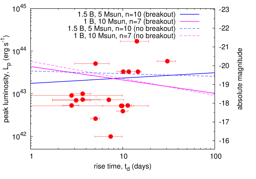
Figure 1.— Rise times and peak luminosities of SNe IIn with analytic relations between the diffusion time $t_{d}$ and the characteristic luminosity $L_{p}$. Data points are based on Table 1 of Ofek et al. (2014a). No bolometric correction is assumed. Characteristic luminosities $L_{p}$ (Eq. 9 for the shock breakout and Eq. 10 for no shock breakout) with two parameter sets are plotted in the figure, ($E_{\mathrm{ej}}$/ 1 B, $M_{\mathrm{ej}}/M_{\odot}$, $n$) $=(1.5,5,10)$ and $(1,10,7)$.

3. Diversity in Type IIn Supernovae

In this section, we investigate the origin of the observational diversities in the rise times and the peak luminosities of SNe IIn and relate these observational diversities to the diversities in the wind density and SN ejecta properties in SNe IIn. We use the analytic estimates for $t_{d}$ and $L_{p}$ obtained in the previous section for this purpose. Ofek et al. (2014a) recently summarized the rise times and peak luminosities of SNe IIn. Based on their Table 1, we plot the rise times and peak luminosities of SNe IIn in Fig. 1. The peak luminosities are based on the $R$ band data and we do not adopt any bolometric corrections in the figure. The bolometric corrections for SNe IIn change with time, but are typically within 0.5 mag and small (Ofek et al., 2014b). We assume that the rise time corresponds to $t_{d}$ and the peak luminosity corresponds to $L_{p}$.

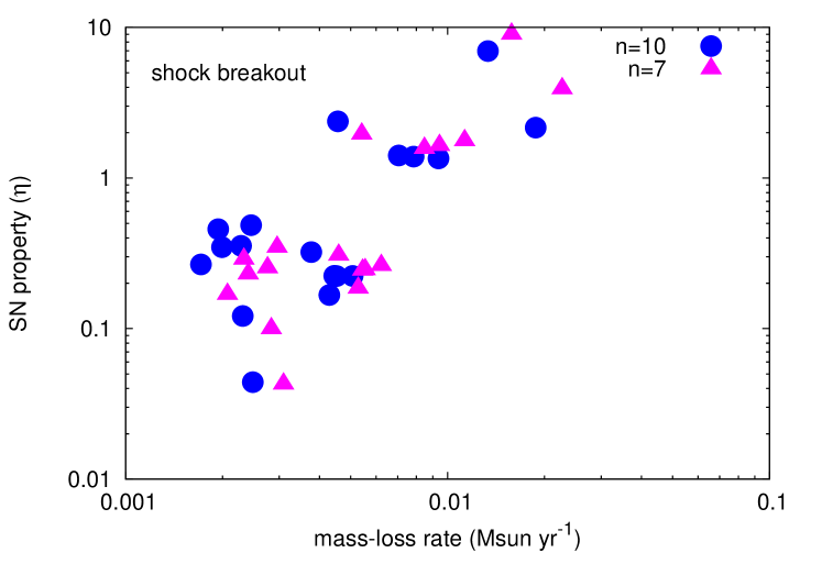
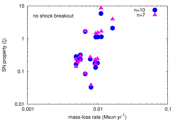
Figure 2.— Diversities in the wind and SN properties in SNe IIn estimated from observed $t_{d}$ and $L_{p}$. The mass-loss rates are estimated with $\dot{M}=4\pi v_{\mathrm{w}}D$ and $v_{\mathrm{w}}=100$ $\mathrm{km~{}s^{-1}}$. The SN properties are $\eta=(M_{\mathrm{ej}}/M_{\mathrm{ej,s}})^{-1.09}(E_{\mathrm{ej}}/E_{\mathrm{ej,s}})^{1.53}$ $(n=10)$ or $\eta=(M_{\mathrm{ej}}/M_{\mathrm{ej,s}})^{-0.657}(E_{\mathrm{ej}}/E_{\mathrm{ej,s}})^{1.31}$ $(n=7)$ (Eq. 11), and $\xi=(M_{\mathrm{ej}}/M_{\mathrm{ej,s}})^{-0.938}(E_{\mathrm{ej}}/E_{\mathrm{ej,s}})^{1.31}$ $(n=10)$ or $\xi=(M_{\mathrm{ej}}/M_{\mathrm{ej,s}})^{-0.6}(E_{\mathrm{ej}}/E_{\mathrm{ej,s}})^{1.2}$ $(n=7)$ (Eq. 13). In our model, $E_{\mathrm{ej},\mathrm{s}}=1.5$ B and $M_{\mathrm{ej},\mathrm{s}}=5$ $M_{\odot}$ for $n=10$ and $E_{\mathrm{ej},\mathrm{s}}=1$ B and $M_{\mathrm{ej},\mathrm{s}}=10$ $M_{\odot}$ for $n=7$. The standard values depend on the model assumptions but the dispersion does not. The left panel shows the parameters for the case of the shock breakout and the right panel shows the region for the case of no shock breakout.

3.1. Diversity in Supernova Ejecta

The analytic estimates for the peak luminosity (Eqs. 9 and 10) show that, if the diffusion time is known, the peak luminosity is mostly determined by the SN properties ($M_{\mathrm{ej}}$ and $E_{\mathrm{ej}}$). In Fig. 1, $L_{p}$ is plotted for two sets of SN ejecta properties, $(E_{\mathrm{ej}}/1\ \mathrm{B},M_{\mathrm{ej}}/M_{\odot},n)=(1.5,5,10)$ and $(1,10,7)$ , for the cases with and without the shock breakout. The conversion efficiency $\epsilon$ is set as 0.3. The suggested conversion efficiency ranges $\epsilon\simeq 0.1-0.5$ in literature and we choose an average value (see, e.g., Fransson et al., 2013). We set $\delta=0$ and choose two $n$ based on the previous studies (e.g., Chevalier & Irwin 2011; Fransson et al. 2013; Matzner & McKee 1999). The characteristic luminosities from the two parameter sets roughly correspond to the average peak luminosity of SNe IIn in Fig. 1. The exact values of $M_{\mathrm{ej}}$ and $E_{\mathrm{ej}}$ which give the average $L_{p}$ depend on the model assumptions like in $\epsilon$ but the diversity does not. As we can see in Fig. 1, $L_{p}$ does not strongly depend on $t_{d}$ and it is in fact mostly determined by the SN ejecta properties. We can see in Fig. 1 that the differences in the observational peak luminosities are roughly within the factors of $0.1-10$ to the analytical average lines. If the shock breakout occurs in the wind, this means that the diversity in the SN properties is roughly within the following range,

$$0.1<\eta\equiv\left(\frac{M_{\mathrm{ej}}}{M_{\mathrm{ej,s}}}\right)^{-\frac{(4n-5)(n-5)}{2n(n-2)}}\left(\frac{E_{\mathrm{ej}}}{E_{\mathrm{ej,s}}}\right)^{\frac{(4n-5)(n-3)}{2n(n-2)}}<10,$$ (15)

where $E_{\mathrm{ej,s}}$ and $M_{\mathrm{ej,s}}$ are the standard values. In our case, $E_{\mathrm{ej,s}}=1.5$ B and $M_{\mathrm{ej,s}}=5\ M_{\odot}$ for $n=10$, and $E_{\mathrm{ej,s}}=1$ B and $M_{\mathrm{ej,s}}=10\ M_{\odot}$ for $n=7$. In Fig. 2, we show the estimated diversity in the SN properties of SNe IIn. For example, if the exploding stars in SNe IIn have similar ejecta mass ($M_{\mathrm{ej}}\simeq M_{\mathrm{ej,s}}$), the ejecta energy needs to be diversified by roughly factors of $0.2-5$ from the standard value. If the ejecta energy is roughly the same in SNe IIn ($E_{\mathrm{ej}}\simeq E_{\mathrm{ej,s}}$), the ejecta mass should be diversified by about factors of $0.1-8$ ($n=10$) or $0.03-40$ ($n=7$) from the standard ejecta mass. Most SNe IIn are found in the observed luminosity range in Fig. 1 (Richardson et al., 2014; Li et al., 2011) and the diversities in SN ejecta properties estimated here are presumed to exist generally in SNe IIn.

So far, we used the shock breakout model to discuss the diversity. The total wind optical depth estimated from Eq. (6) exceeds $\simeq 30$ if $t_{d}\gtrsim 3.5$ days with $R_{i}=10^{13}$ cm $=140\ R_{\odot}$ and the shock breakout may not occur in some SNe IIn shown in Fig. 1, assuming the typical SN shock velocity of 10000 $\mathrm{km~{}s^{-1}}$. The progenitor radius can be larger than 140 $R_{\odot}$ if the progenitor is a RSG or a LBV. Alternatively, if the dense wind is detached and $R_{i}=10^{14}$ cm, for example, the shock breakout only occurs in the SNe IIn with $t_{d}\gtrsim 35$ days. The detachment can occur in SN IIn progenitors if they have variable mass-loss rates. We can see from Fig. 1 that most SNe IIn have $t_{d}$ which is less than 35 days. Assuming $R_{i}=10^{14}$ cm, the observational diversity indicates

$$0.1<\xi\equiv\left(\frac{M_{\mathrm{ej}}}{M_{\mathrm{ej,s}}}\right)^{-\frac{3(n-5)}{2(n-2)}}\left(\frac{E_{\mathrm{ej}}}{E_{\mathrm{ej,s}}}\right)^{\frac{3(n-3)}{2(n-2)}}<10.$$ (16)

The expected diversity does not differ much from that expected from the shock breakout model (Fig. 2). However, $L_{p}$ also depends on $R_{i}$ in this case. The difference in $R_{i}$ by a factor 10 can make the difference in the luminosity by a factor about 2 (Eq. 10).

Whether the shock breakout occurs in the wind also strongly depends on the shock velocity. If the shock velocity is 5000 $\mathrm{km~{}s^{-1}}$, the shock breakout occurs in SNe IIn with $t_{d}>14$ days even in the wind $R_{i}=10^{13}$ cm $=140\ R_{\odot}$, which is compatible with RSG and LBV radii. Then, both SNe IIn with and without the shock breakout may commonly exist (Fig. 1). Ofek et al. (2014a) assumed that the shock breakout always occurs in the dense wind of SNe IIn and they tried to constrain $v_{\mathrm{s}}$ by using the relation $\tau_{\mathrm{w}}\simeq c/v_{\mathrm{s}}$. However, it does not necessarily occur in every SN IIn. Photon diffusion in the wind without the shock breakout may occur commonly in SNe IIn.

Fig. 2 indicates that there may exist two separate populations in the ejecta properties, since SNe IIn do not exist at $\eta\simeq 1$ nor $\xi\simeq 1$. However, the number of the observations is still small and this remains to be investigated.

3.2. Diversity in Wind

If the shock breakout occurs in the dense wind in SNe IIn, the diffusion time $t_{d}$ depends both on the wind properties and the SN ejecta properties (Eq. 5) but it is more sensitive to the wind density. The wind density can be estimated with Eq. (12) by $t_{d}$ and $L_{p}$. Fig. 2 shows the mass-loss rates of SN IIn progenitors obtained by the estimated wind density ($\dot{M}=4\pi v_{\mathrm{w}}D$). We find that the wind density in SNe IIn differs by roughly factors of $0.2-2$ from the average when the shock breakout occurs for the standard sets of $M_{\mathrm{ej}}$ and $E_{\mathrm{ej}}$. The estimated mass-loss rates in Fig. 2 ranges $\sim 10^{-3}-\sim 10^{-2}$ $M_{\odot}~{}\mathrm{yr^{-1}}$ and they are consistent with those estimated in the previous SN IIn studies (e.g., Fox et al. 2011; Kiewe et al. 2012; Taddia et al. 2013; Moriya et al. 2014).

If the shock breakout does not occur in the wind, the wind density can be estimated solely from $t_{d}$ with Eq. (14). Since $t_{d}$ in Fig. 1 are roughly between 1 day and 30 days, the corresponding diversity in the wind density is by factors of $0.3-1.7$, assuming a constant $R_{i}$ and the average $t_{d}$ of 15 days. If $R_{i}=10^{14}$ cm, we obtain $D=1.5\times 10^{15}$ $\mathrm{g~{}cm^{-1}}$ for $t_{d}=1$ day and $D=8.2\times 10^{15}$ $\mathrm{g~{}cm^{-1}}$ for $t_{d}=30$ days. Fig. 1 shows that most $t_{d}$ is between 1 day and 30 days in SNe IIn and the wind density is presumed to differ by factors of $0.3-1.7$ if $R_{i}$ is constant. If the wind velocity $v_{\mathrm{w}}$ is 100 $\mathrm{km~{}s^{-1}}$, the corresponding mass-loss rates of the progenitors are $2.9\times 10^{-3}$ $M_{\odot}~{}\mathrm{yr^{-1}}$ and $1.6\times 10^{-2}$ $M_{\odot}~{}\mathrm{yr^{-1}}$, respectively (Fig. 2).

4. Superluminous Supernovae

The peak magnitudes of superluminous SNe (SLSNe) are brighter than $-21$ mag or roughly $10^{44}$ $\mathrm{erg~{}s^{-1}}$ (Gal-Yam, 2012). Quimby et al. (2013) constructed the pseudo-bolometric LCs of SLSNe. The rise times of SLSNe IIn are typically larger than 40 days. This means that SLSNe IIn have both large $t_{d}$ and $L_{p}$. The large diffusion time indicates that the wind is generally dense enough to cause the shock breakout in SLSNe as is suggested by previous works (e.g., Chevalier & Irwin 2011). The peak luminosities are typically more than about one order of magnitude larger than our standard $L_{p}$ in Fig. 1. We have shown that the peak luminosity does not strongly depend on the wind properties in the shock breakout model and it is mostly determined by the SN ejecta properties. This means that, if the SN ejecta mass of SLSNe is similar to other SNe IIn, their SN kinetic energy needs to be higher by more than a factor of 5 to explain the huge luminosities (Eq. 15). Alternatively, the SN ejecta mass can be smaller by a factor of less than 0.1 $(n=10)$ or 0.03 $(n=7)$ if their SN ejecta energy is similar to the standard SNe IIn. The total emitted energy just by radiation in SLSNe IIn is typically more than $10^{51}$ erg and it is likely that the SN energy is higher than usual SNe.

We show that the large peak luminosities in SLSNe suggest large $E_{\mathrm{ej}}$ and/or small $M_{\mathrm{ej}}$. However, looking at Table 1, we find that larger $E_{\mathrm{ej}}$ and smaller $M_{\mathrm{ej}}$ both make $t_{d}$ smaller. However, $t_{d}$ in SLSNe IIn is much larger than those of SNe IIn. To make large $t_{d}$ with large $E_{\mathrm{ej}}$ and/or small $M_{\mathrm{ej}}$, the wind density must be very large. This indicates that the extremely large explosion energy (and/or the extremely small ejecta mass) as well as the extremely dense wind is required to explain both the large diffusion times and luminosities of SLSNe. Energetic explosions (and/or explosions with very small mass) need to be somehow accompanied by the formation of the dense wind. Detailed modeling of SLSNe also indicates the necessity of high explosion energy in the extremely dense wind (e.g., Ginzburg & Balberg 2012; Moriya et al. 2013a; Chatzopoulos et al. 2013).

5. Conclusions

We have investigated the diversities in rise times and peak luminosities in SNe IIn and related them to the diversities in the wind and SN properties. We have shown that the peak luminosities are mostly affected by the SN properties. The rise times which we relate to the diffusion time $t_{d}$ in the wind can be used to estimate the wind properties individually. We also note that the shock breakout does not necessarily occur in the wind, especially if the progenitors are RSGs or LBVs, and we investigate the models with and without the shock breakout.

The expected diversity in SN ejecta properties estimated from the diversity in the SN IIn peak luminosities is shown in Fig. 2. If the SN ejecta mass does not differ much in SNe IIn, the diversity in the SN ejecta energy is by factors of $0.2-5$ from the average. If the SN ejecta energy is similar in SNe IIn, the diversity in the SN ejecta mass is expected to be by factors of $0.1-8$ $(n=10)$ or $0.03-40$ $(n=7)$ from the average. The expected diversity does not strongly differ if we assume that the shock breakout occurs in the wind or not.

The diversity in the wind density can be estimated with the diversity in the rise times (Fig. 2). If the shock breakout occurs in the wind, the expected diversity in the wind density for SNe IIn with similar peak luminosities is by factors of $0.2-2$ from the average. If the shock breakout does not occur, the diversity is factors of $0.3-1.7$ from the average.

SLSNe IIn show both the large peak luminosities and the large rise times. We suggest that both the high wind density and the high explosion energy and/or small ejecta mass are required to explain the properties of the SLSNe. The large rise times indicate that the shock breakout occurs in the wind in the SLSNe. The large peak luminosities indicate that the explosion energy is very large and/or the ejecta mass is very small. However, the large explosion energy and/or small ejecta mass make the diffusion time smaller. Thus, the large wind density is required to have the large rise times. Putting together, not only the larger wind density but also the larger SN energy and/or the smaller SN ejecta mass than typical SNe IIn are required to have the large peak luminosities and large rise times at the same time as observed in SLSNe.

Appendix A Constants

Constants which appear in the main text are

$$C_{1}=\left[\frac{1}{2\pi(n-4)(n-3)(n-\delta)}\frac{\left[2(5-\delta)(n-5)\right]^{\frac{n-3}{2}}}{\left[(3-\delta)(n-3)\right]^{\frac{n-5}{2}}}\right]^{\frac{1}{n-2}},$$ (A1)

$$C_{2}=c^{-\frac{1}{n-2}}\left[2\pi(n-4)(n-3)(n-\delta)\frac{[(3-\delta)(n-3)]^{\frac{n-5}{2}}}{[2(5-\delta)(n-5)]^{\frac{n-3}{2}}}\right]^{\frac{1}{n-2}}\left(\frac{n-2}{n-3}\right)^{\frac{n-3}{n-2}},$$ (A2)

$$C_{3}=\frac{2\pi}{n-5}c^{\frac{n-5}{n(n-2)}}\left[\frac{1}{4\pi(n-\delta)}\frac{\left[2(5-\delta)(n-5)\right]^{\frac{n-3}{2}}}{\left[(3-\delta)(n-3)\right]^{\frac{n-5}{2}}}\right]^{\frac{4n-5}{n(n-2)}}\left[\frac{(n-4)(n-3)}{2}\right]^{\frac{(n-1)(n-5)}{n(n-2)}}\left(\frac{n-3}{n-2}\right)^{\frac{(n-5)(n-3)}{n(n-2)}},$$ (A3)

and

$$C_{4}=\frac{2\pi}{n-5}c^{\frac{n-5}{2(n-2)}}\left[\frac{1}{4\pi(n-\delta)}\frac{\left[2(5-\delta)(n-5)\right]^{\frac{n-3}{2}}}{\left[(3-\delta)(n-3)\right]^{\frac{n-5}{2}}}\right]^{\frac{3}{n-2}}\left[\frac{(n-4)(n-3)}{2}\right]^{\frac{n-5}{n-2}}.$$ (A4)

References

- Chatzopoulos et al. (2013) Chatzopoulos, E., Wheeler, J. C., Vinko, J., Horvath, Z. L., & Nagy, A. 2013, ApJ, 773, 76
- Chevalier (1982) Chevalier, R. A. 1982, ApJ, 258, 790
- Chevalier & Irwin (2011) Chevalier, R. A., & Irwin, C. M. 2011, ApJ, 729, L6
- Filippenko (1997) Filippenko, A. V. 1997, ARA&A, 35, 309
- Fox et al. (2011) Fox, O. D., Chevalier, R. A., Skrutskie, M. F., et al. 2011, ApJ, 741, 7
- Fransson et al. (2013) Fransson, C., Ergon, M., Challis, P. J., et al. 2013, arXiv:1312.6617
- Gal-Yam (2012) Gal-Yam, A. 2012, Science, 337, 927
- Ginzburg & Balberg (2012) Ginzburg, S., & Balberg, S. 2012, ApJ, 757, 178
- Kiewe et al. (2012) Kiewe, M., Gal-Yam, A., Arcavi, I., et al. 2012, ApJ, 744, 10
- Langer (2012) Langer, N. 2012, ARA&A, 50, 107
- Li et al. (2011) Li, W., Leaman, J., Chornock, R., et al. 2011, MNRAS, 412, 1441
- Matzner & McKee (1999) Matzner, C. D., & McKee, C. F. 1999, ApJ, 510, 379
- Moriya et al. (2014) Moriya, T. J., Maeda, K., Taddia, F., et al. 2014, MNRAS, 439, 2917
- Moriya et al. (2013a) Moriya, T. J., Blinnikov, S. I., Tominaga, N., et al. 2013a, MNRAS, 428, 1020
- Moriya et al. (2013b) Moriya, T. J., Maeda, K., Taddia, F., et al. 2013b, MNRAS, 435, 1520
- Ofek et al. (2014a) Ofek, E. O., Arcavi, I., Tal, D., et al. 2014a, ApJ, 788, 154
- Ofek et al. (2014b) Ofek, E. O., Zoglauer, A., Boggs, S. E., et al. 2014b, ApJ, 781, 42
- Quimby et al. (2013) Quimby, R. M., Yuan, F., Akerlof, C., & Wheeler, J. C. 2013, MNRAS, 431, 912
- Richardson et al. (2014) Richardson, D., Jenkins, R. L., III, Wright, J., & Maddox, L. 2014, AJ, 147, 118
- Schlegel (1990) Schlegel, E. M. 1990, MNRAS, 244, 269
- Taddia et al. (2013) Taddia, F., Stritzinger, M. D., Sollerman, J., et al. 2013, A&A, 555, A10