$B\to\rho$ semileptonic decays and $|V_{ub}|$

Abstract

We reevaluate the $B\to\rho\,l^{+}\nu_{l}$ decay width as a full $B\to\pi\pi\,l^{+}\nu_{l}$ four-particle decay, in which the two final pions are produced via an intermediate $\rho$ meson. The decay width can be written as a convolution of the $B\to\rho\,l^{+}\nu_{l}$ decay width, for an off-shell $\rho$, with the $\rho\to\pi\pi$ line shape. This allows to fully incorporate the effects of the finite $\rho$ meson width. As shown, consideration of the $\rho$ meson width effects increase the $|V_{ub}|$ value by some 8%, rendering it in better agreement with the determination based in the $B\to\pi$ decay. We take the $q^{2}$ dependence of the $B\to\rho$ semileptonic form factors from a dispersive Omnès representation. The Omnès subtraction constants and the overall normalization parameter $|V_{ub}|$ are fitted to light cone sum rules and lattice QCD theoretical form-factor calculations, in the low and high $q^{2}$ regions respectively, together to the CLEO, BaBar and Belle experimental partial branching fraction distributions. The extracted value from this global fit is $|V_{ub}|=(3.12\pm 0.13)\times 10^{-3}$, in agreement with the average $B\to\pi$ exclusive value $|V_{ub}|=(3.23\pm 0.31)\times 10^{-3}$ quoted by the Particle Data Group. The extracted value increases to $|V_{ub}|=(3.51\pm 0.16)\times 10^{-3}$ if only the most recent Belle Collaboration data is used. This latter value is in agreement with different theoretical determinations based in the $B\to\pi$ semileptonic decay and the values obtained by the CKMfitter and UTfit groups. In any case a clear tension with the $|V_{ub}|$ value extracted from inclusive semileptonic $b\to u$ decays still persists.

I Introduction

A precise determination of $V_{ub}$ is essential to check the consistency of the Standard Model, especially the description of $CP$ violations. However, $V_{ub}$ is still the least well known element of the Cabibbo-Kobayashi-Maskawa (CKM) matrix. At present, there is a clear tension between the $|V_{ub}|$ values extracted from the analysis of inclusive and exclusive decays. Determinations based on inclusive semileptonic decays have their largest uncertainties coming from the error on the $b-$ quark mass, but their values tend to be consistent. From these analyses, the average value quoted by the Particle Data Group (PDG) in its 2013 update Beringer:1900zz is $|V_{ub}|=(4.41\pm 0.15^{+0.15}_{-0.17})\times 10^{-3}$. The corresponding average value extracted from exclusive determinations is dominated by the $B\to\pi$ semileptonic decay value $|V_{ub}|=(3.23\pm 0.31)\times 10^{-3}$ Beringer:1900zz . In this case the error is dominated by form factor normalizations. Another problem which will be addressed here, is the existing tension between the exclusive determinations using the $B\to\rho$ and $B\to\pi$ semileptonic decays. From $B\to\rho$ decays lower values have been traditionally reported, thus for instance, BaBar presented a value of $|V_{ub}|=(2.75\pm 0.24)\times 10^{-3}$ in delAmoSanchez:2010af , while in the approach of Ref. Flynn:2008zr , similar to the one followed here and based on the Omnès representation of the form factors, was obtained $|V_{ub}|=(2.76\pm 0.21)\times 10^{-3}$. Very recent analyses, using light cone sum rules (LCSR), also find central values, $|V_{ub}|=(2.91\pm 0.19)\times 10^{-3}$ and $|V_{ub}|=(3.11\pm 0.19)\times 10^{-3}$  Fu:2014pba , below those found from $B\to\pi$ decays ($|V_{ub}|=(3.47\pm 0.29\pm 0.03)\times 10^{-3}$ Flynn:2007ii , $|V_{ub}|=(3.6\pm 0.4_{\rm stat}\pm 0.2^{+0.6}_{{\rm syst}-0.4{\rm thy}})\times 10^{-3}$ Adam:2007pv , $|V_{ub}|=(3.41^{+0.37}_{-0.32}|_{\rm th}\pm 0.06|_{\rm exp})\times 10^{-3}$  Khodjamirian:2011ub , $|V_{ub}|=(3.52\pm 0.29)\times 10^{-3}$ Sibidanov:2013rkk ). As pointed out in Ref. Meissner:2013pba , part of this systematic discrepancy could be due to the fact that the $B\to\rho$ analyses do not take into account the effect of the broad $\rho-$width.

In Ref. Kang:2013jaa the authors propose to extract $|V_{ub}|$ from the analysis of the four-body semileptonic decay $B\to\pi\pi l^{+}\nu_{l}$ taking into account $\pi\pi$ rescattering effects and the effect of the rho meson. Their approach is based on dispersion theory and does not rely on specific resonant contributions. In our calculation we do a simpler study of the four-body decay in which the two pions are produced via an intermediate $\rho$ meson $B\to\pi\pi(\rho)l^{+}\nu_{l}$. The decay width can then be expressed as an integration over the $\rho$ meson invariant mass available in the $B\to\rho\,l^{+}\nu_{l}$ decay for an off-shell $\rho$, weighted by the $\rho\to\pi\pi$ line shape distribution that fully takes into account $\rho$ meson width effects. In fact, this type of analysis has been recently done by the Belle collaboration in Ref. Sibidanov:2013rkk with the result that a larger $|V_{ub}|$ value, in better agreement with the determination from $B\to\pi$ semileptonic decay, is obtained.

In this work we perform a combined fit to the latest partial branching fraction distributions by the different experimental collaborations, while at the same time we substantially improve on the treatment of the form factors over previous works. In this respect we shall follow Ref. Flynn:2008zr , where the $B\to\rho$ form factors are described using a multiply subtracted Omnès dispersion relation. The Omnès functional form depends on the form factor values at the subtraction points and those values are treated as free parameters. These, together with $|V_{ub}|$, are fitted both to $B\to\rho\,l^{+}\nu_{l}$ recent partial branching fraction measurements from Belle Sibidanov:2013rkk , BaBar delAmoSanchez:2010af and CLEO Gray:2007pw collaborations, as well as to theoretical results for the $B\to\rho$ form factors obtained using LCSR Ball:2004rg and lattice calculations by the SPQcdR Abada:2002ie and UKQCD Bowler:2004zb collaborations. For the $\rho\to\pi\pi$ decay we use a phenomenological vertex where the coupling constant has been fixed to the on-shell $\rho$ meson decay width.

The paper is organized as follows. In Sec.II we present all the expressions needed to evaluate the decay width. We shall give a triple differential decay width distribution with respect to $p_{\rho}^{2},q^{2}$ and $x_{l}$, with $p_{\rho}^{2}$ the $\rho$ meson invariant mass square, $q$ the total four-momentum of the final lepton system, and $x_{l}$ the cosinus of the angle formed by the momentum of the charged lepton, measured in the lepton center of mass system, and the momentum of the virtual $\rho$ in the $B$ meson rest frame. These are the variables used by the experiments, and in order to obtain the fractional branching fractions (see below) we just have to integrate over their corresponding ranges. Sec. III describes the fitting procedure that follows closely Ref. Flynn:2008zr , and finally, in Sec. IV we present and discuss the main results of this work. In Appendix A, we give details on the helicity amplitude formalism used to evaluate the product of the leptonic and hadronic tensors, while in Appendix B we provide the correlation matrix resulting from our global fit.

II $\Gamma[B\to\pi\pi(\rho)\,l^{+}\nu_{l}]$ decay width

Working in the exact isospin limit, the $B\to\pi\pi(\rho)\,l^{+}\nu_{l}$ decay width is given by

$$\Gamma=\left(\frac{G_{F}}{\sqrt{2}}\right)^{2}|V_{ub}|^{2}C_{\rho}^{2}\frac{1}{2m_{B}}\frac{1}{(2\pi)^{8}}\int\frac{d^{3}p_{l}}{2E_{l}}\int\frac{d^{3}p_{\nu}}{2E_{\nu}}\int\frac{d^{3}p_{\pi_{1}}}{2E_{\pi_{1}}}\int\frac{d^{3}p_{\pi_{2}}}{2E_{\pi_{2}}}\,\delta^{(4)}(p_{B}-p_{l}-p_{\nu}-p_{\pi_{1}}-p_{\pi_{2}})$$

$$\hskip 56.9055pt\times\sum_{s_{l}}\sum_{s_{\nu}}\Big{|}h_{\alpha\sigma}(p_{B},p_{\rho})\frac{-g^{\sigma\beta}+\frac{p_{\rho}^{\sigma}p_{\rho}^{\beta}}{p_{\rho}^{2}}}{p_{\rho}^{2}-m_{\rho}^{2}+i\sqrt{p_{\rho}^{2}}\,\Gamma_{\rho}(p_{\rho}^{2})}(p_{\pi_{1}}-p_{\pi_{2}})_{\beta}\,\bar{u}_{s_{\nu}}(p_{\nu})\gamma^{\alpha}(1-\gamma_{5})v_{s_{l}}(p_{l})\Big{|}^{2},$$ (1)

where only the transverse part of the $\rho$ meson propagator contributes in that limit LopezCastro:1999xg . $G_{F}=1.166378\times 10^{-5}\,$GeV^-2 Beringer:1900zz is the Fermi decay constant and $C_{\rho}=6$ is the effective $\rho\to\pi\pi$ coupling constant with

$$\Gamma_{\rho}(p_{\rho}^{2})=\frac{C_{\rho}^{2}}{6\pi\,p_{\rho}^{2}}\Big{(}\frac{p_{\rho}^{2}}{4}-m_{\pi}^{2}\Big{)}^{3/2}$$ (2)

being the $\rho$ meson width for $\sqrt{p_{\rho}^{2}}$ invariant mass. Besides, $p_{B}=(m_{B},\vec{0}\,)$, $p_{\rho}=p_{B}-p_{l}-p_{\nu}$ and

$$h_{\alpha\sigma}(p_{B},p_{\rho}) = \frac{2V(q^{2})}{m_{B}+\sqrt{p_{\rho}^{2}}}\,\epsilon_{\alpha\gamma\delta\sigma}p_{B}^{\gamma}p_{\rho}^{\delta}-i(m_{B}+\sqrt{p_{\rho}^{2}}\,)A_{1}(q^{2})\,g_{\alpha\sigma}$$ (3)

$$+i\frac{A_{2}(q^{2})}{m_{b}+\sqrt{p_{\rho}^{2}}}\,q_{\sigma}(p_{B}+p_{\rho})_{\alpha}\,-i\frac{2A(q^{2})}{q^{2}}\sqrt{p_{\rho}^{2}}\ q_{\alpha}(p_{B}+p_{\rho})_{\sigma},$$

where $V$ and $A_{1},A_{2},A$ are respectively the vector and axial form factors for the $B\to\rho$ weak transition. Here we use $\epsilon_{0123}=+1$ and we have defined $q=p_{B}-p_{\rho}=p_{l}+p_{\nu}$, which is the total four-momentum carried by the leptons. In the above expression for $h_{\alpha\sigma}$ we have substituted $m_{\rho}$ by $\sqrt{p_{\rho}^{2}}$ with respect to the corresponding expression in Ref. Flynn:2008zr
The above expression for $\Gamma$ can be rewritten as

$$\Gamma = \left(\frac{G_{F}}{\sqrt{2}}\right)^{2}|V_{ub}|^{2}\frac{1}{m_{B}}\frac{1}{(2\pi)^{6}}\int\frac{d^{3}p_{l}}{E_{l}}\int\frac{d^{3}p_{\nu}}{E_{\nu}}\ {\cal L}^{\alpha\alpha^{\prime}}(p_{l},p_{\nu})$$ (4)

$$\hskip 56.9055pt\times\sum_{r=\pm 1,0}\sum_{s=\pm 1,0}\frac{h_{\alpha\sigma}(p_{B},p_{\rho})\epsilon_{r}^{\sigma\,*}(p_{\rho})h^{*}_{\alpha^{\prime}\sigma^{\prime}}(p_{B},p_{\rho})\epsilon_{s}^{\sigma^{\prime}\,}(p_{\rho})}{|p_{\rho}^{2}-m_{\rho}^{2}+i\sqrt{p_{\rho}^{2}}\,\Gamma_{\rho}(p_{\rho}^{2})|^{2}}\ 2\sqrt{p_{\rho}^{2}}\,\Gamma_{\rho}^{rs}(p_{\rho}^{2})$$

where we have used that

$$\big{(}-g^{\sigma\beta}+\frac{p_{\rho}^{\sigma}p_{\rho}^{\beta}}{p_{\rho}^{2}}\Big{)}=\sum_{r=\pm 1,0}\epsilon_{r}^{\sigma\,*}(p_{\rho})\epsilon_{r}^{\beta}(p_{\rho}),$$ (5)

with $\epsilon_{r}(p_{\rho}),\,r=\pm 1,0$ the three polarization vectors of a $\rho$ meson with invariant mass given by $\sqrt{p_{\rho}^{2}}$. ${\cal L}^{\alpha\alpha^{\prime}}(p_{l},p_{\nu})$ is the lepton tensor given by

$${\cal L}^{\alpha\alpha^{\prime}}(p_{l},p_{\nu})=p_{l}^{\alpha}p_{\nu}^{\alpha^{\prime}}-g^{\alpha\alpha^{\prime}}p_{l}\cdot p_{\nu}+p_{l}^{\alpha^{\prime}}p_{\nu}^{\alpha}\pm i\epsilon^{\gamma\alpha\delta\alpha^{\prime}}p_{l\gamma}p_{\nu\,\delta},$$ (6)

where the $\pm$ sign corresponds to $l^{+}\nu_{l}$ or $l\,\bar{\nu}_{l}$ decays respectively and

$$\Gamma_{\rho}^{rs}(p_{\rho}^{2})=C_{\rho}^{2}\frac{\epsilon_{r}^{\beta}(p_{\rho})\epsilon_{s}^{\beta^{\prime}\,*}(p_{\rho})}{2\sqrt{p_{\rho}^{2}}\,(2\pi)^{2}}\int\frac{d^{3}p_{\pi_{1}}}{2E_{\pi_{1}}}\int\frac{d^{3}p_{\pi_{2}}}{2E_{\pi_{2}}}\delta^{(4)}(p_{\rho}-p_{\pi_{1}}-p_{\pi_{2}})(p_{\pi_{1}}-p_{\pi_{2}})_{\beta}\,(p_{\pi_{1}}-p_{\pi_{2}})_{\beta^{\prime}}.$$ (7)

The integrals in $\Gamma_{\rho}^{rs}(p_{\rho}^{2})$ can be readily evaluated using Lorentz covariance and one gets that

$$\Gamma_{\rho}^{rs}(p_{\rho}^{2})=-\delta_{rs}\,\Gamma_{\rho}(p_{\rho}^{2}),$$ (8)

Then,

$$\Gamma=\left(\frac{G_{F}}{\sqrt{2}}\right)^{2}|V_{ub}|^{2}\frac{1}{m_{B}}\frac{1}{(2\pi)^{5}}\int\frac{d^{3}p_{l}}{E_{l}}\int\frac{d^{3}p_{\nu}}{E_{\nu}}{\cal L}^{\alpha\alpha^{\prime}}(p_{l},p_{\nu})\ {\cal H}_{\alpha\alpha^{\prime}}(p_{B},p_{\rho})\,\delta_{\rho}(p_{\rho}^{2}),$$ (9)

where we have defined the hadronic tensor

$${\cal H}_{\alpha\alpha^{\prime}}(p_{B},p_{\rho})=\sum_{r=\pm 1,0}h_{\alpha\sigma}(p_{B},p_{\rho})\epsilon_{r}^{\sigma\,*}(p_{\rho})h^{*}_{\alpha^{\prime}\sigma^{\prime}}(p_{B},p_{\rho})\epsilon_{r}^{\sigma^{\prime}\,}(p_{\rho}),$$ (10)

and the $\rho$ meson line shape function

$$\delta_{\rho}(p_{\rho}^{2})=\frac{1}{\pi}\frac{\sqrt{p_{\rho}^{2}}\,\Gamma_{\rho}(p_{\rho}^{2})}{|p_{\rho}^{2}-m_{\rho}^{2}+i\sqrt{p_{\rho}^{2}}\,\Gamma_{\rho}(p_{\rho}^{2})|^{2}}.$$ (11)

A representation of the latter as a function of the $\rho$ invariant mass is given in Fig. 1.

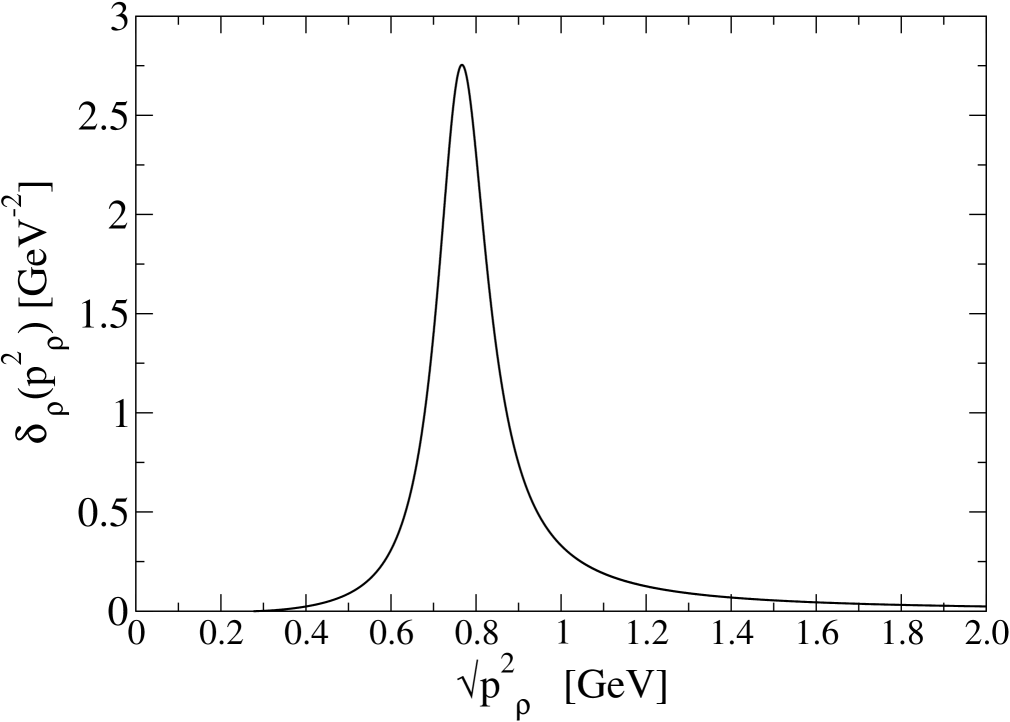
Figure 1: $\delta_{\rho}(p_{\rho}^{2})$ representation as a function of $\sqrt{p_{\rho}^{2}}$.

In the $\Gamma_{\rho}(p_{\rho}^{2})\to 0$ limit, one would have

$$\delta_{\rho}(p_{\rho}^{2})\approx\delta(p_{\rho}^{2}-m_{\rho}^{2}),$$ (12)

and in that case $\Gamma$ would be given by

$$\Gamma \approx \left(\frac{G_{F}}{\sqrt{2}}\right)^{2}|V_{ub}|^{2}\frac{1}{m_{B}}\frac{1}{(2\pi)^{5}}\int\frac{d^{3}p_{l}}{E_{l}}\int\frac{d^{3}p_{\nu}}{E_{\nu}}{\cal L}^{\alpha\alpha^{\prime}}(p_{l},p_{\nu}){\cal H}_{\alpha\alpha^{\prime}}(p_{B},p_{\rho})\,\delta({p_{\rho}^{2}}-m^{2}_{\rho})$$ (13)

$$= \left(\frac{G_{F}}{\sqrt{2}}\right)^{2}|V_{ub}|^{2}\frac{1}{m_{B}}\frac{1}{(2\pi)^{5}}\int\frac{d^{3}p_{l}}{E_{l}}\int\frac{d^{3}p_{\nu}}{E_{\nu}}\int{d^{4}p_{\rho}}\,\delta(p_{\rho}^{2}-m_{\rho}^{2})\delta^{(4)}(p_{B}-p_{l}-p_{\nu}-p_{\rho})\,{\cal L}^{\alpha\alpha^{\prime}}(p_{l},p_{\nu}){\cal H}_{\alpha\alpha^{\prime}}(p_{B},p_{\rho})$$

$$= \left(\frac{G_{F}}{\sqrt{2}}\right)^{2}|V_{ub}|^{2}\frac{1}{m_{B}}\frac{1}{(2\pi)^{5}}\int\frac{d^{3}p_{l}}{E_{l}}\int\frac{d^{3}p_{\nu}}{E_{\nu}}\int\frac{d^{3}p_{\rho}}{2E_{\rho}}\delta^{(4)}(p_{B}-p_{l}-p_{\nu}-p_{\rho})\,{\cal L}^{\alpha\alpha^{\prime}}(p_{l},p_{\nu}){\cal H}_{\alpha\alpha^{\prime}}(p_{B},p_{\rho})$$

$$= \Gamma(B\to\rho\,l^{+}\nu_{l})$$

recovering the expression for the $B\to\rho\,l^{+}\nu_{l}$ decay width used in previous analyses where the $\rho$ meson widths effects were not taken into account.

Going back to the full expression, it can be rewritten as

$$\Gamma = \left(\frac{G_{F}}{\sqrt{2}}\right)^{2}\frac{|V_{ub}|^{2}}{m_{B}(2\pi)^{5}}\int\frac{d^{3}p_{\nu}}{E_{\nu}}\int\frac{d^{3}p_{l}}{E_{l}}{\cal L}^{\alpha\alpha^{\prime}}(p_{l},p_{\nu})\,{\cal H}_{\alpha\alpha^{\prime}}(p_{B},p_{B}-p_{l}-p_{\nu})\,\delta_{\rho}(p_{\rho}^{2})$$

$$= \left(\frac{G_{F}}{\sqrt{2}}\right)^{2}\frac{|V_{ub}|^{2}}{m_{B}(2\pi)^{5}}\int dp_{\rho}^{2}\,\delta_{\rho}(p_{\rho}^{2})\,\int\frac{d^{3}p_{\rho}}{2E_{\rho}}\,\int\frac{d^{3}p_{\nu}}{E_{\nu}}\int\frac{d^{3}p_{l}}{E_{l}}{\cal L}^{\alpha\alpha^{\prime}}(p_{l},p_{\nu})\,{\cal H}_{\alpha\alpha^{\prime}}(p_{B},p_{\rho})\delta^{(4)}(p_{B}-p_{\rho}-p_{l}-p_{\nu})$$

with $E_{\rho}=p_{\rho}^{0}=\sqrt{p_{\rho}^{2}+\vec{p}_{\rho}^{\ {}^{2}}}$. Then,

$$\Gamma = \int dp_{\rho}^{2}\,\delta_{\rho}(p_{\rho}^{2})\,\Big{\{}\left(\frac{G_{F}}{\sqrt{2}}\right)^{2}\frac{|V_{ub}|^{2}}{m_{B}(2\pi)^{5}}\int\frac{d^{3}p_{\rho}}{2E_{\rho}}\int\frac{d^{3}p_{\nu}}{E_{\nu}}\int\frac{d^{3}p_{l}}{E_{l}}{\cal L}^{\alpha\alpha^{\prime}}(p_{l},p_{\nu})\,{\cal H}_{\alpha\alpha^{\prime}}(p_{B},p_{\rho})\delta^{(4)}(p_{B}-p_{\rho}-p_{l}-p_{\nu})\Big{\}},$$

where the term in curly brackets represents the $B\to\rho\,l^{+}\nu_{l}$ decay width for the case of a final $\rho$ meson with invariant mass $\sqrt{p_{\rho}^{2}}$. The integrals on neutrino variables can be evaluated using Lorentz covariance

$$\int\frac{d^{3}p_{\nu}}{E_{\nu}}\int\frac{d^{3}p_{l}}{E_{l}}{\cal L}^{\alpha\alpha^{\prime}}(p_{l},p_{\nu})\,{\cal H}_{\alpha\alpha^{\prime}}(p_{B},p_{\rho})\delta^{(4)}(q-p_{l}-p_{\nu})=2\pi\frac{q^{2}-m_{l}^{2}}{2q^{2}}\int_{-1}^{1}dx_{l}\,{\cal L}^{\alpha\alpha^{\prime}}(\tilde{p}_{l},\tilde{p}_{\nu}){\cal H}_{\alpha\alpha^{\prime}}(\Lambda p_{B},\Lambda p_{\rho}),$$ (15)

where $\Lambda$ is a rotation that takes $\vec{p}_{\rho}$ to the negative $Z$ axis followed by a boost to the center of mass of the two final leptons. In that case

$$\Lambda p_{B} = \frac{1}{2\sqrt{q^{2}}}\,\Big{(}m_{B}^{2}+q^{2}-p_{\rho}^{2},0,0,-\lambda^{1/2}(m_{B}^{2},q^{2},p_{\rho}^{2})\Big{)},$$

$$\Lambda p_{\rho} = \frac{1}{2\sqrt{q^{2}}}\,\Big{(}{m_{B}^{2}-q^{2}-p_{\rho}^{2}},0,0,-\lambda^{1/2}(m_{B}^{2},q^{2},p_{\rho}^{2})\Big{)}.$$ (16)

It is clear now that the product of tensors ${\cal L}^{\alpha\alpha^{\prime}}(\tilde{p}_{l},\tilde{p}_{\nu}){\cal H}_{\alpha\alpha^{\prime}}(\Lambda p_{B},\Lambda p_{\rho})$ does not depend on the lepton $\varphi_{l}$ azimuthal angle that can then be integrated out to give a factor $2\pi$. The lepton $\tilde{p}_{l}$ and $\tilde{p}_{\nu}$ momenta can be chosen for simplicity as

$$\tilde{p}_{l}=(\frac{q^{2}+m_{l}^{2}}{2\sqrt{q^{2}}},\frac{q^{2}-m_{l}^{2}}{2\sqrt{q^{2}}}\sqrt{1-x_{l}^{2}},0,-\frac{q^{2}-m_{l}^{2}}{2\sqrt{q^{2}}}x_{l}),$$ (17)

$$\tilde{p}_{\nu}=(\frac{q^{2}-m_{l}^{2}}{2\sqrt{q^{2}}},-\frac{q^{2}-m_{l}^{2}}{2\sqrt{q^{2}}}\sqrt{1-x_{l}^{2}},0,\frac{q^{2}-m_{l}^{2}}{2\sqrt{q^{2}}}x_{l}).$$ (18)

With this definition, $x_{l}$ is the cosinus of the angle formed by the momentum of the charged lepton measured in the center of mass of the two leptons, with the direction of the momentum of the virtual $\rho$ meson measured in the reference frame in which the $B$ meson is at rest. Since there is no dependence on the $\vec{p}_{\rho}$ angular variables we find

$$\Gamma = \int dp_{\rho}^{2}\,\delta_{\rho}(p_{\rho}^{2})\,\Big{\{}\left(\frac{G_{F}}{\sqrt{2}}\right)^{2}\frac{|V_{ub}|^{2}}{2m_{B}(2\pi)^{3}}\int\frac{\lambda^{1/2}(m_{B}^{2},q^{2},p_{\rho}^{2})}{2m_{B}}dE_{\rho}\frac{q^{2}-m_{l}^{2}}{2q^{2}}\int_{-1}^{1}dx_{l}\,{\cal L}^{\alpha\alpha^{\prime}}(\tilde{p}_{l},\tilde{p}_{\nu}){\cal H}_{\alpha\alpha^{\prime}}(\Lambda p_{B},\Lambda p_{\rho})\Big{\}},$$ (19)

from where one can write the following differential decay width

$$\frac{d\Gamma}{dp_{\rho}^{2}\,dq^{2}\,dx_{l}}=\delta_{\rho}(p_{\rho}^{2})\,\frac{G_{F}^{2}|V_{ub}|^{2}}{128\pi^{3}m_{B}^{3}q^{2}}\lambda^{1/2}(m_{B}^{2},q^{2},p_{\rho}^{2})({q^{2}-m_{l}^{2}})\,{\cal L}^{\alpha\alpha^{\prime}}(\tilde{p}_{l},\tilde{p}_{\nu})\,{\cal H}_{\alpha\alpha^{\prime}}(\Lambda p_{B},\Lambda p_{\rho}).$$ (20)

The product ${\cal L}^{\alpha\alpha^{\prime}}(\tilde{p}_{l},\tilde{p}_{\nu})\,{\cal H}_{\alpha\alpha^{\prime}}(\Lambda p_{B},\Lambda p_{\rho})$ can be evaluated using the formalism of helicity amplitudes (see for instance Ref. Ivanov:2005fd ) that we discuss in Appendix A. The final expression for the triple differential decay width is

$$\frac{d\Gamma}{dp_{\rho}^{2}\,dq^{2}\,dx_{l}} = \delta_{\rho}(p_{\rho}^{2})\,\frac{G_{F}^{2}|V_{ub}|^{2}}{512\pi^{3}m_{B}^{3}q^{2}}\lambda^{1/2}(m_{B}^{2},q^{2},p_{\rho}^{2})({q^{2}-m_{l}^{2}})^{2}$$ (21)

$$\hskip 28.45274pt\times\Big{\{}\ 2(1-x_{l}^{2})H_{00}+(1\mp x_{l})^{2}H_{+1+1}+(1\pm x_{l})^{2}H_{-1-1}$$

$$\hskip 42.67912pt+\frac{m_{l}^{2}}{q^{2}}[(1-x_{l}^{2})(H_{+1+1}+H_{-1-1})+2x_{l}^{2}H_{00}+2H_{tt}+4x_{l}H_{t0}]\Big{\}}.$$

where the different $H_{rs}$ hadronic helicity amplitudes are defined and given in Appendix A. Besides de upper sign corresponds to $l^{+}\nu_{l}$ decays, like experiments in Refs. Gray:2007pw ; delAmoSanchez:2010af ; Hokuue:2006nr , while the lower sign corresponds to $l^{-}\bar{\nu}_{l}$ ones, like in the latest Belle Sibidanov:2013rkk analysis. This difference is only relevant if the integration over $x_{l}$ does not cover its full range $[-1,1]$ as in the case of CLEO data Gray:2007pw . Neglecting lepton masses, a good approximation for light $l=e,\mu$ final leptons, one arrives at the expression

$$\frac{d\Gamma}{dp_{\rho}^{2}\,dq^{2}\,dx_{l}}\approx\delta_{\rho}(p_{\rho}^{2})\,\frac{G_{F}^{2}|V_{ub}|^{2}}{512\pi^{3}m_{B}^{3}}q^{2}\lambda^{1/2}(q^{2},m_{B}^{2},p_{\rho}^{2})\Big{[}2(1-x_{l})^{2}\,{\cal H}_{00}+(1\mp x_{l})^{2}\,{\cal H}_{+1+1}+(1\pm x_{l})^{2}\,{\cal H}_{-1-1}\Big{]}.$$ (22)

where the corresponding helicity amplitudes depend only on the $V(q^{2}),A_{1}(q^{2})$ and $A_{2}(q^{2})$ form factors.

III Fitting procedure

The fitting procedure that we shall use is, with minor modifications, the one followed in Ref. Flynn:2008zr . We describe our $B\to\rho$ form factors using a multiply subtracted Omnès dispersion relation omnes1 ; omnes2 , the latter being based in unitarity and analyticity. We will have

$$F(q^{2})=\frac{1}{s_{0}-q^{2}}\prod_{j=0}^{n}[F(q_{j}^{2})(s_{0}-q_{j}^{2})]^{\alpha_{j}(q^{2})}\ \ ,\ \ \alpha_{j}(q^{2})=\prod_{\stackrel{{\scriptstyle k=0}}{{k\neq j}}}^{n}\frac{q^{2}-q_{k}^{2}}{q_{j}^{2}-q_{k}^{2}},\ \ F=V,A_{1},A_{2}.$$ (23)

$s_{0}$ corresponds to the pole of the form factor and we shall use $s_{0}=m_{B^{*}}=5.3252\,$GeV Beringer:1900zz for the vector form factor and $s_{0}=5.7235$ GeV Beringer:1900zz (the mass of the $1^{+}$ B meson) for the two axial form factors. As in Ref. Flynn:2008zr , we use three subtraction points at $q^{2}=0,\,2q^{2}_{\rm max}/3,\,q^{2}_{\rm max}$ where we take $q^{2}_{max}=(m_{B}-m_{\rho})^{2}=20.3\,$GeV² as used in Refs. Gray:2007pw ; delAmoSanchez:2010af ; Hokuue:2006nr . Note however the latest Belle analysis in Ref. Sibidanov:2013rkk works with $q^{2}$ values up to 22-24 GeV². The values of $F(0),F(2q^{2}_{\rm max}/3)$ and $F(q^{2}_{\rm max})$, for $F=V,A_{1},A_{2}$, are treated as free parameters as will be $|V_{ub}|$. The values of these ten parameters are then fitted to reproduce form factor theoretical results obtained in LCSR Ball:2004rg and lattice calculations Abada:2002ie ; Bowler:2004zb , and experimental measurements of partial branching fractions obtained by the CLEO Gray:2007pw , BaBar delAmoSanchez:2010af and Belle Sibidanov:2013rkk collaborations. The partial branching fractions are defined as

$$B=\frac{1}{\Gamma(B^{0})}\int_{p_{\rho\,{\rm inf}}^{2}}^{p_{\rho\,{\rm sup}}^{2}}dp_{\rho}^{2}\int_{q^{2}_{\rm inf}}^{q^{2}_{\rm sup}}dq^{2}\int_{x_{l\,{\rm inf}}}^{x_{l\,{\rm sup}}}dx_{l}\,\frac{d\Gamma}{dp_{\rho}^{2}\,dq^{2}\,dx_{l}},$$ (24)

where for the $B^{0}$ lifetime we use $\tau_{0}=1/\Gamma(B^{0})=(1.519\pm 0.007)\times 10^{-12}\,$s Beringer:1900zz . It is worth mentioning that even though the different experiments select $\rho$ events in a reduced $\sqrt{p_{\rho}^{2}}$ interval, this is treated as an overall acceptance effect that it is corrected in the final data bernlochner . Thus, one has that $p_{\rho\,{\rm sup}}^{2}=(m_{B}-m_{l})^{2}$ and $p_{\rho\,{\rm inf}}^{2}=4m_{\pi}^{2}$. For the lower (inf) and upper (sup) limits in $q^{2}$ and $x_{l}$ we use the values provided by the experiments (see Table 1). For the $B^{+}$ lifetime to be used below we take $\tau_{+}=(1.641\pm 0.008)\times 10^{-12}\,$s Beringer:1900zz .

III.1 Experimental and theoretical input

Experimental data by the CLEO Gray:2007pw , BaBar delAmoSanchez:2010af and Belle Sibidanov:2013rkk collaborations consist of partial branching fractions as defined in Eq.(24). Their values together with statistical and systematic errors are collected in Table 1. CLEO has made used of isospin symmetry to combine results for neutral and charged $B$ meson decays. For BaBar data we have combined their $B^{0}\to\rho^{-}l^{+}\nu_{l}$ 4-mode and $B^{+}\to\rho^{0}l^{+}\nu_{l}$ data in the following way: Denoting as $\sigma$ and $\epsilon$ the statistical and systematic errors respectively we have evaluated

$$\frac{1}{\sigma^{2}} = \frac{1}{\sigma^{2}_{\rho^{-}}}+\frac{1}{(2\frac{\tau_{0}}{\tau_{+}}\,\sigma_{\rho^{0}})^{2}},$$

$$\frac{1}{\epsilon^{2}} = \frac{1}{\epsilon^{2}_{\rho^{-}}}+\frac{1}{(2\frac{\tau_{0}}{\tau_{+}}\,\epsilon_{\rho^{0}})^{2}},$$

$$\frac{B}{\sigma^{2}+\epsilon^{2}} = \frac{B_{\rho^{-}}}{\sigma^{2}_{\rho^{-}}+\epsilon^{2}_{\rho^{-}}}+\frac{2\frac{\tau_{0}}{\tau_{+}}\,B_{\rho^{0}}}{(2\frac{\tau_{0}}{\tau_{+}}\,\sigma_{\rho^{0}})^{2}+(2\frac{\tau_{0}}{\tau_{+}}\,\epsilon_{\rho^{0}})^{2}}$$ (25)

In the case o the newest Belle’s data Sibidanov:2013rkk we treat separately the neutral and charge meson decays since they have been evaluated for different $q^{2}$ bins. However in order to perform the fit we multiply the $\rho^{0}$ data by $2\tau_{0}/\tau_{+}$.

	$q^{2}\,[{\rm GeV^{2}}]$	$x_{l}$	$10^{4}B$
CLEO Gray:2007pw	$0-2$	$[-1,1]$	$0.45\pm 0.20\pm 0.15$
	$2-8$	$[-1,1]$	$0.96\pm 0.20\pm 0.29$
	$8-16$	$[0,1]$	$0.75\pm 0.16\pm 0.14$
	$16-20.3$	$[0,1]$	$0.35\pm 0.07\pm 0.05$
	$8-20.3$	$[-1,0]$	$0.42\pm 0.18\pm 0.31$
BaBar delAmoSanchez:2010af	$0-8$	$[-1,1]$	$0.587\pm 0.084\pm 0.097$
	$8-16$	$[-1,1]$	$0.928\pm 0.047\pm 0.103$
	$16-20.3$	$[-1,1]$	$0.263\pm 0.017\pm 0.042$
Belle Sibidanov:2013rkk
$\rho^{+}$ data	$0-4$	$[-1,1]$	$0.373\pm 0.106$
	$4-8$	$[-1,1]$	$0.718\pm 0.116$
	$8-12$	$[-1,1]$	$0.806\pm 0.123$
	$12-16$	$[-1,1]$	$0.723\pm 0.125$
	$16-20$	$[-1,1]$	$0.626\pm 0.115$
	$20-24$	$[-1,1]$	$0.017\pm 0.079$
$\rho^{0}$ data $\times\ 2\tau_{0}/\tau_{+}$	$0-2$	$[-1,1]$	$0.2296\pm 0.0629$
	$2-4$	$[-1,1]$	$0.2851\pm 0.0574$
	$4-6$	$[-1,1]$	$0.3314\pm 0.0629$
	$6-8$	$[-1,1]$	$0.4017\pm 0.0629$
	$8-10$	$[-1,1]$	$0.2647\pm 0.0537$
	$10-12$	$[-1,1]$	$0.3684\pm 0.0629$
	$12-14$	$[-1,1]$	$0.4147\pm 0.0629$
	$14-16$	$[-1,1]$	$0.4017\pm 0.0611$
	$16-18$	$[-1,1]$	$0.3240\pm 0.0592$
	$18-20$	$[-1,1]$	$0.2647\pm 0.0180$
	$20-22$	$[-1,1]$	$0.1092\pm 0.0481$

Table 1: Experimental partial branching fractions used as input. The different $q^{2}$ and $x_{l}$ intervals are shown. Belle’s original $\rho^{0}$ data in Ref. Sibidanov:2013rkk is shown multiplied by the factor $2\tau_{0}/\tau_{+}$.

The theoretical input consists of form factors values. For $q^{2}$ in the $[0,10]\,$GeV² range we will use the LCSR form factor values obtained from the parameterizations given in Ref. Ball:2004rg . For higher $q^{2}$ we will use the lattice results by the SPQcdR  Abada:2002ie and UKQCD Bowler:2004zb collaborations. All of them are collected in Table 2. For the LCSR form factors, and following Ref. delAmoSanchez:2010af , we have assumed a 10% error at $q^{2}=0$ that increases linearly to 13% at $q^{2}=14\,{\rm GeV}^{2}$. SPQcdR errors include both systematic and statistical uncertainties while in the case of UKQCD data both statistical and systematic errors are shown. The latter are highly asymmetric. Following Ref. Flynn:2008zr , and in order to perform the fit, we put the UKQCD form factors values in the center of their systematic range and we use half that range as the systematic error.

	$q^{2}\,[{\rm GeV}^{2}]$	$V$	$A_{1}$	$A_{2}$
LCSR Ball:2004rg	0	$0.324\pm 0.032$	$0.240\pm 0.024$	$0.221\pm 0.022$
	1	$0.343\pm 0.035$	$0.247\pm 0.025$	$0.232\pm 0.024$
	2	$0.364\pm 0.038$	$0.254\pm 0.026$	$0.244\pm 0.025$
	3	$0.387\pm 0.041$	$0.261\pm 0.028$	$0.257\pm 0.027$
	4	$0.412\pm 0.045$	$0.269\pm 0.029$	$0.271\pm 0.029$
	5	$0.440\pm 0.049$	$0.277\pm 0.031$	$0.286\pm 0.032$
	6	$0.471\pm 0.053$	$0.286\pm 0.032$	$0.302\pm 0.034$
	7	$0.506\pm 0.058$	$0.295\pm 0.034$	$0.320\pm 0.037$
	8	$0.546\pm 0.064$	$0.305\pm 0.036$	$0.339\pm 0.040$
	9	$0.590\pm 0.070$	$0.316\pm 0.038$	$0.360\pm 0.043$
	10	$0.641\pm 0.078$	$0.327\pm 0.040$	$0.384\pm 0.047$
SPQcdR Abada:2002ie	10.69	$0.51\pm 0.26$	$0.354\pm 0.085$	$0.38\pm 0.26$
	12.02	$0.61\pm 0.28$	$0.384\pm 0.087$	$0.49\pm 0.30$
	13.35	$0.74\pm 0.30$	$0.421\pm 0.089$	$0.65\pm 0.35$
	14.68	$0.93\pm 0.31$	$0.465\pm 0.092$	$0.93\pm 0.41$
	16.01	$1.20\pm 0.32$	$0.519\pm 0.097$	$1.41\pm 0.56$
	17.34	$1.61\pm 0.33$	$0.588\pm 0.108$	$2.39\pm 1.23$
	18.67	$2.26\pm 0.55$	$0.678\pm 0.134$	$4.7\pm 4.1$
UKQCD Bowler:2004zb	$12.67$	$0.684\pm 0.162^{+0.00}_{-0.56}$	$0.439\pm 0.067^{+0.000}_{-0.080}$	$0.70\pm 0.49^{+0.08}_{-0.03}$
	$13.01$	$0.714\pm 0.162^{+0.00}_{-0.50}$	$0.448\pm 0.065^{+0.000}_{-0.079}$	$0.71\pm 0.46^{+0.08}_{-0.03}$
	$13.51$	$0.763\pm 0.155^{+0.00}_{-0.40}$	$0.460\pm 0.063^{+0.000}_{-0.075}$	$0.72\pm 0.43^{+0.10}_{-0.02}$
	$14.02$	$0.818\pm 0.147^{+0.00}_{-0.31}$	$0.472\pm 0.059^{+0.000}_{-0.073}$	$0.73\pm 0.42^{+0.12}_{-0.01}$
	$14.52$	$0.883\pm 0.141^{+0.00}_{-0.24}$	$0.485\pm 0.055^{+0.000}_{-0.070}$	$0.76\pm 0.42^{+0.14}_{-0.03}$
	$15.03$	$0.967\pm 0.137^{+0.00}_{-0.20}$	$0.498\pm 0.051^{+0.000}_{-0.068}$	$0.78\pm 0.46^{+0.16}_{-0.05}$
	$15.53$	$1.057\pm 0.134^{+0.00}_{-0.19}$	$0.513\pm 0.049^{+0.000}_{-0.067}$	$0.81\pm 0.54^{+0.18}_{-0.06}$
	$16.04$	$1.164\pm 0.150^{+0.10}_{-0.21}$	$0.529\pm 0.047^{+0.000}_{-0.066}$	$0.84\pm 0.71^{+0.20}_{-0.07}$
	$16.54$	$1.296\pm 0.184^{+0.21}_{-0.25}$	$0.544\pm 0.043^{+0.000}_{-0.062}$	$0.87\pm 0.97^{+0.23}_{-0.08}$
	$17.05$	$1.46\pm 0.26^{+0.34}_{-0.30}$	$0.560\pm 0.043^{+0.000}_{-0.059}$	$0.90\pm 1.35^{+0.27}_{-0.07}$
	$17.55$	$1.67\pm 0.40^{+0.49}_{-0.36}$	$0.577\pm 0.043^{+0.000}_{-0.058}$	$0.90\pm 1.89^{+0.33}_{-0.03}$
	$16.54$	$2.02\pm 0.68^{+0.73}_{-0.48}$	$0.599\pm 0.052^{+0.000}_{-0.058}$	$0.9\pm 2.9^{+0.4}_{-0.1}$

Table 2: Theoretical form factor inputs used for the fit. SPQcdR and UKQCD data taken from Table 2 in Ref. Flynn:2008zr . Concerning UKQCD data see text for details.

III.2 $\chi^{2}$ definition

The $\chi^{2}$ function we use for the fit is

$$\chi^{2}=\sum_{j,k=1}^{115}[(Q^{\rm input}_{j}-Q^{\rm fit}_{j})C^{-1}_{jk}(Q^{\rm input}_{k}-Q^{\rm fit}_{k})]$$ (26)

where $Q^{\rm input}_{j}$ represents any of the input quantities and $Q^{\rm fit}_{j}$ is the corresponding value obtained in our calculation. In order to construct the $C$ covariant matrix we have not considered any correlation between data from different experiments or between different theoretical calculations, or between experimental and theoretical inputs. $C$ is then block diagonal. CLEO and BaBar collaborations provide statistical and systematic correlation matrices and in these two cases their corresponding blocks in $C$ are constructed as

$$C_{jk}=\sigma_{j}\sigma_{k}{\cal C}^{\rm stat}_{jk}+\epsilon_{j}\epsilon_{k}{\cal C}^{\rm sys}_{jk}.$$ (27)

with ${\cal C}^{{\rm stat}/{\rm sys}}$ the statistical/systematic correlation matrices. The Belle Collaboration Sibidanov:2013rkk also provides two independent statistical correlation matrices, one for $\rho^{+}$ data and one for $\rho^{0}$ data, so that we build two independent blocks as

$$C_{jk}=\sigma_{j}\sigma_{k}{\cal C}^{\rm stat}_{jk}.$$ (28)

For the block corresponding to UKQCD data we use

$$C_{jk}=\sigma^{2}_{j}\delta_{jk}+\epsilon_{j}\epsilon_{k},$$ (29)

that assumes independent statistical uncertainties and fully correlated systematic errors. Finally for LCSR and SPQcdR results we use

$$C_{jk}=\sigma^{2}_{j}\delta_{jk}.$$ (30)

IV Results and discussion

Best fit results are compiled in Table 3.

$|V_{ub}|$	$(3.12\pm 0.13)\times 10^{-3}$
$V(0)$	$0.349\pm 0.022$
$V(2q^{2}_{\rm max}/3)$	$0.863\pm 0.042$
$V(q^{2}_{\rm max})$	$2.553\pm 0.375$
$A_{1}(0)$	$0.253\pm 0.011$
$A_{1}(2q^{2}_{\rm max}/3)$	$0.429\pm 0.013$
$A_{1}(q^{2}_{\rm max})$	$0.719\pm 0.038$
$A_{2}(0)$	$0.226\pm 0.014$
$A_{2}(2q^{2}_{\rm max}/3)$	$0.701\pm 0.065$
$A_{2}(q^{2}_{\rm max})$	$3.033\pm 0.914$

Table 3: Best fit parameters of the global fit.

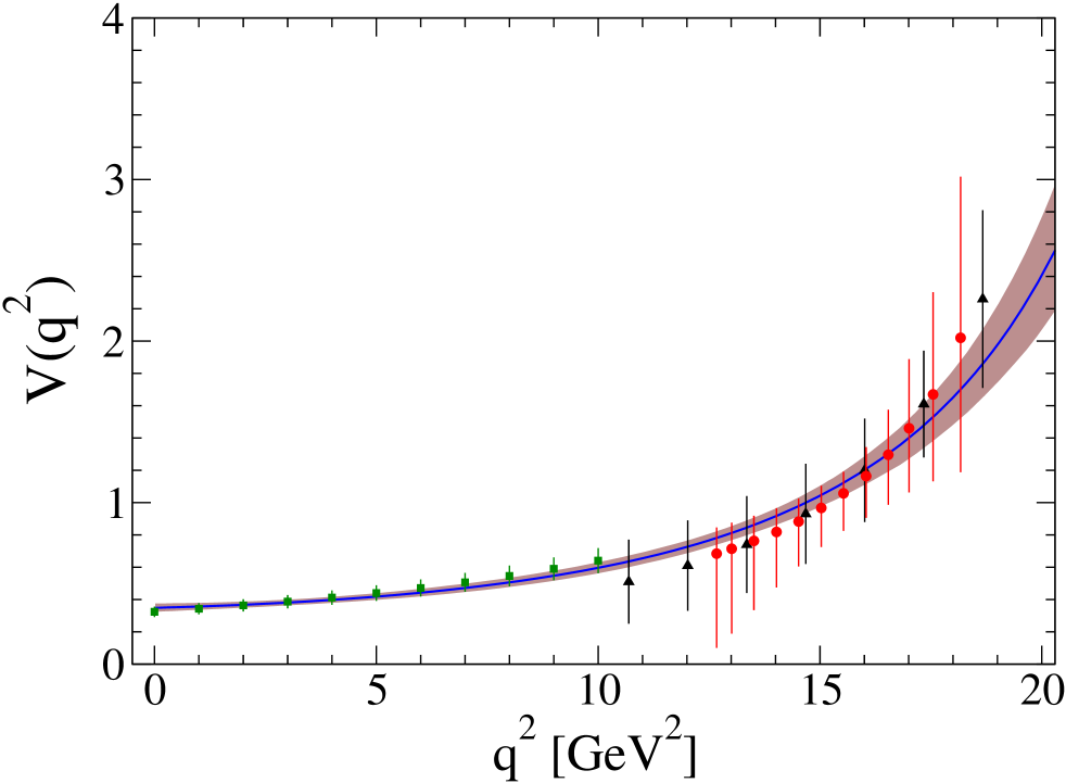
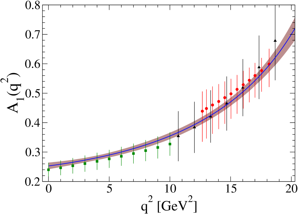
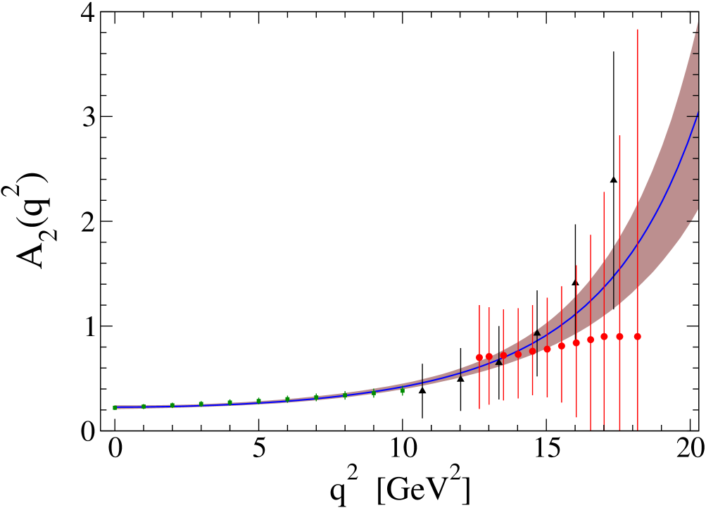
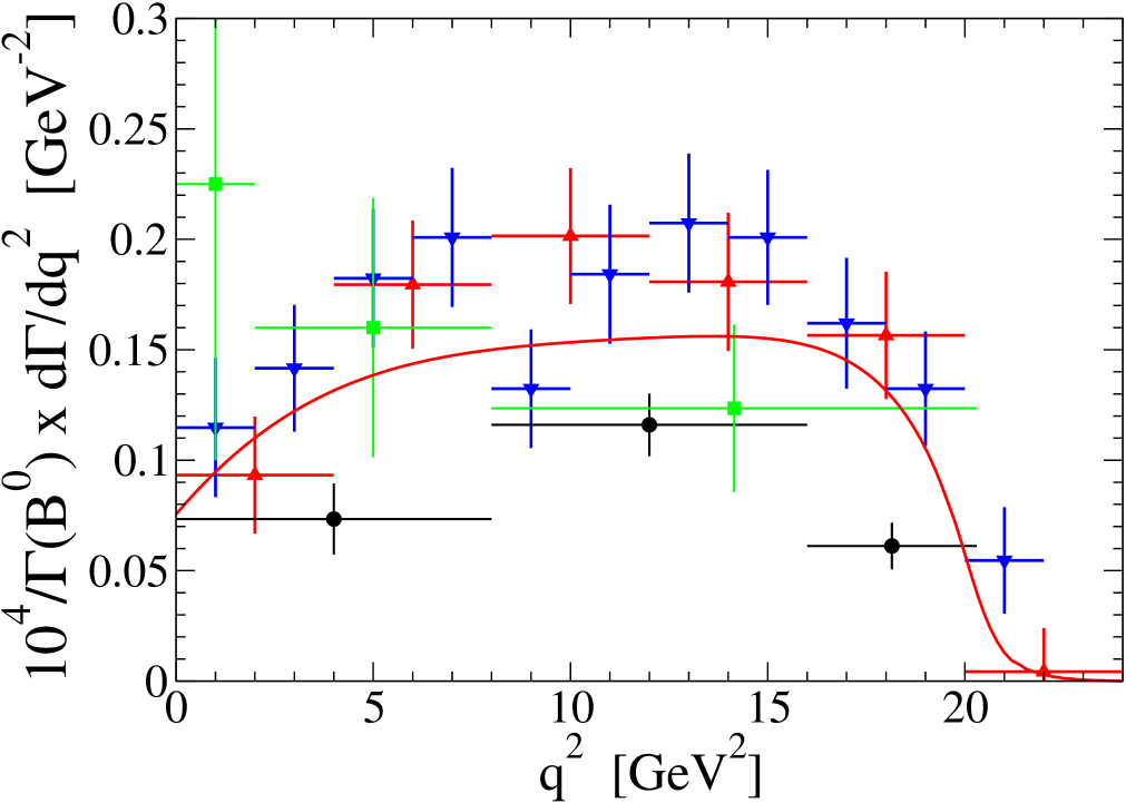
Figure 2: Top panels and left-bottom panel: Form factor obtained from the fit (solid line) together with their corresponding 68% confidence level band. We show the predictions from LCSR Ball:2004rg (squares), and lattice QCD from the SPQcdR Abada:2002ie (up-triangles) and UKQCD Bowler:2004zb (circles) collaborations. Right-bottom panel: $\frac{10^{4}}{\Gamma(B^{0})}\frac{d\Gamma}{dq^{2}}[{\rm GeV}^{-2}]$. Up-triangles, down-triangles, circles, and squares stand respectively for Belle $\rho^{+}$ and $\rho^{0}$ data Sibidanov:2013rkk , BaBar data delAmoSanchez:2010af , and CLEO data Gray:2007pw . The solid line stands for our prediction.

The fit has $\chi^{2}/{\rm d.o.f.}=1.6$ for a total of 105 degrees of freedom. The corresponding Gaussian correlation matrix is given in Appendix B. The value $|V_{ub}|=(3.12\pm 0.13)\times 10^{-3}$ extracted from our global fit analysis is in agreement with the average determination from the exclusive $B\to\pi$ decays given by $(3.23\pm 0.31)\times 10^{-3}$ Beringer:1900zz . A calculation based in Eq.(13), i.e. ignoring $\rho$ meson width effects, would have provided a smaller value of $|V_{ub}|=(2.87\pm 0.13)\times 10^{-3}$.

In Fig. 2 we show the form factors, together with their 68% confidence level bands, that result from the global fit, and we compare them to the different theoretical input. Finally in Fig. 2 (bottom-right panel) we also present our prediction for $\frac{10^{4}}{\Gamma(B^{0})}\frac{d\Gamma}{dq^{2}}$ and compare it to data by the Belle Sibidanov:2013rkk , BaBar delAmoSanchez:2010af , and CLEO Gray:2007pw collaborations. The largest discrepancy occurs for CLEO data where the experimental distribution peaks a significantly smaller $q^{2}$ values than the theoretical distribution. This seems to be incompatible with the theoretical form factor predictions at low $q^{2}$ obtained in LCSR. Belle and BaBar results agree better in shape with our analysis. However, one clearly sees in Fig. 2 that BaBar data would prefer a smaller $|V_{ub}|$ value, whereas Belle data would be better reproduced with a higher $|V_{ub}|$ value.

The recent data by the Belle Collaboration Sibidanov:2013rkk gives results for smaller $q^{2}$ bins which means more data and then the possibility for more stringent constraints on theoretical models. In this respect it is worth making a fit just to Belle’s data together with the form factors. In this case one gets $|V_{ub}|=(3.51\pm 0.16)\times 10^{-3}$ which is in perfect agreement with the analyses in Ref. Sibidanov:2013rkk where other sets of form factors were used. A fit to the form factors and to the BaBar data of Ref. delAmoSanchez:2010af alone would give $|V_{ub}|=(2.52\pm 0.18)\times 10^{-3}$ which is much smaller than the result obtained from Belle data. Note also that the total decay rate from BaBar extracted in Ref. delAmoSanchez:2010af is some 15% smaller that the one provided in their earlier measurement of Ref. Aubert:2005cd and used in Flynn:2008zr .

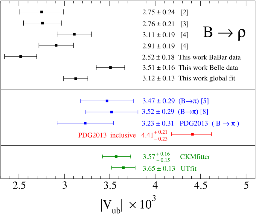
Figure 3: Different $|V_{ub}|$ values obtained in $B\to\rho$ decay analyses. We also show for comparison the $|V_{ub}|$ determination from the $B\to\pi$ decay in Refs. Flynn:2007ii ; Sibidanov:2013rkk , the PDG exclusive and inclusive 2013 average updates Beringer:1900zz , and the fits from the CKMfitter ckmfitter and UTfit utfit groups.

In Fig. 3 we show different $|V_{ub}|$ values obtained in $B\to\rho$ decay analyses. As mentioned, our global fit result is in agreement with the $B\to\pi$ exclusive decay average value quoted in the PDG 2013 update Beringer:1900zz . The results by the CKMfitter ckmfitter and UTfit utfit groups are in very good agreement with our determination using only the recent Belle data. However, as seen in Fig. 3, there still persist the large discrepancy between inclusive and exclusive determinations of $|V_{ub}|$, with the global fits by the CKMfitter ckmfitter and UTfit utfit groups being in better agreement with the latter.

Appendix A Helicity amplitudes

In this appendix we shall write the product ${\cal L}^{\alpha\alpha^{\prime}}(\tilde{p}_{l},\tilde{p}_{\nu}){\cal H}_{\alpha\alpha^{\prime}}(\Lambda p_{B},\Lambda p_{\rho})$ in terms of helicity amplitudes. For that purpose we use that

$$g^{\mu\nu}=\sum_{r=t,\pm 1,0}g_{rr}\,\epsilon_{r}^{\mu}(\Lambda q)\epsilon_{r}^{\nu\,*}(\Lambda q)=\sum_{r=t,\pm 1,0}g_{rr}\,\epsilon_{r}^{\mu\,*}(\Lambda q)\epsilon_{r}^{\nu}(\Lambda q),$$ (31)

with $g_{tt}=-g_{+1+1}=-g_{-1-1}=-g_{00}=1$ and

$$\epsilon_{t}(\Lambda q) = \frac{\Lambda q}{\sqrt{q^{2}}}=(1,0,0,0),$$ (32)

$$\epsilon_{+1}(\Lambda q) = \Big{(}0,\frac{-1}{\sqrt{2}},\frac{-i}{\sqrt{2}},0\Big{)},$$ (33)

$$\epsilon_{-1}(\Lambda q) = \Big{(}0,\frac{1}{\sqrt{2}},\frac{-i}{\sqrt{2}},0\Big{)},$$ (34)

$$\epsilon_{0}(\Lambda q) = (0,0,0,1).$$ (35)

Then,

$${\cal L}^{\alpha\alpha^{\prime}}(\tilde{p}_{l},\tilde{p}_{\nu})\,{\cal H}_{\alpha\alpha^{\prime}}(\Lambda p_{B},\Lambda p_{\rho})=\sum_{r=t,\pm 1,0}\sum_{s=t,\pm 1,0}g_{rr}g_{ss}\,{\cal L}_{rs}(\tilde{p}_{l},\tilde{p}_{\nu})\,{\cal H}_{rs}(\Lambda p_{B},\Lambda p_{\rho}),$$ (36)

where we have defined the hadronic and leptonic helicity amplitudes

$${\cal H}_{rs}(\Lambda p_{B},\Lambda p_{\rho}) = \epsilon_{r}^{\alpha\,*}(\Lambda q)\,{\cal H}_{\alpha\alpha^{\prime}}(\Lambda p_{B},\Lambda p_{\rho})\,\epsilon_{s}^{\alpha^{\prime}}(\Lambda q),$$ (37)

$${\cal L}_{rs}(\tilde{p}_{l},\tilde{p}_{\nu}) = \epsilon_{r}^{\beta}(\Lambda q)\,{\cal L}_{\beta\beta^{\prime}}(\tilde{p}_{l},\tilde{p}_{\nu})\,\epsilon_{s}^{\beta^{\prime}\,*}(\Lambda q).$$ (38)

As

$${\cal H}_{\alpha\alpha^{\prime}}(\Lambda p_{B},\Lambda p_{\rho})=\sum_{u=\pm 1,0}h_{\alpha\sigma}(\Lambda p_{B},\Lambda p_{\rho})\epsilon_{u}^{\sigma\,*}(\Lambda p_{\rho})h_{\alpha^{\prime}\sigma^{\prime}}^{*}(\Lambda p_{B},\Lambda p_{\rho})\epsilon_{u}^{\sigma^{\prime}}(\Lambda p_{\rho}),$$ (39)

we will have

$${\cal H}_{rs}(\Lambda p_{B},\Lambda p_{\rho}) = \sum_{u=\pm 1,0}\epsilon_{r}^{\alpha\,*}(\Lambda q)h_{\alpha\sigma}(\Lambda p_{B},\Lambda p_{\rho})\epsilon_{u}^{\sigma\,*}(\Lambda p_{\rho})\epsilon_{s}^{\alpha^{\prime}}(\Lambda q)h_{\alpha^{\prime}\sigma^{\prime}}^{*}(\Lambda p_{B},\Lambda p_{\rho})\epsilon_{u}^{\sigma^{\prime}}(\Lambda p_{\rho})$$ (40)

$$= \sum_{u=\pm 1,0}h_{ru}(\Lambda p_{B},\Lambda p_{\rho})h_{su}^{*}(\Lambda p_{B},\Lambda p_{\rho}),$$ (41)

with

$$h_{ru}(\Lambda p_{B},\Lambda p_{\rho})=\epsilon_{r}^{\alpha\,*}(\Lambda q)h_{\alpha\sigma}(\Lambda p_{B},\Lambda p_{\rho})\epsilon_{u}^{\sigma\,*}(\Lambda p_{\rho}).$$ (42)

Using

$$\epsilon_{+1}(\Lambda p_{\rho}) = \Big{(}0,\frac{-1}{\sqrt{2}},\frac{-i}{\sqrt{2}},0\Big{)},$$ (43)

$$\epsilon_{-1}(\Lambda p_{\rho}) = \Big{(}0,\frac{1}{\sqrt{2}},\frac{-i}{\sqrt{2}},0\Big{)},$$ (44)

$$\epsilon_{0}(\Lambda p_{\rho}) = \Big{(}\frac{\lambda^{1/2}(q^{2},m_{B}^{2},p_{\rho}^{2})}{2\sqrt{q^{2}}\sqrt{p_{\rho}^{2}}},0,0,-\frac{m_{B}^{2}-q^{2}-p_{\rho}^{2}}{2\sqrt{q^{2}}\sqrt{p_{\rho}^{2}}}\Big{)}.$$ (45)

we can evaluate the $h_{ru}$ quantities. The nonzero ones are

$$h_{t0} = \frac{\lambda^{1/2}(m_{B}^{2},q^{2},p_{\rho}^{2})}{2\sqrt{p_{\rho}^{2}}\sqrt{q^{2}}}\Big{[}-iA_{1}(q^{2})\Big{(}m_{B}+\sqrt{p_{\rho}^{2}}\,\Big{)}+iA_{2}(q^{2})\Big{(}m_{B}-\sqrt{p_{\rho}^{2}}\ \Big{)}-i2A(q^{2})\sqrt{p_{\rho}^{2}}\ \Big{]},$$

$$h_{+1-1} = -iA_{1}(q^{2})\Big{(}m_{B}+\sqrt{p_{\rho}^{2}}\,\Big{)}+iV(q^{2})\frac{\lambda^{1/2}(m_{B}^{2},q^{2},p_{\rho}^{2})}{m_{B}+\sqrt{p_{\rho}^{2}}},$$

$$h_{-1+1} = -iA_{1}(q^{2})\Big{(}m_{B}+\sqrt{p_{\rho}^{2}}\,\Big{)}-iV(q^{2})\frac{\lambda^{1/2}(m_{B}^{2},q^{2},p_{\rho}^{2})}{m_{B}+\sqrt{p_{\rho}^{2}}},$$

$$h_{00} = \frac{1}{2\sqrt{p_{\rho}^{2}}\sqrt{q^{2}}}\Big{[}-iA_{1}(q^{2})\Big{(}m_{B}+\sqrt{p_{\rho}^{2}}\,\Big{)}(m_{B}^{2}-p_{\rho}^{2}-q^{2})+i\frac{A_{2}(q^{2})\lambda(m_{B}^{2},q^{2},p_{\rho}^{2})}{m_{B}+\sqrt{p_{\rho}^{2}}}\,\Big{]}.$$ (46)

From these values we get the following nonzero hadronic helicity amplitudes

$${\cal H}_{tt} = \frac{\lambda(m_{B}^{2},q^{2},p_{\rho}^{2})}{4\,{p_{\rho}^{2}}\,{q^{2}}}\left[-A_{1}(q^{2})\Big{(}m_{B}+\sqrt{p_{\rho}^{2}}\,\Big{)}+A_{2}(q^{2})\Big{(}m_{B}-\sqrt{p_{\rho}^{2}}\,\Big{)}-2A(q^{2})\sqrt{p_{\rho}^{2}}\ \right]^{2},$$

$${\cal H}_{t0}={\cal H}_{0t} = \frac{\lambda^{1/2}(m_{B}^{2},q^{2},p_{\rho}^{2})}{4\,{p_{\rho}^{2}}\,{q^{2}}}\Big{[}-A_{1}(q^{2})\Big{(}m_{B}+\sqrt{p_{\rho}^{2}}\,\Big{)}(m_{B}^{2}-p_{\rho}^{2}-q^{2})+\frac{A_{2}(q^{2})\lambda(m_{B}^{2},q^{2},p_{\rho}^{2})}{m_{B}+\sqrt{p_{\rho}^{2}}}\ \Big{]}$$

$$\hskip 14.22636pt\times\Big{[}-A_{1}(q^{2})\Big{(}m_{B}+\sqrt{p_{\rho}^{2}}\,\Big{)}+A_{2}(q^{2})\Big{(}m_{B}-\sqrt{p_{\rho}^{2}}\,\Big{)}-2A(q^{2})\sqrt{p_{\rho}^{2}}\ \Big{]},$$

$${\cal H}_{00} = \frac{1}{4\,{p_{\rho}^{2}}\,{q^{2}}}\Big{[}-A_{1}(q^{2})\Big{(}m_{B}+\sqrt{p_{\rho}^{2}}\,\Big{)}(m_{B}^{2}-p_{\rho}^{2}-q^{2})+\frac{A_{2}(q^{2})\lambda(m_{B}^{2},q^{2},p_{\rho}^{2})}{m_{B}+\sqrt{p_{\rho}^{2}}}\ \Big{]}^{2},$$

$${\cal H}_{+1+1} = \Big{[}A_{1}(q^{2})\Big{(}m_{B}+\sqrt{p_{\rho}^{2}}\,\Big{)}-V(q^{2})\frac{\lambda^{1/2}(m_{B}^{2},q^{2},p_{\rho}^{2})}{m_{B}+\sqrt{p_{\rho}^{2}}}\ \Big{]}^{2},$$

$${\cal H}_{-1-1} = \Big{[}A_{1}(q^{2})\Big{(}m_{B}+\sqrt{p_{\rho}^{2}}\,\Big{)}+V(q^{2})\frac{\lambda^{1/2}(m_{B}^{2},q^{2},p_{\rho}^{2})}{m_{B}+\sqrt{p_{\rho}^{2}}}\ \Big{]}^{2}.$$ (47)

The corresponding leptonic helicity amplitudes are given by

$${\cal L}_{tt} = (q^{2}-m_{l}^{2})\frac{m_{l}^{2}}{2\,{q^{2}}},$$

$${\cal L}_{t0}={\cal L}_{0t} = -(q^{2}-m_{l}^{2})x_{l}\frac{m_{l}^{2}}{2\,{q^{2}}},$$

$${\cal L}_{00} = (q^{2}-m_{l}^{2})\frac{1}{2}\Big{[}1-x_{l}^{2}+x_{l}^{2}\frac{m_{l}^{2}}{q^{2}}\Big{]},$$

$${\cal L}_{+1+1} = (q^{2}-m_{l}^{2})\frac{1}{4}\Big{[}(1\mp x_{l})^{2}+(1-x_{l}^{2})\,\frac{m_{l}^{2}}{q^{2}}\Big{]},$$

$${\cal L}_{-1-1} = (q^{2}-m_{l}^{2})\frac{1}{4}\Big{[}(1\pm x_{l})^{2}+(1-x_{l}^{2})\,\frac{m_{l}^{2}}{q^{2}}\Big{]},$$ (48)

where the upper (lower) sign corresponds to $l^{+}\nu_{l}$ ($l^{-},\bar{\nu}_{l}$ ) decays.

Appendix B Gaussian correlation matrix

The Gaussian correlation matrix corresponding to the best fit parameters in Table 3 reads

$$\left(\begin{array}[]{rrrrrrrrrr}1.0000&-0.0027&-0.3447&-0.2775&-0.1698&-0.6730&-0.2685&0.1366&0.3584&0.2873\\ &1.0000&-0.2204&0.3410&-0.0483&0.0250&-0.0649&0.0112&-0.0087&-0.0029\\ &&1.0000&0.4401&0.0627&0.3049&0.2435&-0.0199&0.1439&0.1555\\ &&&1.0000&-0.0105&0.3178&0.0670&-0.0002&0.1273&0.1544\\ &&&&1.0000&-0.1705&0.4191&0.3714&-0.2169&-0.1325\\ &&&&&1.0000&0.2644&-0.1534&0.1291&0.0660\\ &&&&&&1.0000&0.1610&0.1796&0.3333\\ &&&&&&&1.0000&0.0989&0.3782\\ &&&&&&&&1.0000&0.8677\\ &&&&&&&&&1.0000\\ \end{array}\right)$$ (59)

References

- (1) J. Beringer et al. [Particle Data Group Collaboration], Phys. Rev. D 86, 010001 (2012).
- (2) P. del Amo Sanchez et al. [BaBar Collaboration], Phys. Rev. D 83, 032007 (2011).
- (3) J. M. Flynn, Y. Nakagawa, J. Nieves and H. Toki, Phys. Lett. B 675, 326 (2009).
- (4) H. -B. Fu, X. -G. Wu, H. -Y. Han and Y. Ma, arXiv:1406.3892 [hep-ph].
- (5) J. M. Flynn and J. Nieves, Phys. Rev. D 76, 031302 (2007).
- (6) N. E. Adam et al. [CLEO Collaboration], Phys. Rev. Lett. 99, 041802 (2007) [hep-ex/0703041 [HEP-EX]].
- (7) A. Khodjamirian, Th. Mannel, N. Offen and Y. -M. Wang, Phys. Rev. D 83, 094031 (2011).
- (8) A. Sibidanov et al. [Belle Collaboration], Phys. Rev. D 88, no. 3, 032005 (2013).
- (9) U. -G. Meißner and W. Wang, JHEP 1401, 107 (2014).
- (10) X. -W. Kang, B. Kubis, C. Hanhart and Ulf -G. Meißner, Phys. Rev. D 89, 053015 (2014).
- (11) R. Gray et al. [CLEO Collaboration], Phys. Rev. D 76, 012007 (2007).
- (12) P. Ball and R. Zwicky, Phys. Rev. D 71, 014029 (2005).
- (13) A. Abada et al. [SPQcdR Collaboration], Nucl. Phys. Proc. Suppl. 119, 625 (2003).
- (14) K. C. Bowler et al. [UKQCD Collaboration], JHEP 0405, 035 (2004).
- (15) G. Lopez Castro and G. Toledo Sanchez, Phys. Rev. D 61, 033007 (2000) [hep-ph/9909405].
- (16) M. A. Ivanov, J. G. Korner and P. Santorelli, Phys. Rev. D 71, 094006 (2005) [Erratum-ibid. D 75, 019901 (2007)] [hep-ph/0501051].
- (17) T. Hokuue et al. [Belle Collaboration], Phys. Lett. B 648, 139 (2007).
- (18) R. Omnès, Nuevo Cimento 8, 316 (1958).
- (19) N.I. Mushkelishvili, Singular Integral Equations, Noordhoff, Groningen, The Netherlands, 1953.
- (20) F. Bernlochner, private communication.
- (21) B. Aubert et al. [BaBar Collaboration], Phys. Rev. D 72, 051102 (2005) [hep-ex/0507003].
- (22) http://ckmfitter.in2p3.fr/www/results/plots_moriond14/num/ckmEval_results.html
- (23) http://www.utfit.org/UTfit/ResultsWinter2013PreMoriond