Signalling and obfuscation for congestion control

Abstract

We aim to reduce the social cost of congestion in many smart city applications. In our model of congestion, agents interact over limited resources after receiving signals from a central agent that observes the state of congestion in real time. Under natural models of agent populations, we develop new signalling schemes and show that by introducing a non-trivial amount of uncertainty in the signals, we reduce the social cost of congestion, i.e., improve social welfare. The signalling schemes are efficient in terms of both communication and computation, and are consistent with past observations of the congestion. Moreover, the resulting population dynamics converge under reasonable assumptions.

1 Introduction

The study of “Smarter Cities” and “Smarter Planet” provides a host of new and challenging control engineering problems. Many of these problems can be cast in a congestion control framework, where a large number of agents such as people, cars, or consumers compete for a limited resource. Examples of such problems include consumers competing for electricity supply; road users competing for space in the roads; users of bike (cars) sharing systems competing for access to bikes (cars); and pedestrians competing for access. Within each such problem, there are many variants. Pedestrians could be, for example, workers arriving at work through a common gate, people leaving a stadium, waiting to check in at an airport, or in an emergency. Each variant may have additional constraints, but certain key features remain the same.

Addressing these problems is hugely challenging, even without considering the issues of scale and limited communication. Resource utilisation should be minimised while delivering a certain quality of service to individual agents. Congestion is often caused by bursty arrivals, rather than the capacity and quality-of-service constraints per se. Prediction systems to alleviate congestion (informing customers of parking spaces, for example) create complicated feedback systems that are difficult to model and control. This latter issue of prediction and optimisation under feedback clearly opens a wide area of research, with links to reinforcement learning, adversarial game theory, and closed-loop identification at scale.

An example of congestion due to synchronised demand is the well-known flapping effect in road networks, parking lots, and bike-sharing stations. When presented with alternative choices of resources, agents who choose greedily based on past observations cause a congestion to oscillate between the resources over time. The flapping effect occurs due to actuation delays and the feedback effect between agents’ observations and actions: the agents’ choices are based on past observations, but affect the future state of congestion. Our principal motivation is to develop methods to break up this effect by taking into account these feedback issues and actuation delays. The starting point for our work is a simple model of agent-induced congestion.

Our objective in this paper is to take a first step toward addressing some of these problems. We wish to develop easy-to-implement algorithms, i.e. not requiring much inter-agent communication or dedicated infrastructure, with the objective of “de-synchronising” agents’ actions by providing them with signals, whereby achieving a temporal load balancing over networks. Load-balancing ideas in this direction have been recently suggested in a variety of applications [17, 15, 16]. However, the work presented here goes far beyond what has been proposed in several ways. First, it suggests non-trivial signalling schemes, as opposed to the simple randomisation and differential pricing ideas. Second, it takes into account heterogenous agent behaviour and actions. Furthermore, our algorithms are provably scalable and can be analysed in a simple stochastic setting, whereby yielding provable behaviour even in the case of large communication and actuation delays.

Specifically, we model a congestion problem as a multiagent system evolving over time, where the agents follow natural policies. Roughly speaking, we show that by varying the amount of uncertainty agents face, one can reduce congestion in a controlled manner, and that a desirable state is arrived at asymptotically. Our investigation proceeds as follows. First, we fix the congestion cost functions, as well as the policies of each agent in a heterogeneous population. Then, we vary the parameters controlling the distribution of the random signals sent to the agents and evaluate the resulting social cost. We repeat this investigation for two signalling schemes, and show that the social cost is optimised by introducing uncertainty. Although our results are not difficult to derive, they are – to the best of our knowledge – both novel and useful in a smart city context.

The paper is organised as follows. After describing the model of congestion in Section 2, we set our work in context with the existing works in Section 3. Next, we present in two sections our main results for two models of signalling and agent-response. Section 4 considers a scalar signalling scheme and agents with different actuation delays. Section 5 considers a broadcast interval signalling scheme and agents with different risk aversion. In each of these two sections, we show through theoretical and empirical analysis that withholding a non-trivial amount of information from the agents reduce the overall social cost. Finally, we present open questions in Section 6.

2 Model

We consider a model of congestion, where a population of $N$ agents $\{1,\ldots,N\}$ is confronted with two alternative choices at discrete time steps. Note this situation is widespread and is generalised to the case if multiple choices (more than two) in a straightforward manner. Our approach is to model congestion using probabilistic techniques. In this context alternative agent actions are denoted by $\{A,B\}$, and time steps are denoted by $t=1,2,\ldots$. Then, the random variable $a_{t}^{i}$ denotes the choice of agent $i$ at time $t$ and $n^{A}_{t}=\sum_{i}1_{[a_{t}^{i}=A]}$ be the number of agents choosing action $A$ at time $t$. Throughout the paper, we assume that each agent has to pick an action at every time $t$, i.e., the number of agents choosing action $B$ is $n^{B}_{t}=N-n^{A}_{t}$.

2.1 Costs

We also assume that each action has a cost. For example, this could be total trip time or fuel consume. The total cost of action $A$ at time $t$ is a function of the number $n^{A}_{t}$ of agents that pick $A$ at time $t$. Let $c_{A}:\mathbb{R}_{+}\to\mathbb{R}_{+}$ denote the so-called cost function for action $A$. If $n^{A}_{t}$ agents choose action $A$ at time $t$, the cost to each of these agents is $c_{A}(n^{A}_{t})$. We define $c_{B}$ similarly to $c_{A}$. Figure 1(a) gives an example of these cost functions.

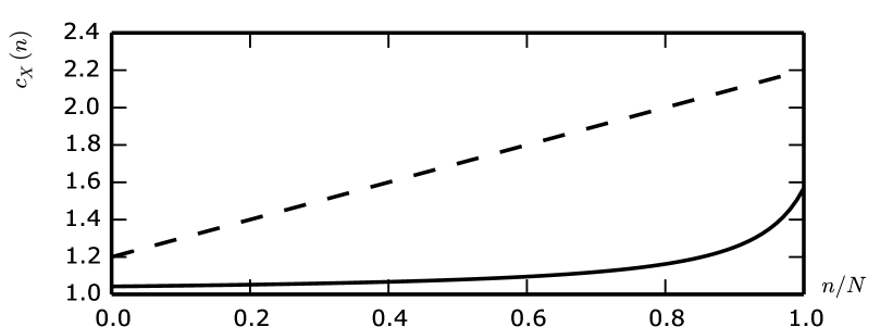
(a) Cost functions: $c_{A}(n)\triangleq 1.2+n/N$ (dashed line) and $c_{B}(n)\triangleq 1+(1.08-n/N)^{-1}/22$ (solid line).

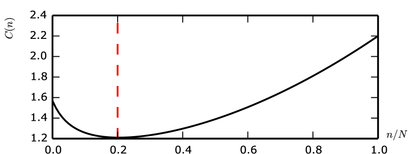
(b) One-step social cost as a function of the fraction of agents choosing action $A$. The dashed vertical line highlights the minimum at a population profile of $n^{*}/N=0.2$.

Figure 1: The setting of the running example. Despite the fact that the curves do not intersect, the optimum of the social cost is achieved when both actions are used – with a $0.2$-fraction of agents choosing action $A$.

The social cost $C(n^{A}_{t})$ scales the costs of the two actions at time $t$ with the proportions of agents taking the two actions, i.e.,

$$C(n^{A}_{t})\triangleq\frac{n^{A}_{t}}{N}\cdot c_{A}(n^{A}_{t})+\frac{n^{B}_{t}}{N}\cdot c_{B}(n^{B}_{t}).$$ (1)

The social cost corresponding to the cost functions of Figure 1(a) is shown in Figure 1(b). We also define the time-averaged social cost as follows:

$$\widehat{C}_{T}\triangleq\frac{1}{T}\sum_{t=1}^{T}C(n^{A}_{t}),$$ (2)

which will be used to illustrate the evolution of the social cost in simulations. The social optimum $n^{*}$ of the social cost $C$ is defined in the usual way:

$$n^{*}=\min_{n\in\{0,1,\ldots,N\}}\frac{n}{N}\cdot c_{A}(n)+\frac{N-n}{N}\cdot c_{B}(N-n).$$ (3)

Given this basic setting, we wish to control these various costs by influencing individual agents’ decisions. This is done using simple signalling schemes. We consider two specific schemes.

• The first one de-synchronises greedy agents with different actuation delays, i.e., delays between receiving a signal and taking a corresponding action.

• The second one de-synchronises agents with various levels of risk aversion.

We will later show that under reasonable assumptions on the behaviour of agents, these signalling schemes lead to desirable outcomes.

3 Related Work

Before proceeding, we now briefly mention some related work. Note that the related work spans many fields and an exhaustive survey is neither possible nor intended here.

Congestion problems are important in networking, control, operations research, and game theory [20, 9, 23, 12]. Our work proposes signalling solutions that reduce congestion by introducing a non-trivial amount of uncertainty through randomisation. Although it may seem surprising given the simplicity of the model, our results are unknown in the literature to the best of our knowledge.

In operations research and mathematical optimisation, congestion problems are often considered to be deterministic nonlinear resource allocation problems (e.g., [20, 9, 23, 12]). In our work, however, the decision-maker only chooses the signals to send, instead of an allocating the resources, per se.

Game theoretical models assume agents that act strategically, i.e., each agent has a non-negligible effect on the outcome. The study of one-shot congestion games has a long history, starting with [13]. The socially optimal and Nash equilibrium outcomes of congestion games have been compared in [14, 1], and [2]. These works show that when agents have full information, a resulting equilibrium outcome can incur much higher total congestion than a socially optimal outcome. An important distinction of our work is that, instead of a static game theoretical model, we consider a dynamic model evolving over time. The agents do not observe other agents’ actions, nor do they act strategically: the only information they have about the congestion of the resources is obtained from signals broadcast by a central agent. We model a heterogeneous population of agents, i.e., a large number of agents with a variety of fixed policies. These agents do not act strategically in the fashion of price-taking participants in large markets, which reflects situations where each agent has very limited impact on the outcome as a whole. We take the view of the central agent, who has perfect knowledge of the congestion across resources up to the previous time step, but imperfect knowledge of the stochastic composition of the population of users. Our goal is to minimise the social welfare or total congestion: we study how the amount of information withheld can contribute to better social outcomes. In contrast to evolutionary game theory, where agents of different types interact and the population profile (or distribution) evolves over time, the population profile remains fixed in our setting, and only the action profile evolve over time.

Our random signals are reminiscent of perturbation schemes in repeated games, such as Follow-the-Perturbed-Leader [6], trembling-hand equilibrium [19], stochastic fictitious play [7], or the power of two choices [11]. When the agents use such randomised algorithms in their decision-making, the resulting demand process has been shown to be behave rather well in theory (e.g., [11]), as well as in a number of applications, e.g., in parking [17], bike sharing [15], and charging electric vehicles [16]. However, we propose a signalling and guidance scheme that combines randomization and intervals.

In the transportation literature, [21] introduces the notion of equilibrium as the limit of the congestion distribution if it exists. [8] considers a number of notions of noisy signals and studies greedy policies and equilibria. Our approach is also related to signalling of parking space availability [18].

Our interval signalling scheme is reminiscent of the equilibrium outcome of [4] in the context of signalling games in economics (cf. [22] for an up-to-date survey). However, we consider the problem of optimal signalling in a dynamic system, whereas [4] considers Nash equilibrium signalling in single-shot games. For signalling games, [5] shows that more information does not generally improve the equilibrium welfare of agents. Their notion of “information,” due to [3], is however very different from ours.

Finally, let us note that there is also a related draft [10] by the present authors, which explores the notion of $r$-extreme interval signalling and optimisation over truthful interval signals.

4 Scalar Signalling

In this section, we model agents with different actuation delays – i.e., delays between receiving a signal and taking a corresponding action – and introduce a signalling scheme with the aim of desynchronising these agents.

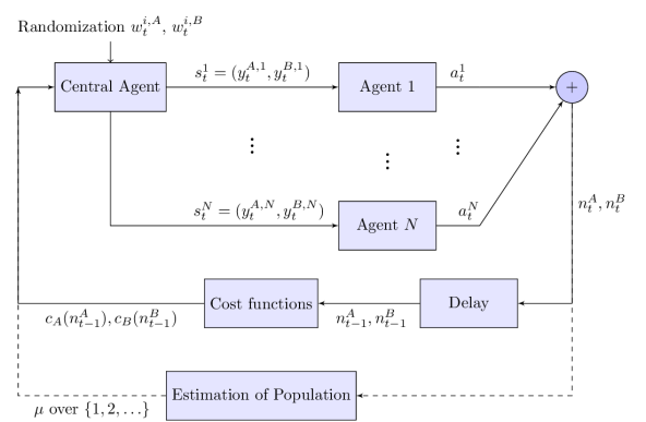
Figure 2: Block diagram for scalar signalling.

Notationwise, let $H_{t}$ denote the congestion costs at time $t$:

$$H_{t}\triangleq(c_{A}(n^{A}_{t}),c_{B}(n^{B}_{t}))\in\mathbb{R}^{2}.$$

We write $s^{i}_{t}\triangleq s^{i}_{t}(H_{t-1})$ denotes the signal that the central agent sends to agent $i$ at every time $t$. For a fixed integer $d$, a signalling scheme is a sequence of mappings

$$\{s^{i}_{t}:\mathbb{R}^{2}\to\mathbb{R}^{d}\mid i=1,\ldots,N,t=1,2,\ldots\}.$$ (4)

4.1 $\sigma$-Scalar Signalling

We propose the following scalar signalling scheme, which corresponds to the case $d=2$ in (4), with a parameter $\sigma>0$. At every time step $t$, the central agent sends to each agent $i$ a distinct signal $s^{i}_{t}:=(y^{A,i}_{t},y^{B,i}_{t})\in\mathbb{R}^{2}$:

$$y^{A,i}_{t} \triangleq c_{A}(n^{A}_{t-1})+w^{i,A}_{t},$$ (5)

$$y^{B,i}_{t} \triangleq c_{B}(n^{B}_{t-1})+w^{i,B}_{t},$$ (6)

where $\{(w^{i,A}_{t},w^{i,B}_{t}):i=1,\ldots,N;\;t=1,2,\ldots\}$ are independent and identically distributed (i.i.d. ) zero-mean normal random variables such that ${\mathbb{E}}(w^{i,A}_{t}-w^{i,B}_{t})^{2}=\sigma^{2}$ for all $i$ and $t$.

Remark 1 (Random Signals).

The signals $\{s^{i}_{t}\}$ in this section and the next are generated by the random variables – $\{w^{i,A}_{t},w^{i,B}_{t}\}$ in this section and $\{\nu_{t},\eta_{t}\}$ in the next. In the rest of the paper, all expectations and probabilities are with respect to the distribution of these random signals.

In contrast to signalling schemes that solve an allocation problem to minimise the social cost and coerce each agent towards its assigned action, $\sigma$-scalar signalling is scalar-truthful in the following sense:

$${\mathbb{E}}y^{A,i}_{t} =c_{A}(n^{A}_{t-1}),\quad\mbox{and}\quad{\mathbb{E}}y^{B,i}_{t}=c_{A}(n^{B}_{t-1}),$$

for all $i$ and $t$, where the expectation is over the random variables $\{w^{i,X}_{t}\}$. We will show in Section 4.3 that it is possible to reduce the social cost by setting the parameter $\sigma$ to a non-trivial value.

4.2 Agent Population and Policies

In response to the history of signals received prior to time $t$, every agent $i$ takes action $a_{t}^{i}$. We assume that every agent acts based only on the signals, without considering the response of other agents to its own action. This is a reasonable assumption for three reasons. First, it is hard for the agent to obtain more information than the signal sent by the central agent. Second, the agents know that the signals received are truthful. Finally, the environment may be rapidly changing, making independent decisions difficult.

Formally, let $S^{i}_{t}$ denote the history of signals received by agent $i$ up to time $t$: $S^{i}_{t}\triangleq\{s^{i}_{1},\ldots,s^{i}_{t-1}\}$. Let $\mathcal{S}_{t}$ denote the set of possible realisations of signal histories up to time $t$. A sequence of mappings from signal history to action, $\mathcal{S}_{t}\to\{A,B\}$ for $t=1,2,\ldots$, is called a policy.

We let $\Omega$ denote the set of all possible types of agents. We introduce a probability measure $\mu$ over the set $\Omega$, which describes the distribution of the population of agents into types. We assume that each type $\omega\in\Omega$ is associated with a policy, and every agent of type $\omega$ follows the policy $\pi^{\omega}:\mathcal{S}_{t}\to\{A,B\}$. For a population of $N$ agents, we assume that $\mu$ is such that $\mu(O)N$ is a non-negative integer for all $O\subseteq\Omega$. Consequently, $\mu(\omega)N$ denotes the number of agents with policy $\pi^{\omega}$. The following assumption simplifies the analysis.

Assumption 1.

The true distribution $\mu$ is known to the central agent.

It is also reasonable that the central agent is capable of estimating the distribution of agents $\mu$ using statistical estimation techniques. Estimating distribution of agents is possible by Bayesian or maximum a-posteriori methods. If the estimation is not accurate, the central agent can always fall back to sending no signal, which creates no more congestion than there already is.

4.2.1 $\pi^{k}$-policies

In the case of scalar signalling, we assume that the set of possible types is $\Omega=\{1,2,\ldots\}$. Each agent of type $k\in\Omega$ has an actuation delay of $k$ time steps, i.e., it acts at time $t$ upon the signal $s^{i}_{t-k}$ received at the time step $t-k$ – if the latter is defined. This effectively models the delay between when an agent makes the decision which action to take, and when it contributes to congestion. These delays do not come from communication, but from the agent-specific delay between making a decision and causing congestion. For example, a driver may decide to take route $A$ at time $t-k$, but begin the journey only at time $t$, resulting in the delay between deciding on a route and reaching a particular congested road segment. Another example is the computational delay between receiving stock market information and deciding to invest in a stock.

More precisely, in response to the scalar signalling scheme with parameter $\sigma$, i.e., $s^{i}_{t}:=(y^{A,i}_{t},y^{B,i}_{t})$, each agent $i$ of type $k$ acts according to the following policy $\pi^{k}$:

$$a_{t}^{i} =\pi^{k}(S^{i}_{t})=\pi^{k}(s^{i}_{t-k})$$

$$=\begin{cases}\arg\min_{X=A,B}\quad y^{X,i}_{t-k},&\quad\mbox{if }t\geqslant k+1,\\ A,&\quad\mbox{otherwise},\end{cases}$$ (7)

i.e., the agent chooses greedily the action with the smallest cost signal at time $t-k$.

4.3 Guarantees

In this section, we characterise the social cost resulting from $\sigma$-scalar signalling and a population of agents following policies $\{\pi^{k}:k=1,2,\ldots\}$. Furthermore, we show that the expected distribution of agents between the actions converges for every initial condition.

For clarity of exposition, we first consider a homogeneous population. We analyse the expected value and concentration property of the social cost, and show the convergence of each agent’s action profile. Our analysis methods can be used to obtain corresponding guarantees for the heterogeneous population cases. We also illustrate our main theoretical guarantees with simulations.

4.3.1 Homogeneous Population

In this section, we consider a homogeneous population of agents with the policy $\pi^{1}$, i.e., the case $\mu(1)=1$. In other words, we assume that every agent $i$ acts according to $\pi_{1}$.

First, we focus on the next-step outcome and establish closed-form expressions for the expectation of the number of agents taking action $A$.

Lemma 1 (Conditional Distribution of $n^{A}_{t}$).

Suppose that $n^{A}_{t-1}$ takes a fixed value $n\in\{1,\ldots,N\}$ and that all agents are of policy $\pi^{1}$. Consider an arbitrary time step $t>1$ and arbitrary $n^{A}_{t-1}$. Let $p_{\sigma,n}\triangleq\Phi_{\sigma}(c_{B}(N-n)-c_{A}(n))$. Then, we have

$${\mathbb{P}}(n^{A}_{t}=m\mid n^{A}_{t-1}=n)=\binom{N}{m}p_{\sigma,n}^{m}(1-p_{\sigma,n})^{N-m}.$$

Proof.

Recall that $y^{A,i}_{1}:=c_{A}(n^{A}_{t})+w_{i}$, and $y^{B,i}_{1}:=c_{B}(N-n^{A}_{t})+w_{i}$. Notice that $a_{t}^{i}$ is a random variable. The number of agents taking action $A$ at time $t$ is:

$$n^{A}_{t}= \sum_{i=1}^{N}1_{[a^{i}_{t}=A]}.$$

Clearly, for a fixed $t$, $\{w^{A}_{i,t}-w^{B}_{i,t}:i=1,\ldots,N\}$ is i.i.d. with normal distribution $N(0,\sigma^{2})$. Hence, for a fixed $t$, $\{1_{[a^{i}_{t}=A]}:i=1,\ldots,N\}$ are i.i.d. Bernoulli random variables, each with parameter ${\mathbb{P}}(a^{i}_{t}=A)$.

Let $\Phi_{\sigma}$ denote the tail probability function of the distribution $N(0,\sigma^{2})$. Observe that

$${\mathbb{P}}(a^{i}_{t}=A) ={\mathbb{P}}(y^{A,i}_{t}<y^{B,i}_{t})$$

$$={\mathbb{P}}(c_{A}(n^{A}_{t-1})+w^{A}_{i,t}<c_{B}(N-n^{A}_{t-1})+w^{B}_{i,t})$$

$$={\mathbb{P}}(w^{A}_{i,t}-w^{B}_{i,t}<c_{B}(N-n^{A}_{t-1})-c_{A}(n^{A}_{t-1}))$$

$$=\Phi_{\sigma}(c_{B}(N-n)-c_{A}(n))=p_{\sigma,n},$$

where we used the assumption that $n^{A}_{t-1}=n$.

Since $n^{A}_{t}$ is a sum of Bernoulli random variables, the claim follows by the binomial probability mass function. ∎

Next, we can derive a closed-form expression for the expectation of the next-step social cost.

Theorem 1 (Expected Next-step Social Cost).

Let us take the assumptions as in Lemma 1. For every parameter $\sigma>0$, and allocation $n\in\{1,\ldots,N\}$ to action $A$, we have

$$\frac{{\mathbb{E}}C(n^{A}_{t})}{C(n)}=\sum_{m=-\infty}^{\infty}\frac{C(m)}{C(n)}\binom{N}{m}p_{\sigma,n}^{m}(1-p_{\sigma,n})^{N-m},$$

where the expectation is conditioned on $n^{A}_{t-1}=n$.

Proof.

Observe that

$${\mathbb{E}}C(n^{A}_{t}) =\sum_{m=-\infty}^{\infty}C(m){\mathbb{P}}(n^{A}_{t}=m)$$

$$=\sum_{m=-\infty}^{\infty}C(m)\binom{N}{m}p_{\sigma,n^{*}}^{m}(1-p_{\sigma,n^{*}})^{N-m}.$$ (8)

The claim follows. ∎

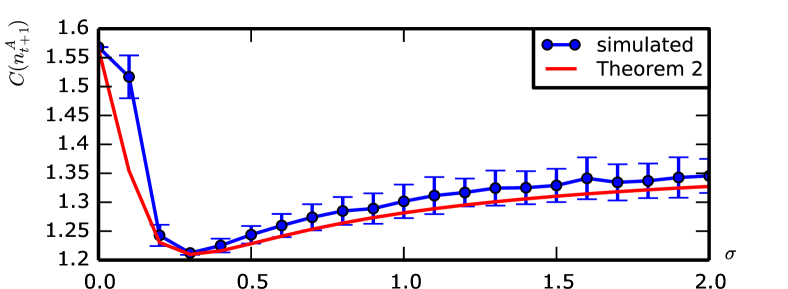
(a) Next-step social cost $C(n^{A}_{t})$ versus parameter $\sigma$ with $n^{A}_{t-1}=n^{*}$. Observe that the social cost is minimum at $\sigma=0.3$ and that the variance decreases as we approach the minimum.

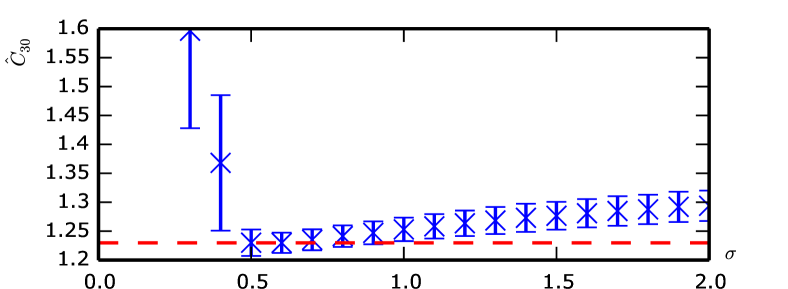
(b) Time-averaged social cost $\widehat{C}_{30}$ versus parameter $\sigma$ with $n^{A}_{1}=n^{*}$. The dashed horizontal line is at the unique optimum.

Figure 3: $\sigma$-scalar signalling, homogeneous population of $N=40$, and the cost functions of Figure 1(a).

Recall that $n^{*}$ denotes the socially optimal allocation of agents to action $A$. Figure 3(a) illustrates the expected social cost of Theorem 1 as a function of the parameter $\sigma$, along with the simulated mean and standard deviation of $C(n^{A}_{t})$. In particular, observe that by setting $\sigma=0.3$, the next-step social cost $C(n^{A}_{t})$ achieves the theoretical minimum social cost $C(n^{*})$ of Figure 3(a), provided that the population distribution is optimal at the current time step ($n_{t-1}^{A}=n^{*}$). Furthermore, Figure 3(b) shows the time-averaged social cost $\widehat{C}_{T}$ can achieve values close to the theoretical minimum social cost by setting the parameter $\sigma$ appropriately. Hence, $\sigma$-scalar signalling is useful even when we do not satisfy the condition $n_{t-1}^{A}=n^{*}$ for many time indices $t$.

Remark 2 (Optimal $\sigma$).

It is clear from Figure 3(a) and by substituting $p_{\sigma,n}\triangleq\Phi_{\sigma}(c_{B}(N-n)-c_{A}(n))$ into Theorem 1 that we can readily minimise the next-step expected social cost by optimising the amount of noise $\sigma$.

Next, we quantify the concentration of the social cost around its expected value, which is already hinted at in the error bars of Figure 3(a).

Theorem 2 (Concentration of Next-step Social Cost).

Suppose that the assumptions of Theorem 1 and that the functions $c_{A}$ and $c_{B}$ are Lipschitz with constant $L$. We have

$${\mathbb{P}}\left(\left\lvert\frac{C(n^{A}_{t})}{C(n^{*})}-\frac{{\mathbb{E}}C(n^{A}_{t})}{C(n^{*})}\right\rvert\geqslant\varepsilon\right)\leqslant 2\exp\left(-\frac{2\varepsilon^{2}C(n^{*})}{2(L+1)}\right),$$

where the probability is conditioned on $n^{A}_{t-1}=n^{*}$.

Proof.

Let

$$X_{i}=1_{[a^{i}_{t}=A]},\quad\mbox{for all }i=1,\ldots,N,$$

so that $n^{A}_{t}=\sum_{i}X_{i}$. Let $f$ be such that

$$f(X_{1},\ldots,X_{N})$$

$$=C(n^{A}_{t})/C(n^{*})$$

$$=\frac{1}{C(n^{*})}\Big{[}\frac{\sum_{i}X_{i}}{N}\cdot c_{A}\left(\frac{\sum_{i}X_{i}}{N}\right)$$

$$\quad\quad+\frac{N-\sum_{i}X_{i}}{N}\cdot c_{B}\left(\frac{N-\sum_{i}X_{i}}{N}\right)\Big{]}.$$

Let $x_{1},\ldots,x_{N},\widehat{x}_{i}\in\{0,1\}$. Observe that since $c_{A}$ and $c_{B}$ take values in $[0,1]$ and are $L$-Lipschitz by assumption, by simple algebra, we obtain

$$\sup\left\lvert f(x_{1},\ldots,x_{N})-f(x_{1},\ldots,\widehat{x}_{i},\ldots,x_{N})\right\rvert$$

$$\leqslant\frac{2(1/N+L/N)}{C(n^{*})},$$

for all $i$. Hence, by McDiarmid’s inequality, we obtain the claim. ∎

Next, we consider the normalised random process $n^{A}_{t}/N$ for $t=0,1,2,\ldots$ In particular, we consider the expectation of that process, i.e., the sequence

$$x^{i}_{t}\triangleq{\mathbb{P}}(a^{i}_{t}=A)={\mathbb{E}}\frac{n^{A}_{t}}{N},\quad t=1,2,\ldots$$

We show that this sequence converges. In order words, the action profile of every agent converges under $\sigma$-scalar signalling if every agent follows the $\pi^{1}$ policy (7).

Theorem 3 (Convergence).

Suppose that the assumptions of Theorem 1 hold. For every initial condition $x^{i}_{1}={\mathbb{P}}(a^{i}_{1}=A)$, the sequence $x^{i}_{t}={\mathbb{P}}(a^{i}_{t}=A)$ converges as $t\to\infty$.

Proof.

Observe that, for all $t>2$, we have

$$x^{i}_{t} ={\mathbb{P}}(a^{i}_{t}=A)$$ (9)

$$={\mathbb{P}}(w^{A}_{i,t}-w^{B}_{i,t}<c_{B}(N-n^{A}_{t-1})-c_{A}(n^{A}_{t-1}))$$ (10)

$$=\sum_{m}{\mathbb{P}}(w^{A}_{i,t}-w^{B}_{i,t}<c_{B}(N-m)-c_{A}(m)){\mathbb{P}}(n^{A}_{t-1}=m)$$ (11)

$$=\sum_{m}\Phi_{\sigma}(c_{B}(N-m)-c_{A}(m)){\mathbb{P}}(n^{A}_{t-1}=m),$$ (12)

where

$${\mathbb{P}}(n^{A}_{t-1}=m) =\binom{N}{m}{\mathbb{P}}(a^{i}_{t-1})^{m}(1-{\mathbb{P}}(a^{i}_{t-1}))^{N-m}$$ (13)

$$=\binom{N}{m}(x^{i}_{t-1})^{m}(1-x^{i}_{t-1})^{N-m}.$$ (14)

By combining (12) and (13), we obtain a function $f:\mathbb{R}\to\mathbb{R}$ that describes the iterated function process $\{x^{i}_{t}:t=1,2,\ldots\}$:

$$x^{i}_{t}=f(x^{i}_{t-1}),\quad\mbox{for all }t.$$

It is easy to verify that there exists an $\ell<1$ such that for all $x,y$,

$$\left\lvert f(x)-f(y)\right\rvert\leqslant\ell\left\lvert x-y\right\rvert.$$

Hence, $f$ is a contraction and the claim follows from Banach fixed-point theorem. ∎

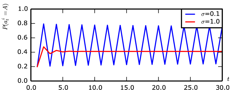
(a) Iterated function process $x^{i}_{t}$ for various values of $\sigma$.

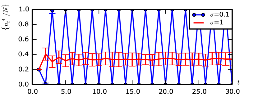
(b) The process $\{n^{A}_{t}/N\}$ over time.

Figure 4: $\sigma$-scalar signalling, homogeneous population of $N=40$, and the cost functions of Figure 1(a).

To illustrate Theorem 3, Figure 4(a) shows the process $x^{i}_{t}$ for various values of $\sigma$, whereas Figure 4(b) shows the related random process $\{n^{A}_{t}/N\}$. Observe that for the parameter value $\sigma=0.6$, the process $\{n^{A}_{t}/N\}$ converges to values close to the optimal population profile $n^{*}/N=0.2$ (cf. Figure 1(b)), whereas for other parameter values, we see flapping in the population profiles and values away from the optimum.

As a corollary of Theorem 3, we obtain the following.

Corollary 1.

The random processes $n_{t}^{A}/N$ and $C(n_{t}^{A})$ converge in distribution as $t\to\infty$.

Remark 3 (Limit of $C(n_{t}^{A})$).

It follows from Theorem 3 that the limit distribution of the random process $C(n_{t}^{A})$ depends on the parameter $\sigma$, which can be optimised.

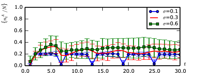
(a) The processes $\{n^{A}_{t}/N\}$ over time for a uniform population distribution $\mu$ over delays of $1,2,\ldots,5$.

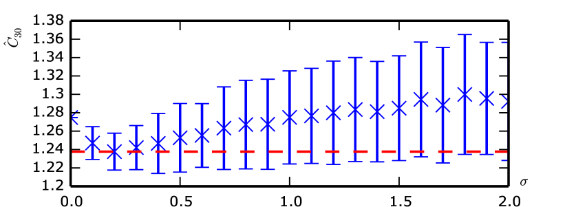
(b) The time-averaged social cost $\widehat{C}_{30}$ versus parameter $\sigma$ for uniform population distribution $\mu$ over delays of $1,2,\ldots,20$.

Figure 5: $\sigma$-scalar signalling on the cost functions of Figure 1(a) with $N=40$ agents.

4.3.2 Heterogeneous Population

In this section, we consider a distribution $\mu=(\mu_{1},\ldots,\mu_{K})$ of agents over the policies $\pi^{1},\ldots,\pi^{K}$, i.e., with $\mu_{j}N$ agents with delays $j$ for $j=1,\ldots,K$. We first derive the following analogue of Lemma 1.

Lemma 2 (Conditional Distribution of $n^{A}_{t}$).

Suppose that Assumption 1 holds. Consider an arbitrary time step $t>K$ and suppose that $n^{A}_{t-k}=n_{0}$ for all $k=1,\ldots,K$. Let $p_{\sigma}\triangleq\Phi_{\sigma}(c_{B}(N-n_{0})-c_{A}(n_{0}))$. Then, we have

$${\mathbb{P}}(n^{A}_{t}=m\mid n^{A}_{t-k}=n_{0}\mbox{ for }k=1,\ldots,K)$$

$$=\sum_{\left\lvert\alpha\right\rvert=m}\binom{m}{\alpha}\prod_{j=1}^{K}\binom{\mu_{j}N}{\alpha_{j}}p_{\sigma}^{\alpha_{j}}(1-p_{\sigma})^{\mu_{j}N-\alpha_{j}},$$

where $\alpha=(\alpha_{1},\ldots,\alpha_{K})$ denotes a multi-index.

Proof.

Let $n^{A}_{j,t}$ denote the number of agent of type $j$ who choose action $A$ at time $t$. By the same argument as Lemma 1, we have

$${\mathbb{P}}(n^{A}_{j,t}=m)=\binom{\mu_{j}N}{m}p_{\sigma}^{m}(1-p_{\sigma})^{\mu_{j}N-m},\quad j=1,\ldots,K.$$

By definition, we have

$${\mathbb{P}}(n^{A}_{t}=m) ={\mathbb{P}}\left(\sum_{j=1}^{K}n^{A}_{j,t}=m\right)$$

$$=\sum_{\left\lvert\alpha\right\rvert=m}\binom{m}{\alpha}{\mathbb{P}}(n^{A}_{1,t}=\alpha_{1})\ldots{\mathbb{P}}(n^{A}_{K,t}=\alpha_{K}).$$

The claim follows by algebra. ∎

Using Lemma 2, we can readily derive analogues of the expected next-step social cost (Theorem 1), the concentration of social cost (Theorem 2), and the convergence of action profiles (Theorem 3) guarantees for heterogeneous populations. Figures 5(a) illustrates the convergence of the population profile $n_{t}^{A}/N$ with a heterogeneous population under $\sigma$-scalar signalling. Observe that, as in Figure 4(b), a cyclic flapping behaviour is visible at low values of $\delta$, e.g., $\delta=0.1$.

An empirical study of the time-averaged social cost $\widehat{C}_{t}$ shows a dependence on the parameter $\sigma$ similar to the next-step social cost $C(n_{t}^{A})$, which can be seen by comparing Figure 5(b) to Figure 3(a).

5 Interval Signalling

In this section, we model agents with various levels of risk aversion, and present a broadcast signalling scheme that desynchronises them. Each signal is composed of pairs of endpoints, hence, the name interval signalling. The overall closed-loop system composed of the central agent and the agents is shown in Figure 6.

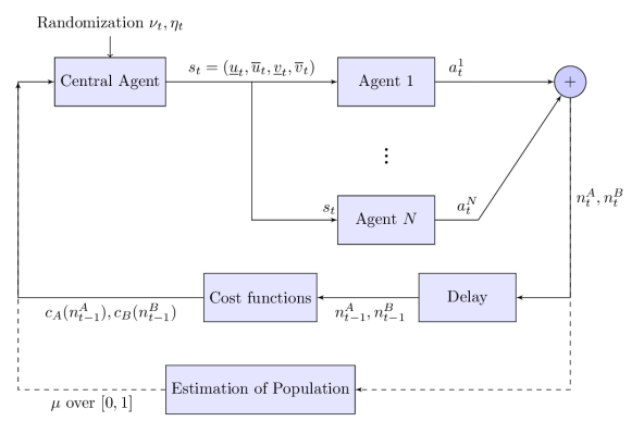
Figure 6: Block diagram for interval signalling.

5.1 $(\delta,\gamma)$-Interval signalling

In this section, we present a signalling scheme that broadcast the same signal to all agents. Let $\delta$ and $\gamma$ denote non-negative constants. In the $(\delta,\gamma)$-interval signalling scheme, a central agent broadcasts to all agents the same signal $s^{i}_{t}=s_{t}$ for all $i$. This is in constrast to $\sigma$-scalar signalling, where the central agent sends a distinct signal to every agent $i$. For every time step $t$, the signal $s_{t}=(\underline{u}^{A}_{t},\overline{u}^{A}_{t},\underline{u}^{B}_{t},\overline{u}^{B}_{t})\in\mathbb{R}^{4}$ is defined as follows:

$$\underline{u}^{A}_{t}\triangleq c_{A}(n^{A}_{t-1})+\nu_{t}-\delta/2,\quad \overline{u}^{A}_{t}\triangleq c_{A}(n^{A}_{t-1})+\nu_{t}+\delta/2,$$ (15)

$$\underline{u}^{B}_{t}\triangleq c_{B}(n^{B}_{t-1})+\eta_{t}-\gamma/2,\quad \overline{u}^{B}_{t}\triangleq c_{B}(n^{B}_{t-1})+\eta_{t}+\gamma/2.$$ (16)

where $\nu_{t}$ and $\eta_{t}$ are i.i.d. uniform random variables with supports:

$$\mbox{Supp}(\nu_{t}) =[-\delta/2,\delta/2],\quad\mbox{Supp}(\eta_{t})=[-\gamma/2,\gamma/2].$$

Figure 7 illustrates the interval $[\underline{u}^{A}_{t},\overline{u}^{A}_{t}]$.

Figure 7: An illustration of interval signalling.

By construction, it is clear that $(\delta,\gamma)$-interval signalling scheme has the following property, which we call interval-truthfulness:

$$c_{A}(n^{A}_{t-1}) \in[\underline{u}^{A,i}_{t},\overline{u}^{A,i}_{t}]\mbox{ and }c_{B}(n^{B}_{t-1})\in[\underline{u}^{B,i}_{t},\overline{u}^{B,i}_{t}]$$

with probability $1$ for all $i$ and $t$. We will show in Section 5.2 that it is also possible to pick the parameters $(\delta,\gamma)$ to reduce the social cost.

5.1.1 $\pi^{\lambda}$-policies

In the case of interval signalling, we consider a set of agent types $\Omega=[0,1]$, where the type captures a level of risk aversion. Recall that every agent receives the same interval signal $s_{t}:=(\underline{u}_{t},\overline{u}_{t},\underline{v}_{t},\overline{v}_{t})$. In response, we assume that each agent of type $\lambda$ follows the policy $\pi^{\lambda}$:

$$a_{t}^{i}=\pi^{\lambda}(S^{i}_{t})=\pi^{\lambda}(s_{t}):=\arg\min_{X\in\{A,B\}}\lambda\underline{u}^{X}_{t}+(1-\lambda)\overline{u}^{X}_{t}.$$ (17)

These policies naturally model a notion of risk aversion. Observe that for $\lambda=0$, policy $\pi^{0}$ models a risk-averse agent, who makes decisions based solely on upper endpoints $\overline{u}^{A}_{t}$ and $\overline{u}^{B}_{t}$ of the respective intervals. Similarly, $\pi^{1}$ and $\pi^{1/2}$ model risk-seeking and risk-neutral agents. Although the extremes may be rare, it seems plausible that people combine the optimistic and pessimistic views in this fashion. The following example illustrates these policies.

Example 1.

Suppose that at time $t=1$, we have $c_{A}(n^{A}_{1})=1$ and $c_{B}(n^{B}_{1})=1$. For $\delta=1,\gamma=0.5$, the interval signal $s_{2}:=(\underline{u}_{2},\overline{u}_{2},\underline{v}_{2},\overline{v}_{2})$ at time $2$, could take the realisation of $(0.5,1.5,0.8,1.3)$. The risk-seeking agent with $\lambda=1$ would pick $A$, whereas the risk-averse agent with $\lambda=0$ would pick $B$.

5.2 Guarantees

In this section, we consider $(\delta,\gamma)$-interval signalling and $\pi^{\lambda}$-policies. For signalling scheme that broadcasts the same signal to all agents, the outcome corresponding to homogeneous populations is trivial since all agents would pick the same action. Hence, we consider directly a heterogenous population over a set of types $[0,1]$ and a population distribution $\mu$.

First, we derive a lemma for the conditional probability of taking action $A$. The main result of this section is an expression to evaluate the expected next-step social cost for a $\mu$-heterogeneous population under $(\delta,\gamma)$-interval signalling.

Lemma 3 (Conditional Probability of Action $A$).

Let $F_{\delta,\gamma,n}(\lambda)\triangleq{\mathbb{P}}(\pi^{\lambda}(s_{t})=A\mid n^{A}_{t-1}=n)$ denote, for every $\lambda\in\Omega$, the probability of an agent with policy $\pi^{\lambda}$ choosing action $A$ conditioned on the realisation of the random variable $n^{A}_{t-1}$. We have

$$F_{\delta,\gamma,n}(\lambda) ={\mathbb{P}}(\nu_{t}+\eta_{t}>c_{A}(n)+\delta(1/2-\lambda)$$

$$\quad-c_{B}(N-n)-\gamma(1/2-\lambda)),$$

where $\nu_{t}$ and $\eta_{t}$ are independent uniform random variables with supports $[-\delta/2,\delta/2]$ and $[-\gamma/2,\gamma/2]$.

Proof.

For every $\lambda\in\Omega$, the probability of an agent with policy $\pi^{\lambda}$ choosing action $A$ is

$${\mathbb{P}}(\pi^{\lambda}(s_{t})=A)$$

$$={\mathbb{P}}(\lambda\underline{u}^{A}_{t}+(1-\lambda)\overline{u}^{A}_{t}<\lambda\underline{u}^{B}_{t}+(1-\lambda)\overline{u}^{B}_{t})$$

$$={\mathbb{P}}(c_{A}(n^{A}_{t-1})+\delta(1/2-\lambda)-c_{B}(N-n^{A}_{t-1})-\gamma(1/2-\lambda)$$

$$\quad<-\nu_{t}+\eta_{t}),$$

where the first equality follows by definition of the policy $\pi^{\lambda}$, and the second equality follows by the definition of $(\delta,\gamma)$-interval signalling and simple algebra. The claim follows from the fact that $-\nu_{t}$ has the same distribution as $\nu_{t}$ by definition. ∎

Theorem 4 (Expected Next-Step Social Cost).

Suppose that the assumptions of Lemma 3 hold with $n=n^{*}$. Let $p_{\delta,\gamma,n^{*}}\triangleq\int_{\lambda\in[0,1]}F_{\delta,\gamma,n^{*}}(\lambda)\mu(\mathrm{d}\lambda)$. We have

$$\frac{{\mathbb{E}}C(n^{A}_{t})}{C(n^{*})}=\sum_{m=-\infty}^{\infty}\frac{C(m)}{C(n^{*})}\binom{N}{m}p_{\delta,\gamma,n^{*}}^{m}(1-p_{\delta,\gamma,n^{*}})^{N-m}.$$

Proof.

By the definition $F_{\delta,\gamma,n^{*}}(\lambda)\triangleq{\mathbb{P}}(\pi^{\lambda}(s_{t})=A\mid n^{A}_{t-1}=n^{*})$, we have

$${\mathbb{P}}(n^{A}_{t}=m\mid n^{A}_{t-1}=n^{*})=\binom{N}{m}p_{\delta,\gamma,n^{*}}^{m}(1-p_{\delta,\gamma,n^{*}})^{N-m}.$$

The claim follows by the same argument as the proof of Theorem 1 – cf. (8). ∎

Figure 8 presents in heat-map form the dependence of the next-step social cost $C(n^{A}_{t+1})$ on the parameters $\delta$ and $\gamma$ of the interval signalling scheme. Clearly, the optimal $(\delta,\gamma)$-values are a non-trivial region bounded away from $0$ and $\infty$. The simulated next-step social cost $C(n^{A}_{t+1})$ on Figure 8(a) coincides with the expected value of $C(n^{A}_{t+1})$ computed using Theorem 4 on Figure 8(b).

Remark 4 (Concentration of $C(n^{A}_{t})/C(n^{*})$).

In the case of $(\delta,\gamma)$-interval signalling, the social cost ratio $C(n^{A}_{t})/C(n^{*})$ is concentrated around the mean in a similar fashion to Theorem 2.

5.3 Long-Run Behaviour

In this section, we study empirically the long-run behaviour of the state process $n_{t}^{A}/N$ under $(\delta,\gamma)$-interval signalling. Figure 9(a) shows the simulated the time evolution of $n_{t}^{A}/N$. As in Figure 4(b), a severe flapping effect is exhibited at a low value of $\delta$, e.g., $\delta=0.5$. For higher values of $\delta$, there are hints of convergence.

Figure 9(b) shows the dependence of the time-averaged social cost $\widehat{C}_{T}$ on one parameter $\delta$, with the other parameter fixed at $\gamma=0.2$. Observe that the dependence is similar to that exhibited in the case of $\sigma$-scalar signalling (cf. 3(a)); moreover, at the optimal value of the parameter $\delta$, the social cost – although random – is close to the theoretical minimum (cf. 1(b)).

(a) Simulated next-step social cost $C(n^{A}_{t+1})$ versus $\delta$ and $\gamma$.

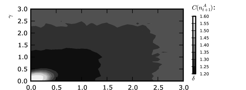
(b) Expected $C(n^{A}_{t+1})$ computed using Theorem 4 as a function of $\delta$ and $\gamma$

Figure 8: $(\delta,\gamma)$-interval signalling, cost functions of Figure 1(a), and heterogeneous population with $N=40$ and $\mu$ uniform over $\{1/N,\ldots,1\}$.

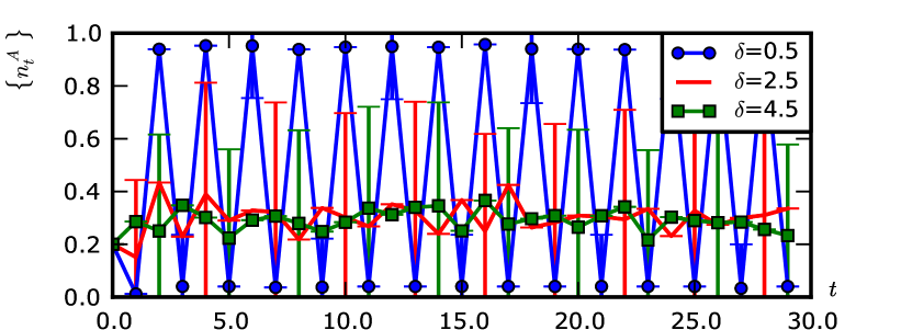
(a) The processes $\{n^{A}_{t}/N\}$ over time for $N=40$ agents, $\delta=0.1$, and $\gamma=0.2$.

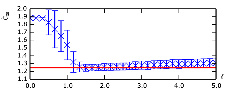
(b) Time-averaged social cost $\widehat{C}_{30}$ versus $\delta$ for a fixed $\gamma=0.2$, uniform distribution $\mu$ over $[0,1]$, and $N=40$. The dashed horizontal line is at the optimal $\delta$.

Figure 9: $(\delta,\gamma)$-interval signalling on the cost functions of Figure 1(a)

6 Conclusion

Our analysis and simulations give quantitative guidance on how to design signalling schemes in order to reduce the social cost. In particular, if we can estimate the true population mixture, e.g., using statistical estimation techniques, then we can optimise the signalling scheme to minimise the social cost. Although our analysis focuses on a congestion problem with two resources, the results can be extended to an arbitrary number of resources, e.g., by replacing the binomial distributions by a multinomial distribution in the analysis.

In contrast to signals that report past outcomes as deterministic numbers, which correspond to singular probability distributions, we propose random signals with non-singular distributions. When agents mistake deterministic signals for precise predictions of the future, their actions lead to the cyclic flapping behaviour. We show that agents who receive random signals with non-singular distributions exhibit cyclic behaviour to a lesser degree, which can improve the social cost.

Regarding future work, we pose several new questions that can be studied by extending our model. What happens when population size and composition change over time? This can be modeled by a Markovian sequence of random variables corresponding to agent types. How do the optimal parameter values for $\sigma,\delta,\gamma$ depend on those changes? This can be done by employing state-space control techniques to obtain these optimal values. Would our results hold if every agent had a distinct cost function, so as to model the priority given to some agents, e.g., when evacuating the young and elderly? This requires a new notion of consistency or truthfulness that is specialised to individual agents, as well as a new analysis.

References

- [1] E. Anshelevich, A. Dasgupta, J. Kleinberg, and E. Tardos. The price of stability for network design with fair cost allocation. In Foundations of Computer Science, 2004.
- [2] M.-F. Balcan, A. Blum, and Y. Mansour. The price of uncertainty. In Electronic Commerce, 2009.
- [3] D. Blackwell. Comparison of experiments. In J. Neymann, editor, Proceedings of the Second Berkeley Symposium on Mathematical Statistics and Probability, pages 93–102, 1951.
- [4] V. P. Crawford and J. Sobel. Strategic information transmission. Econometrica, 50(6):1431–1451, 1982.
- [5] J. R. Green and N. L. Stokey. A two-person game of information transmission. Journal of Economic Theory, 135(1):90 – 104, 2007.
- [6] J. Hannan. Approximation to Bayes risk in repeated play. In Contributions to the Theory of Games, volume 3, pages 97–139. Princeton University Press, 1957.
- [7] J. C. Harsanyi. Games with randomly disturbed payoffs: A new rationale for mixed-strategy equilibrium points. International Journal of Game Theory, 2(1):1–23, 1973.
- [8] J. L. Horowitz. The stability of stochastic equilibrium in a two-link transportation network. Transportation Research Part B: Methodological, 18(1):13–28, 1984.
- [9] T. Ibaraki and N. Katoh. Resource Allocation Problems: Algorithmic Approaches. MIT Press series in the foundations of computing. Mit Press, 1988.
- [10] J. Marecek, R. Shorten, and J. Y. Yu. Congestion management by interval signaling. CoRR, abs/1404.2458, 2014.
- [11] M. Mitzenmacher. The power of two choices in randomized load balancing. Parallel and Distributed Systems, IEEE Transactions on, 12(10):1094–1104, Oct 2001.
- [12] M. Patriksson. A survey on the continuous nonlinear resource allocation problem. European Journal of Operational Research, 185(1):1–46, 2008.
- [13] R. W. Rosenthal. A class of games possessing pure-strategy nash equilibria. International Journal of Game Theory, 2(1):65–67, 1973.
- [14] T. Roughgarden and E. Tardos. How bad is selfish routing? Journal of the ACM, 49(2):236–259, 2002.
- [15] A. Schlote, B. Chen, and R. Shorten. On closed-loop bicycle availability prediction. Intelligent Transportation Systems, IEEE Transactions on, PP(99):1–7, 2014.
- [16] A. Schlote, F. Hausler, T. Hecker, A. Bergmann, E. Crisostomi, I. Radusch, and R. Shorten. Cooperative regulation and trading of emissions using plug-in hybrid vehicles. Intelligent Transportation Systems, IEEE Transactions on, 14(4):1572–1585, Dec 2013.
- [17] A. Schlote, C. King, E. Crisostomi, and R. Shorten. Delay-tolerant stochastic algorithms for parking space assignment. Intelligent Transportation Systems, IEEE Transactions on, 15(5):1922–1935, Oct 2014.
- [18] A. Schlote, C. King, E. Crisostomi, and R. Shorten. Delay-tolerant stochastic algorithms for parking space assignment. Intelligent Transportation Systems, IEEE Transactions on, 15(5):1922–1935, Oct 2014.
- [19] R. Selten. Reexamination of the perfectness concept for equilibrium points in extensive games. International Journal of Game Theory, 4(1):25–55, 1975.
- [20] Y. Sheffi. Urban transportation networks: equilibrium analysis with mathematical programming methods. 1985.
- [21] M. Smith. The existence, uniqueness and stability of traffic equilibria. Transportation Research Part B: Methodological, 13(4):295–304, 1979.
- [22] J. Sobel. Giving and receiving advice. In D. Acemoglu, M. Arellano, and E. Dekel, editors, Advances in Economics and Econometrics, 2013.
- [23] S. M. Stefanov. Separable Programming: Theory and Methods. Applied Optimization. Springer, 2001.