Direct Density-Derivative Estimation and Its Application in KL-Divergence Approximation

Abstract

Estimation of density derivatives is a versatile tool in statistical data analysis. A naive approach is to first estimate the density and then compute its derivative. However, such a two-step approach does not work well because a good density estimator does not necessarily mean a good density-derivative estimator. In this paper, we give a direct method to approximate the density derivative without estimating the density itself. Our proposed estimator allows analytic and computationally efficient approximation of multi-dimensional high-order density derivatives, with the ability that all hyper-parameters can be chosen objectively by cross-validation. We further show that the proposed density-derivative estimator is useful in improving the accuracy of non-parametric KL-divergence estimation via metric learning. The practical superiority of the proposed method is experimentally demonstrated in change detection and feature selection.

1 Introduction

Derivatives of probability density functions play key roles in various statistical data analysis. For example:

• Mean shift clustering seeks modes of the data densities [1, 2, 3, 4], where the first-order density derivative is the key ingredient.

• The optimal bandwidth of kernel density estimation depends on the second-order density derivative [5].

• The bias of nearest-neighbor Kullback-Leibler divergence estimation is governed by the second-order density derivative [6].

• More applications in statistical problems such as regression, Fisher information estimation, parameter estimation, and hypothesis testing are discussed in [7].

Given such a wide range of applications, accurately estimating the density derivatives from data has been a challenging research topic in statistics and machine learning.

A naive approach to density-derivative estimation from samples $\{x_{i}\}_{i=1}^{n}$ following probability density $p(x)$ on $\mathbb{R}$ is to perform density estimation and then compute its derivatives. For example, suppose that kernel density estimation (KDE) is used for density estimation:

$$\widehat{p}(x)\propto\sum_{i=1}^{n}K\left(\frac{x-x_{i}}{h}\right),$$

where $K$ is a kernel function (such as the Gaussian kernel) and $h>0$ is the bandwidth. Then the first-order density derivative is estimated as follows [8, 9]:

$$\widehat{p}^{\prime}(x)\propto\sum_{i=1}^{n}K^{\prime}\left(\frac{x-x_{i}}{h}\right).$$

A cross-validation method for selecting the bandwidth $h$ was proposed in [10]. However, since a good density estimator is not always a good density-derivative estimator, this approach is not necessarily reliable; this problem becomes more critical if higher-order density derivatives are estimated:

$$\widehat{p}^{(j)}(x)\propto\sum_{i=1}^{n}K^{(j)}\left(\frac{x-x_{i}}{h}\right).$$

A more direct approach of performing kernel density estimation for density derivatives was proposed [11]:

$$\widehat{p}^{(j)}(x)\propto\sum_{i=1}^{n}K\left(\frac{x-x_{i}}{h}\right).$$

However, this method suffers the bandwidth selection problem because the optimal bandwidth depends on higher-order derivatives than the estimated one [12].

In this paper, we propose a novel density-derivative estimator which finds the minimizer of the mean integrated square error (MISE) to the true density-derivative. The proposed method, which we call MISE for derivatives (MISED), possesses various useful properties:

• Density derivatives are directly estimated without going through density estimation.

• The solution can be computed analytically and efficiently.

• All tuning parameters can be objectively optimized by cross-validation.

• Multi-dimensional density derivatives can be directly estimated.

• Higher-order density derivatives can be directly estimated.

Through experiments on change detection and feature selection, we demonstrate the usefulness of the proposed MISED method.

2 Direct Density-Derivative Estimation

In this section, we describe our proposed MISED method.

2.1 Problem Formulation

Suppose that independent and identically distributed samples $\mathcal{X}=\{\boldsymbol{x}_{i}\}_{i=1}^{n}$ from unknown density $p(\boldsymbol{x})$ on $\mathbb{R}^{d}$ are available. Our goal is to estimate the $k$-th order (partial) derivative of $p(\boldsymbol{x})$,

$$p_{k,\boldsymbol{j}}(\boldsymbol{x})=\frac{\partial^{k}}{\partial x_{1}^{j_{1}}\partial x_{2}^{j_{2}}\dots\partial x_{d}^{j_{d}}}p(\boldsymbol{x}),$$ (1)

where $j_{1}+j_{2}+\dots+j_{d}=k$ for $j_{i}\in\{0,1,\dots,k\}$ and $\boldsymbol{j}=(j_{1},j_{2},\dots,j_{d})$. When $k=1$ (or $k=2$), $p_{k,\boldsymbol{j}}(\boldsymbol{x})$ corresponds to a single element in the gradient vector (or the Hessian matrix) of $p(\boldsymbol{x})$.

2.2 MISE for Density Derivatives

Let $g_{k,\boldsymbol{j}}(\boldsymbol{x})$ be a model of $p_{k,\boldsymbol{j}}(\boldsymbol{x})$ (its specific form will be introduced later). We learn $g_{k,\boldsymbol{j}}(\boldsymbol{x})$ to minimize the MISE to $p_{k,\boldsymbol{j}}(\boldsymbol{x})$:

$$J_{\boldsymbol{j}}(g_{k,\boldsymbol{j}}) =\int\left\{g_{k,\boldsymbol{j}}(\boldsymbol{x})-p_{k,\boldsymbol{j}}(\boldsymbol{x})\right\}^{2}\mathrm{d}\boldsymbol{x}$$

$$=\int\left\{g_{k,\boldsymbol{j}}(\boldsymbol{x})\right\}^{2}\mathrm{d}\boldsymbol{x}-2\int g_{k,\boldsymbol{j}}(\boldsymbol{x})p_{k,\boldsymbol{j}}(\boldsymbol{x})\mathrm{d}\boldsymbol{x}+\underbrace{\int\left\{p_{k,\boldsymbol{j}}(\boldsymbol{x})\right\}^{2}\mathrm{d}\boldsymbol{x}}_{C},$$ (2)

where $C$ is constant irrelevant to $g_{k,\boldsymbol{j}}(\boldsymbol{x})$ and thus can be safely ignored.

The first term in (2) is accessible since $g_{k,\boldsymbol{j}}(\boldsymbol{x})$ is a model specified by the user. The second term in (2) seems intractable at a glance, but integration by parts allows us to transform it as

$$\int g_{k,\boldsymbol{j}}(\boldsymbol{x})p_{k,\boldsymbol{j}}(\boldsymbol{x})\mathrm{d}\boldsymbol{x} =\int g_{k,\boldsymbol{j}}(\boldsymbol{x})\frac{\partial^{k}}{\partial x_{1}^{j_{1}}\partial x_{2}^{j_{2}}\dots\partial x_{d}^{j_{d}}}p(\boldsymbol{x})\mathrm{d}\boldsymbol{x},$$

$$=\int\left[g_{k,\boldsymbol{j}}(\boldsymbol{x})\frac{\partial^{k-1}}{\partial x_{1}^{j_{1}-1}\partial x_{2}^{j_{2}}\dots\partial x_{d}^{j_{d}}}p(\boldsymbol{x})\right]_{x_{1}=-\infty}^{x_{1}=\infty}\mathrm{d}\boldsymbol{x}_{\setminus x_{1}}$$

$$\phantom{=}-\int\frac{\partial}{\partial x_{1}}g_{k,\boldsymbol{j}}(\boldsymbol{x})\frac{\partial^{k-1}}{\partial x_{1}^{j_{1}-1}\partial x_{2}^{j_{2}}\dots\partial x_{d}^{j_{d}}}p(\boldsymbol{x})\mathrm{d}\boldsymbol{x},$$

where $\mathrm{d}\boldsymbol{x}_{\setminus x_{1}}$ denotes the integration except for $x_{1}$. The first term in the last equation vanishes under a mild assumption on the tails of $g_{k,\boldsymbol{j}}(\boldsymbol{x})$ and $\frac{\partial^{k-1}}{\partial x_{1}^{j_{1}-1}\partial x_{2}^{j_{2}}\dots\partial x_{d}^{j_{d}}}p(\boldsymbol{x})$. By repeatedly applying integration by parts $k$ times, we arrive at

$$J_{\boldsymbol{j}}(g_{k,\boldsymbol{j}}) =\int\left\{g_{k,\boldsymbol{j}}(\boldsymbol{x})\right\}^{2}\mathrm{d}\boldsymbol{x}-2(-1)^{k}\int\left\{\frac{\partial^{k}}{\partial x_{1}^{j_{1}}\partial x_{2}^{j_{2}}\dots\partial x_{d}^{j_{d}}}g_{k,\boldsymbol{j}}(\boldsymbol{x})\right\}p(\boldsymbol{x})\mathrm{d}\boldsymbol{x}+C.$$

Ignoring the constant $C$ and approximating the expectation by the sample average gives

$$\int\left\{g_{k,\boldsymbol{j}}(\boldsymbol{x})\right\}^{2}\mathrm{d}\boldsymbol{x}-\frac{2(-1)^{k}}{n}\sum_{i=1}^{n}\frac{\partial^{k}}{\partial x_{1}^{j_{1}}\partial x_{2}^{j_{2}}\dots\partial x_{d}^{j_{d}}}g_{k,\boldsymbol{j}}(\boldsymbol{x}_{i}).$$ (3)

2.3 Analytic Solution for Gaussian Kernels

As a density-derivative model $g_{k,\boldsymbol{j}}$, we use the Gaussian kernel model:

$$g_{k,\boldsymbol{j}}(\boldsymbol{x}) =\sum_{i=1}^{n}\theta_{\boldsymbol{j},i}\underbrace{\exp\left(-\frac{\|\boldsymbol{x}-\boldsymbol{x}_{i}\|^{2}}{2\sigma^{2}}\right)}_{\psi_{i}(x)}=\boldsymbol{\theta}_{\boldsymbol{j}}^{\top}\boldsymbol{\psi}(x),$$

for which the $k$-th derivative is given by

$$\frac{\partial^{k}}{\partial x_{1}^{j_{1}}\partial x_{2}^{j_{2}}\dots\partial x_{d}^{j_{d}}}g_{k,\boldsymbol{j}}(\boldsymbol{x}) =\sum_{i=1}^{n}\theta_{\boldsymbol{j},i}\underbrace{\frac{\partial^{k}}{\partial x_{1}^{j_{1}}\partial x_{2}^{j_{2}}\dots\partial x_{d}^{j_{d}}}\exp\left(-\frac{\|\boldsymbol{x}-\boldsymbol{x}_{i}\|^{2}}{2\sigma^{2}}\right)}_{\varphi_{\boldsymbol{j},i}(\boldsymbol{x})}=\boldsymbol{\theta}_{\boldsymbol{j}}^{\top}\boldsymbol{\varphi}_{\boldsymbol{j}}(x).$$

Substituting these formulas into the objective function (3) and adding the $\ell_{2}$-regularizer, we obtain a practical objective function:

$$\widetilde{J}_{\boldsymbol{j}}(\boldsymbol{\theta_{j}})=\boldsymbol{\theta}_{\boldsymbol{j}}^{\top}\mathbf{G}\boldsymbol{\theta_{j}}-2(-1)^{k}\boldsymbol{\theta_{j}}^{\top}\boldsymbol{h_{j}}+\lambda\boldsymbol{\theta_{j}}^{\top}\boldsymbol{\theta_{j}},$$ (4)

where

$$[\mathbf{G}]_{ij} =\int\psi_{i}(\boldsymbol{x})\psi_{j}(\boldsymbol{x})\mathrm{d}\boldsymbol{x}=(\pi\sigma^{2})^{d/2}\exp\left(-\frac{\|\boldsymbol{x}_{i}-\boldsymbol{x}_{j}\|^{2}}{4\sigma^{2}}\right)\quad\mbox{and}\quad\boldsymbol{h}_{\boldsymbol{j}}=\frac{1}{n}\sum_{i=1}^{n}\boldsymbol{\varphi}_{\boldsymbol{j}}(\boldsymbol{x}_{i}).$$

The minimizer of (4) is given analytically as

$$\widehat{\boldsymbol{\theta}}_{\boldsymbol{j}}=\arg\min_{\boldsymbol{\theta_{j}}}\widetilde{J}_{\boldsymbol{j}}(\boldsymbol{\theta_{j}})=(-1)^{k}\left(\mathbf{G}^{-1}+\lambda\mathbf{I}\right)\boldsymbol{h}_{\boldsymbol{j}},$$ (5)

where $\mathbf{I}$ denotes the identity matrix. Finally, a density-derivative estimator is obtained as

$$\widehat{g}_{k,\boldsymbol{j}}(\boldsymbol{x}) =\widehat{\boldsymbol{\theta}}_{\boldsymbol{j}}^{\top}\boldsymbol{\psi}(x).$$

We call this method the mean integrated square error for derivatives (MISED) estimator, which can be regarded as an extension of score matching for density estimation [13], least-squares density-difference for density-difference estimation [14, 15], and least-squares log-density gradients for log-density gradient estimation [4] to higher-order derivatives.

2.4 Model Selection by Cross-Validation

The performance of the MISED method depends on the choice of model parameters (the Gaussian width $\sigma$ and the regularization $\lambda$ in the current setup). Below, we describe a method to optimize the model by cross-validation, which essentially follows the same line as [10] for kernel density estimation:

1. Divide the sample $\mathcal{X}=\{\boldsymbol{x}_{i}\}_{i=1}^{n}$ into $T$ disjoint subsets $\{\mathcal{X}_{t}\}_{t=1}^{T}$.

2. The estimator $\widehat{g}^{(t)}_{k,\boldsymbol{j}}(\boldsymbol{x})$ is obtained using $\mathcal{X}\setminus\mathcal{X}_{t}$, and then the hold-out MISE to $\mathcal{X}_{t}$ is computed as

   $$\text{CV}(t) =\int\widehat{g}^{(t)}_{k,\boldsymbol{j}}(\boldsymbol{x})\mathrm{d}\boldsymbol{x}-\frac{2(-1)^{k}}{|\mathcal{X}_{t}|}\sum_{\boldsymbol{x}\in\mathcal{X}_{t}}\frac{\partial^{k}}{\partial x_{1}^{j_{1}}\partial x_{2}^{j_{2}}\cdots\partial x_{d}^{j_{d}}}\widehat{g}^{(t)}_{k,\boldsymbol{j}}(\boldsymbol{x}),$$ (6)

   where $|\mathcal{X}_{t}|$ denotes the number of elements in $\mathcal{X}_{t}$.

3. The model that minimizes $\text{CV}=\frac{1}{T}\sum_{t=1}^{T}\text{CV}(t)$ is chosen.

2.5 Numerical Examples

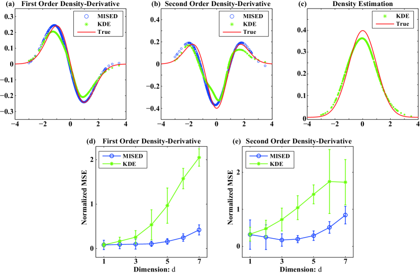
Figure 1: Estimation of the derivatives of the standard normal distribution. (a) and (b): First-order and second-order derivative estimation. (c): Density estimation (only by KDE). (d) and (e): Normalized mean squared error (MSE) for first-order and second-order derivative estimation as functions of the dimensionality of data.

Let us illustrate the behavior of MISED using $n=500$ samples drawn from the standard normal distribution. The Gaussian bandwidth $\sigma$ and the regularization parameter $\lambda$ included in MISED are chosen by 5-fold cross-validation from the nine candidates, $\sigma\in\left\{10^{-0.3},10^{-0.1375},\dots,10^{1}\right\}$ and $\lambda\in\{10^{-1},10^{-0.75},\ldots,10^{1}\}$. For comparison, we also test the Gaussian KDE where the Gaussian bandwidth $h$ is also chosen from the same candidate values by 5-fold cross-validation to minimize the hold-out MISE (6).

Figures 1 (a) and (b) depict the estimation results of the first-order and second-order density derivatives. The derivatives estimated by KDE are less accurate than MISED in particular for the second-order derivative, although the density itself is reasonably approximated as shown in Figure 1 (c). This result substantiates that a good density estimator is not necessary a good density-derivative estimator.

Next, we evaluate how the performance is affected when the dimensionality of the standard normal distribution is increased. We use the common $\sigma$ (and $\lambda$ for MISED) for all $\boldsymbol{j}$ and the summation of the hold-out MISE for all $\boldsymbol{j}$ is used as the cross-validation score. Figures 1 (d) and (e) show that the increase of the normalized mean squared errors (MSE) for the MISED method is much milder than that for KDE, illustrating the high reliability of MISED in high-dimensional problems.

3 Application to Kullback-Leibler (KL) Divergence Approximation

In this section, we apply density-derivative estimation to KL-divergence approximation.

3.1 Nearest-Neighbor KL-Divergence Approximation

The KL-divergence from one density $p_{1}(\boldsymbol{x})$ to another density $p_{2}(\boldsymbol{x})$, defined as

$$\mathrm{KL}(p_{1}\|p_{2})=\int p_{1}(\boldsymbol{x})\log\frac{p_{1}(\boldsymbol{x})}{p_{2}(\boldsymbol{x})}\mathrm{d}\boldsymbol{x},$$

is useful for various purposes such as two-sample homogeneity testing [16], feature selection [17], and change detection [18]. Here, we consider the KL-divergence approximator based on nearest-neighbor density estimation (NNDE) [19] from two sets of samples $\mathcal{X}_{1}=\{\boldsymbol{x}_{i}\}_{i=1}^{n_{1}}$ and $\mathcal{X}_{2}=\{\boldsymbol{x}_{i}\}_{i=n_{1}+1}^{n_{1}+n_{2}}$ following $p_{1}(\boldsymbol{x})$ and $p_{2}(\boldsymbol{x})$ on $\mathbb{R}^{d}$:

$$\widehat{\mathrm{KL}}(p_{1}\|p_{2})=\frac{1}{n_{1}}\sum_{i=1}^{n_{1}}\log\frac{(n_{1}-1)\mathrm{dist}_{1}(\boldsymbol{x}_{i})^{d}}{n_{2}\mathrm{dist}_{2}(\boldsymbol{x}_{i})^{d}},$$

where $\mathrm{dist}_{1}(\boldsymbol{x})$ and $\mathrm{dist}_{2}(\boldsymbol{x})$ denote the distance from $\boldsymbol{x}$ to the nearest samples in $\mathcal{X}_{1}$ and $\mathcal{X}_{2}$, respectively.

3.2 Metric Learning for NNDE-Based KL-Divergence Approximation

Although the KL-divergence itself is metric-invariant, the NNDE-based KL-divergence approximator is metric-dependent. Indeed, it was shown in [6] that the bias of the NNDE-based KL-divergence approximator at $\boldsymbol{x}$ is approximately proportional to

$$\frac{\text{tr}(\nabla\nabla p_{1})}{((n_{1}-1)p_{1})^{2/d}p_{1}}-\frac{\text{tr}(\nabla\nabla p_{2})}{(n_{2}p_{2})^{2/d}p_{2}},$$

where $\nabla\nabla p_{1}$ and $\nabla\nabla p_{2}$ are the Hessian matrices which are metric-dependent. Therefore, changing the metric in the input space is expected to reduce the bias.

It was shown in [6] that the best local Mahalanobis metric $(\boldsymbol{x}-\boldsymbol{x}^{\prime})^{\top}\widehat{\mathbf{A}}(\boldsymbol{x}-\boldsymbol{x}^{\prime})$ for point $\boldsymbol{x}$ that minimizes the above approximate bias is given by

$$\widehat{\mathbf{A}}\propto\left[\begin{array}[]{cc}\mathbf{U}_{+}&\mathbf{U}_{-}\\ \end{array}\right]\left(\begin{array}[]{cc}d_{+}\Lambda_{+}&0\\ 0&-d_{-}\Lambda_{-}\\ \end{array}\right)\left[\begin{array}[]{cc}\mathbf{U}_{+}&\mathbf{U}_{-}\\ \end{array}\right]^{\top},$$

where $\Lambda_{+}\in\mathbb{R}^{d_{+}\times d_{+}}$ and $\Lambda_{-}\in\mathbb{R}^{d_{-}\times d_{-}}$ are the diagonal matrices containing $d_{+}$ positive and $d_{-}$ negative eigenvalues of $\mathbf{B}$, respectively:

$$\mathbf{B} =\frac{1}{((n_{1}-1)p_{1})^{2/d}}\frac{\nabla\nabla p_{1}}{p_{1}}-\frac{1}{(n_{2}p_{2})^{2/d}}\frac{\nabla\nabla p_{2}}{p_{2}}.$$

The matrices $\widehat{\mathbf{A}}$ and $\mathbf{B}$ share the same eigenvectors, and $\mathbf{U}_{+}\in\mathbb{R}^{d\times d_{+}}$ and $\mathbf{U}_{-}\in\mathbb{R}^{d_{-}\times d_{-}}$ are collections of eigenvectors that correspond to the eigenvalues in $\Lambda_{+}$ and $\Lambda_{-}$, respectively.

In [6], the authors assumed that $p_{1}$ and $p_{2}$ are both nearly Gaussian, and estimated densities $p_{1}$ and $p_{2}$ as well as their Hessian matrices $\nabla\nabla p_{1}$ and $\nabla\nabla p_{2}$ from the Gaussian models with maximum likelihood estimation. It was demonstrated that the accuracy of NNDE-based KL-divergence approximation is significantly improved when $p_{1}$ and $p_{2}$ are nearly Gaussian.

3.3 Applying MISED to Metric Learning for NNDE-Based KL-Divergence Approximation

However, the above method does not work well if $p_{1}$ and $p_{2}$ are apart from Gaussian. Here, we propose to use our non-parametric density-derivative estimator in metric learning for NNDE-based KL-divergence approximation.

Since the scale of $\mathbf{B}$ is arbitrary, let us use the following rescaled matrix $\widetilde{\mathbf{B}}$ instead:

$$\widetilde{\mathbf{B}} =\frac{1}{(n_{1}-1)^{2/d}}\left\{\frac{p_{2}}{p_{1}}\right\}^{2/d+1}\nabla\nabla p_{1}-\frac{1}{n_{2}^{2/d}}\nabla\nabla p_{2}.$$ (7)

We estimate the Hessian matrices $\nabla\nabla p_{1}$ and $\nabla\nabla p_{2}$ by the proposed MISED method, and the density ratio $p_{2}/p_{1}$ by the unconstrained least-squares density-ratio estimator [20] that directly estimates the density ratio in a non-parametric manner without estimating each density. By this, we can perform metric learning in a non-parametric way without explicitly estimating the densities $p_{1}$ and $p_{2}$.

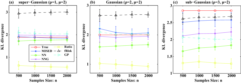
Figure 2: KL-divergence estimation for (a) super-Gaussian, (b) Gaussian and (c) sub-Gaussian data as a function of sample size $n$.

3.4 Numerical Examples

We experimentally compare the behavior of the NNDE-based KL-divergence approximator with MISED-based metric learning (MISED), that without metric learning (NN) [19], that with Gaussian-based metric learning (NNG) [6], the density-ratio-based non-parametric KL-divergence estimator (Ratio) [21], the risk-based nearest-neighbor KL-divergence estimator (fRisk) [22], and the Gaussian parametric KL-divergence estimator with maximum likelihood estimation (GP).

We generate data samples from the generalized Gaussian distribution:

$$p_{\mathrm{GG}}(x;\mu,\beta,\rho) =\frac{\beta^{1/2}}{2\Gamma(1+1/\rho)}\exp\left(-\beta^{\rho/2}|x-\mu|^{\rho}\right),$$

where $\mu\in\mathbb{R}$ denotes the mean, $\beta>0$ controls the variance, and $\rho>0$ controls the Gaussianity: $\rho<2$, $\rho=2$, and $\rho>2$ correspond to super-Gaussian, Gaussian, and sub-Gaussian distributions, respectively. For $\boldsymbol{x}=(x^{(1)},\ldots,x^{(d)})^{\top}$ with $d=5$, we set

$$p_{1}(\boldsymbol{x}) =\prod_{j=1}^{d}p_{\mathrm{GG}}(x^{(j)};0,\beta,\rho),$$

$$p_{2}(\boldsymbol{x}) =p_{\mathrm{GG}}(x^{(1)};2,\beta,\rho)\prod_{j=2}^{d}p_{\mathrm{GG}}(x^{(j)};0,\beta,\rho),$$

where the value of $\beta$ is selected so that the variance is one. We evaluate the performance of each method when sample size $n$ and Gaussianity $\rho$ are changed.

The experimental results for $\rho=1,2,3$ and $n=500,1000,1500,2000$ are presented in Figure 2. The proposed MISED outperforms the plain NN (without metric learning) for all three cases, and it outperforms NNG and GP for the super-Gaussian and sub-Gaussian cases. GP and NNG work the best for the Gaussian case as expected, but MISED also still works reasonably well. fRisk is better than MISED for the sub-Gaussian case, but it largely overestimates for the other two cases. Ratio is a completely non-parametric method, but it systematically underestimates for all three cases.

3.5 Experiments on Distributional Change Detection

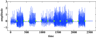
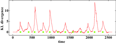
(a) Example 1

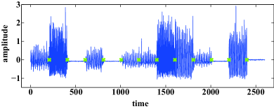
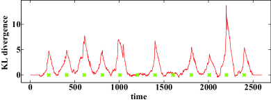
(b) Example 2

Figure 3: HASC time series data (top) and the KL-divergence estimated by MISED (bottom). Green symbols represent the true change points.

Table 1: Means and standard deviations of the area under the ROC curve (AUC) over $10$ runs. The best method and methods comparable to the best one in terms of the mean AUC by the one-tailed Welch’s t-test with significance level $5\%$ are highlighted in boldface.

GP	NNG [6]	fRisk [22]	MISED
0.747(0.050)	0.822(0.030)	0.858(0.022)	0.839(0.028)

The goal of change detection is to find abrupt changes in time-series data. We use an $m$-dimensional real vector $\boldsymbol{y}(t)$ to represent a segment of time series at time $t$, and a collection of $r$ such vectors is obtained from a sliding window:

$$\boldsymbol{Y}(t):=\{\boldsymbol{y}(t),\boldsymbol{y}(t+1),\ldots,\boldsymbol{y}(t+r-1)\}.$$

Following [18], we consider an underlying density function that generates $r$ retrospective vectors in $\boldsymbol{Y}(t)$. We measure the KL-divergence between the underlying density functions of the two sets, $\boldsymbol{Y}(t)$ and $\boldsymbol{Y}(t+r+m)$ for every $t$, and determine a point $t_{0}+r+m$ as a change point if the KL-divergence for $\boldsymbol{Y}(t_{0})$ and $\boldsymbol{Y}(t_{0}+r+m)$ is greater than a predefined threshold. In the experiment, we set $r=3$ and $m=100$.

We use the Human Activity Sensing Consortium (HASC) Challenge 2011 collection, which provides human activity information collected by a portable three-axis accelerometer. Our task is to segment different activities such as “stay”, “walk”, “jog”, and “skip”. Because the orientation of the accelerometer is not necessarily fixed, we took the $\ell_{2}$-norm of 3-dimensional accelerometer data and obtained one-dimensional data, following [18].

Figure 3 depicts examples of time-series data and their KL-divergences (which is regarded as a change score). These graphs show that the change scores tend to be large at the true change points. Next, we more systematically evaluate the performance of change detection using the AUC (area under the ROC curve) scores. The results are summarized in Table 1, showing that the proposed MISED outperforms GP and NNG, and is comparable to fRisk. In the experiments in Figure 2, fRisk gave similar values for different distributions even when the true KL-divergence is large. This was poor as a KL-divergence approximator, but this property seems to work as a “regularizer” to stabilize the change score to avoid incurring big error. Similar tendencies were also reported in the previous work [6].

3.6 Experiments on Information-Theoretic Feature Selection

Finally, KL-divergence approximation is applied to selecting relevant features for classification. The Jensen-Shannon (JS) divergence is an information-theoretic measure between labels $y\in\{1,2\}$ and features $\boldsymbol{x}\in\mathbb{R}^{d}$:

$$\mathrm{JS}(\mathcal{X};\boldsymbol{y}) =-\sum_{y=1}^{2}\int p(\boldsymbol{x},y)\log\frac{p(\boldsymbol{x})p(y)}{p(\boldsymbol{x},y)}\mathrm{d}\boldsymbol{x}$$

$$=p(y=1)\mathrm{KL}(p(\boldsymbol{x}|y=1)\|p(\boldsymbol{x}))$$

$$\phantom{=}+p(y=2)\mathrm{KL}(p(\boldsymbol{x}|y=2)\|p(\boldsymbol{x})),$$

where $p(\boldsymbol{x})=p(y=1)p(\boldsymbol{x}|y=1)+p(y=2)p(\boldsymbol{x}|y=2)$.

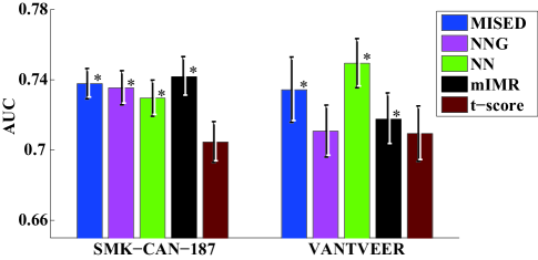
Figure 4: Gene expression classification with feature selection. The best method and methods comparable to the best one in terms of the mean AUC by the one-tailed Welch’s t-test with significance level $5\%$ are highlighted by the asterisks.

We use two gene expression datasets of breast cancer prognosis studies: “SMK-CAN-187” [23] and “VANTVEER” [24]. The SMK-CAN-187 dataset contains 90 positive (alive) and 97 negative (dead after 5 years) samples with 19993 features. We use 65 randomly selected samples per class for training and use the rest for evaluating the test classification performance. The VANTVEER dataset contains 46 positive and 51 negative samples with 24481 features. We use 35 randomly selected data per class for training and use the rest for evaluating the test classification performance.

We choose $20$ features based on the forward selection strategy and compare the AUC of classification. The results are summarized in Figure 4, showing that the proposed method works reasonably well.

4 Conclusion

We proposed a method to directly estimate density derivatives. The proposed estimator, called MISED, was shown to possess various useful properties, e.g., analytic and computationally efficient estimation of multi-dimensional high-order density derivatives is possible and all hyper-parameters can be chosen objectively by cross-validation. We further proposed a MISED-based metric learning method to improve the accuracy of nearest-neighbor KL-divergence approximation, and its practical usefulness was experimentally demonstrated on change detection and feature selection.

Estimation of density derivatives is versatile and useful in various machine learning tasks beyond KL-divergence approximation. In our future work, we will explore more applications based on the proposed MISED method.

References

- [1] K. Fukunaga and L. Hostetler. The estimation of the gradient of a density function, with applications in pattern recognition. IEEE Transactions on Information Theory, 21(1):32–40, 1975.
- [2] Y. Cheng. Mean shift, mode seeking, and clustering. IEEE Transactions on Pattern Analysis and Machine Intelligence, 17(8):790–799, 1995.
- [3] D. Comaniciu and P. Meer. Mean shift: A robust approach toward feature space analysis. IEEE Transactions on Pattern Analysis and Machine Intelligence, 24(5):603–619, 2002.
- [4] H. Sasaki, A. Hyvärinen, and M. Sugiyama. Clustering via mode seeking by direct estimation of the gradient of a log-density. In Proceedings of the European Conference on Machine Learning and Principles and Practice of Knowledge Discovery in Databases (ECML/PKDD 2014), to appear, 2014.
- [5] B.W. Silverman. Density estimation for statistics and data analysis. CRC press, 1986.
- [6] Y. K. Noh, M. Sugiyama, S. Liu, M. C. du Plessis, F. C. Park, and D. D. Lee. Bias reduction and metric learning for nearest-neighbor estimation of kullback-leibler divergence. In Proceedings of the 17th International Conference on Artificial Intelligence and Statistics (AISTATS), pages 669–677, 2014.
- [7] R.S. Singh. Applications of estimators of a density and its derivatives to certain statistical problems. Journal of the Royal Statistical Society. Series B, 39(3):357–363, 1977.
- [8] P.K. Bhattacharya. Estimation of a probability density function and its derivatives. Sankhyā: The Indian Journal of Statistics, Series A, 29(4):373–382, 1967.
- [9] E.F. Schuster. Estimation of a probability density function and its derivatives. The Annals of Mathematical Statistics, 40(4):1187–1195, 1969.
- [10] W. Hardle, J.S. Marron, and M.P. Wand. Bandwidth choice for density derivatives. Journal of the Royal Statistical Society, Series B, 52(1):223–232, 1990.
- [11] R.S. Singh. Improvement on some known nonparametric uniformly consistent estimators of derivatives of a density. The Annals of Statistics, 5(2):394–399, 1977.
- [12] R.S. Singh. On the exact asymptotic behavior of estimators of a density and its derivatives. The Annals of Statistics, 9(2):453–456, 1981.
- [13] A. Hyvärinen. Estimation of non-normalized statistical models by score matching. Journal of Machine Learning Research, 6:695–709, 2005.
- [14] J. Kim and C. Scott. kernel classification. IEEE Transactions on Pattern Analysis and Machine Intelligence, 32(10):1822–1831, 2010.
- [15] M. Sugiyama, T. Suzuki, T. Kanamori, M. C. du Plessis, S. Liu, and I. Takeuchi. Density-difference estimation. Neural Computation, 25(10):2734–2775, 2013.
- [16] T. Kanamori, T. Suzuki, and M. Sugiyama. -divergence estimation and two-sample homogeneity test under semiparametric density-ratio models. IEEE Transactions on Information Theory, 58(2):708–720, 2012.
- [17] G. Brown. A new perspective for information theoretic feature selection. Journal of Machine Learning Research - Proceedings Track, 5:49–56, 2009.
- [18] S. Liu, M. Yamada, N. Collier, and M. Sugiyama. Change-point detection in time-series data by relative density-ratio estimation. Neural Networks, 43:72–83, 2013.
- [19] Q. Wang, S. R. Kulkarni, and S. Verdu. A nearest-neighbor approach to estimating divergence between continuous random vectors. IEEE Transactions on Pattern Analysis and Machine Intelligence, 55(5):2392–2405, 2006.
- [20] T. Kanamori, S. Hido, and M. Sugiyama. A least-squares approach to direct importance estimation. The Journal of Machine Learning Research, 10:1391–1445, 2009.
- [21] X. Nguyen, M. J. Wainwright, and M. I. Jordan. Estimating divergence functionals and the likelihood ratio by convex risk minimization. IEEE Transactions on Information Theory, 56(11):5847–5861, 2010.
- [22] D. Garcia-Garcia, U. von Luxburg, and R. Santos-Rodriguez. Risk-based generalizations of -divergences. In Proceedings of 28th International Conference on Machine Learning, pages 417–424, 2011.
- [23] W. A. Freije, et al. Gene expression profiling of gliomas strongly predicts survival. Cancer Research, 15;64(18):6503–6510, 2004.
- [24] A. Spira, et al. Airway epithelial gene expression in the diagnostic evaluation of smokers with suspect lung cancer. Nature Medicine, 13(3):361–6, 2007.