Geo-Social Group Queries with Minimum Acquaintance Constraints

Abstract

The prosperity of location-based social networking has paved the way for new applications of group-based activity planning and marketing. While such applications heavily rely on geo-social group queries (GSGQs), existing studies fail to produce a cohesive group in terms of user acquaintance. In this paper, we propose a new family of GSGQs with minimum acquaintance constraints. They are more appealing to users as they guarantee a worst-case acquaintance level in the result group. For efficient processing of GSGQs on large location-based social networks, we devise two social-aware spatial index structures, namely SaR-tree and SaR*-tree. The latter improves on the former by considering both spatial and social distances when clustering objects. Based on SaR-tree and SaR*-tree, novel algorithms are developed to process various GSGQs. Extensive experiments on real datasets Gowalla and Twitter show that our proposed methods substantially outperform the baseline algorithms under various system settings.

1 Introduction

With the ever-growing popularity of smartphone devices, the past few years have witnessed a massive boom in location-based social networking services (LBSN) Zhang15 ; Hao15 ; Schlegel15 ; Khalid15 like Foursquare, Yelp, Google+, and Facebook Places. In all these applications, mobile users are allowed to share their check-in locations (e.g., restaurants, theaters) with friends. Such location information, bridging the gap between the physical world and the virtual world of social networks, presents to users new applications of group-based activity planning and marketing yang12 ; yafei15 ; yafei17 . In a typical use case, Facebook now offers users to create or participate a local group event, such as a lunch gathering or a tennis match. With location information, Facebook can proactively recommend users nearby and invite them to this event. Third-party apps can also make use of such information. For example Zimride, on Facebook suggests ridesharing among a group of users with similar commutes. These location-based social networking applications are essentially geo-social group queries with both spatial and social constraints.

While research attention has recently been drawn to geo-social group queries (e.g., liu ; yang12 ), existing works only impose some loose social constraint on the query. For example in liu , the circle-of-friend query targets at finding a set of $k$ users such that the maximal weighted spatial and social distance among the users is minimized. Since social distance is only one of the two factors, users in the result group could have very distant or diverse social relations. In an extreme case, no users in the result group are familiar with one another but they are so spatially close that the overall intra-group distance is minimum. As an improvement, the socio-spatial group query proposed in yang12 aims to find $k$ spatially close users among which the average number of unfamiliar users does not exceed a threshold $p$. While the use of threshold $p$ effectively reduces the occurrence of unfamiliar users in a result group, there is no guarantee on the minimum number of users a group member is familiar with. In the worst case, as shown in our experiments in Section 7.2, some user may be unfamiliar with all other users in the group. Moreover, both queries require tailor-made user inputs — liu imposes weights on social and spatial distances, and yang12 needs to set a unified threshold $p$ for all users in the group even though different users may have varied tolerance of unfamiliar users surrounded. Finally, these works mainly focused on in-memory processing (e.g., improving the user scanning order and filtering the candidate combinations), and cannot be adapted to external-memory indexes. Therefore, they cannot work for large-scale and real-world LBSNs.

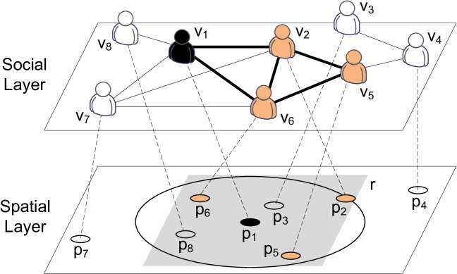
Figure 1: An example of GSGQ$<$$v_{1},3NN,2$$>$. Lines between the users represent acquaintance relations and the points on the spatial layer denote the positions of the users.

In this paper, we propose a new family of Geo-Social Group Queries with constraint on minimum acquaintance, hereafter called GSGQs for brevity. A GSGQ query takes three arguments: $(q,\Lambda,c)$, where $q$ is the query issuer, $\Lambda$ is the spatial constraint, and $c$ is the acquaintance constraint. The acquaintance constraint $c$ imposes a minimum degree on the familiarity of group members (which may include $q$), i.e., every user in the group should be familiar with at least $c$ other users. The minimum degree constraint is an important measure of group cohesiveness in social science research seidman . Known as $c$-core, it has been widely investigated in the research of graph problems balas ; cheng ; moser and accepted as an important constraint in practical applications sozio . The spatial constraint $\Lambda$ can be a range constraint, a $k$-nearest-neighbor ($k$NN) constraint or a relaxed $k$-nearest-neighbor (r$k$NN) constraint, where $k$NN (resp. r$k$NN) means the result group, among all valid groups of exactly (resp. no fewer than) $k$ users that satisfy the minimum acquaintance constraint, has the minimum spatial distance to the query issuer.

Fig. 1 illustrates an example of GSGQ, where the social network is split into a social layer and a spatial layer for clarify of presentation. Suppose user $v_{1}$ wants to arrange a friend gathering of some friends nearby. To have a friendly atmosphere in the gathering, she hopes anyone in the group should be familiar with at least two other users. Thus, she issues a GSGQ $=(q,\Lambda,c)$ with $q$ set as $v_{1}$, $\Lambda$ being $3$NN, and $c=2$. With the objective of minimizing the spatial distance between $q$ and the farthest user in the group, the result group she will obtain is $W=\{v_{2},v_{5},v_{6}\}$. Alternatively, to find an acquainted group of friends within a fixed range, she may issue a GSGQ $=(q,\Lambda,c)$ with $q$ set as $v_{1}$, $\Lambda$ being $r$ (shaded area in Fig. 1), and $c=2$. In this example, she will also obtain $W=\{v_{2},v_{5},v_{6}\}$.

We argue that, compared to the geo-social group queries studied in prior work liu ; yang12 , our GSGQs, with the adoption of a minimum acquaintance constraint, are more appealing to produce a cohesive group that guarantees the worst-case acquaintance level. Nonetheless, these GSGQs are much more complex to process than conventional spatial queries. Particularly, when the spatial constraint is strict $k$NN, we prove that GSGQs are NP-hard. Due to the additional social constraint, traditional spatial query processing techniques finkel ; guttm ; beckmann ; papad cannot be directly applied to GSGQs. Moreover, these queries are intrinsically harder than other variants of spatial queries, such as spatial-keyword queries feli ; zhang ; wu and collective spatial keyword queries cao , which only introduce independent attributes (e.g., text descriptions) of the objects but not binary relations among them.

On the other hand, most previous works on group queries in social networks use sequential scan in query processing. That is, they enumerate every possible combination of a user group and optimize the processing through some pruning heuristics. Although yang12 proposed an SR-tree to cluster the users of each leaf node, this index achieves more significant reduction on computation than on disk accesses since it separates spatial and social constraints in the clustering process. Thus, when geo-social queries such as GSGQs are processed, still many disk pages are accessed to fetch the users that satisfy both spatial and social constraints. Moreover, its filtering techniques only work for average-degree social constraints, and are not suitable for GSGQs with minimum-degree social constraints. In this paper, we propose two novel social-aware spatial indexing structures, namely, SaR-tree and SaR*-tree, for efficient processing of general GSGQ queries on external storage. The main idea is to project the social relations of an LBSN on the spatial layer and then index both social and spatial relations in a uniform tree structure to facilitate GSGQ processing. Furthermore, we optimize the in-memory processing of GSGQs with a strict $k$NN constraint by devising powerful pruning strategies. To sum up, the main contributions of this paper are as follows:

• We propose a new family of geo-social group queries with minimum acquaintance constraint (GSGQs), which guarantees the worst-case acquaintance level. We prove that the GSGQs with a strict $k$NN spatial constraint are NP-hard.

• We design new social-aware index structures, namely SaR-tree and SaR*-tree, for GSGQs. To optimize the I/O access and processing cost, a novel clustering technique that considers both spatial and social factors is proposed in the SaR*-tree. The update procedures of both indexes are also presented.

• Based on the SaR-tree and SaR*-tree, efficient algorithms are developed to process various GSGQs. Moreover, in-memory optimizations are proposed for GSGQs with a strict $k$NN constraint.

• We conduct extensive experiments to demonstrate the performance of our proposed indexes and algorithms.

The rest of this paper is organized as follows. Section 2 reviews the related works. Section 3 introduces some core concepts in the social constraint and formalizes the problems of GSGQs. Section 4 presents the designs of basic SaR-tree and optimized SaR*-tree. Section 5 details the processing methods for various GSGQs based on SaR-trees. Section 6 describes the update algorithms of SaR-trees. Section 7 evaluates the performance of our proposals. Finally, Section 8 concludes the paper and discusses future directions.

2 Related Works

2.1 Spatial Query Processing

Many spatial databases use R-tree or its extensions guttm ; beckmann as an access method to disk storage for spatial queries (e.g., range, $k$NN, and spatial join queries). Fig. 2 shows nine objects in a two-dimensional space and how they are aggregated into Minimum Bounding Rectangles (MBRs) recursively to build up the corresponding R-tree. An R-tree node is composed of a number of entries, each covering a set of objects and using an MBR to bound them. A query is processed by traversing the R-tree from the root node all the way down to leaf nodes for qualified objects. During this process, a priority queue $H$ can be used to maintain the entries to be explored. A generic query evaluation procedure for a query $Q$ can be summarized as follows: (1) push the entries of the root node into $H$; (2) pop up the top entry $e$ from $H$; (3) if $e$ is a leaf entry, check if the corresponding object is a result object; otherwise push all qualified child entries of $e$ into $H$; (4) repeat (2) and (3) until $H$ is empty or a termination condition of $Q$ is satisfied. The construction of R-trees can be either incremental guttm ; beckmann or bulk-loaded.

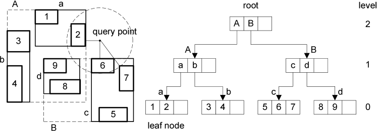
Figure 2: An example of R-tree.

Some variants of spatial queries have been studied with the consideration of certain grouping semantics. The group nearest-neighbor query papad extends the concept of the nearest neighbor query by considering a group of query points. It targets at finding a set of data points with the smallest sum of distances to all the query points. Based on R-tree, papad proposes various pruning heuristics to efficiently process group nearest-neighbor queries. The spatial-keyword query is another well-known extension of spatial queries that exploits both locations and textual descriptions of the objects. Most solutions for this query, e.g., BR*-tree zhang , $IR^{2}$-tree feli , and IR-tree wu , rely on combining the inverted index, which was designed for keyword search, with a conventional R-tree. The collective spatial keyword query cao further considers the problem of retrieving a group of spatial web objects such that the group’s keywords cover the query’s keywords and the objects, with the shortest inter-object distances, are nearest to the query location. Based on IR-tree, cao proposes dynamic programming algorithms for exact query processing and greedy algorithms for approximate query processing. It is noteworthy that, while these works deal with some grouping semantics, they do not consider acquaintance relations in social networks.

2.2 Social Network Analysis and Query Processing

There have been a lot of works on community discovery in social networks. There is a comprehensive survey on community finding in graphs fortunato . A typical approach is to optimize the modularity measure girvan . Since communities are usually cohesive subgraphs formed by the users with the acquaintance relationship, some graph structures such as clique harary , $k$-core seidman , and $k$-plex balas ; mcclosky ; moser have been well studied under this topic. However, most of these works only provide theoretical solutions with asymptotic complexity, with a few exceptions such as the external-memory top-down algorithm for core decomposition cheng .

As for query processing in social networks, faloutsos addresses the problem of finding a subgraph that connects a set of query nodes in a graph. sozio studies a query-dependent variant of the community discovery problem, which finds a dense subgraph that contains the query nodes. Based on a measure of graph density, an optimal greedy algorithm is proposed. The authors of sozio also prove that finding communities of size no larger than a specified upper bound is NP-hard. Besides, yang proposes a social-temporal group query with acquaintance constraint in social networks. The aim is to find the activity time and attendees with the minimum total social distance to the initiator. As this problem is NP-hard, heuristic-based algorithms have been proposed to reduce the run-time complexity. However, all these works do not consider the spatial dimension of the users and thus cannot be applied to location-based social networks.

2.3 Geo-Social Query Processing

Efficient processing of queries that consider both spatial and social relations is essential for LBSNs. doyt directly combines spatial and social networks and proposes graph-based query processing techniques. liu proposes a circle-of-friend query to find minimal-diameter social groups. By transforming the relations in social networks into social distances among users, an integrated distance combining both spatial and social distances is proposed. yang12 considers a special socio-spatial group query with the requirement of minimizing the total spatial distance. Accordingly, in-memory pruning and searching schemes are proposed in yang12 . All these works only impose a loose social constraint in the query. As for the processing techniques, the methods of these works enumerate all possible combinations guided by some searching and pruning schemes. Although a tree structure named SR-tree is introduced in yang12 , it is mainly used to reduce the enumeration of states during the in-memory processing. With that said, external-memory indexes tailored for geo-social query processing in large-scale LBSNs are still lacking. More recently, Armenatzoglou proposes a general framework for geo-social query processing, which separates the social, geographical and query processing modules and thus enables flexible data management. Since its pruning power comes separately from the social and spatial index, it cannot further optimize the processing of GSGQ with access methods that integrate both spatial and social information. yafei15 studies a geo-social query that retrieves a group of socially connected users whose familiar regions collectively cover a set of query points. Zhang13 proposes a geo-social location recommendation system based on personalized social and geographical influence modeling. Similarly, Shi14 proposes to cluster and categorize locations based on social and spatial density obtained from geo-social networks.

3 Preliminaries and Problem Statement

Aiming to find a cohesive group of acquaintances, GSGQs use $c$-core seidman as the basis of social constraint to restrict the result group. In this section, we first introduce the definition and the properties of $c$-core, based on which the GSGQ problems are then formalized.

3.1 $C$-Core

$c$-core is a degree-based relaxation of clique seidman . Consider an undirected graph $G=(V,E)$, where $V$ is the set of vertices and $E$ is the set of edges. Given a vertex $v\in V$, we define the set of neighbors of $v$ as $N_{G}(v)=\{u\in V~{}|~{}uv\in E\}$ and the degree of $v$ as $deg_{G}(v)=|N_{G}(v)|$. Accordingly, the maximum and minimum degrees of $G$ are represented as $\Delta(G)=max_{v\in V}{deg_{G}(v)}$ and $\delta(G)=min_{v\in V}{deg_{G}(v)}$, respectively. Let $G[W]$ denote a subgraph induced by $W\subseteq V$. The following is a generalized definition of a $c$-core seidman .

Definition 1

($c$-core) A subgraph $G[W]$ is a c-core (or a core of order c) if $\delta(G[W])\geq c$.

The $c$-core defined in Definition 1 is not required to be maximum and fits for GSGQs in various applications. In the sequel, the term $c$-core refers to both the set $W$ and the subgraph $G[W]$. The core number of a vertex $v$, denoted by $c_{v}$, is the highest order of a core that contains this vertex.

A greedy algorithm can be used for core decomposition, i.e., finding the core numbers for all vertices in $G$. The basic idea is to iteratively remove the vertex with the minimum degree in the remaining subgraph, together with all the edges adjacent to it, and determine the core number of that vertex accordingly. The most costly step of this algorithm is sorting the vertices according to their degrees at each iteration. As shown in batag , a bin-sort can be used with $O(|V|+|E|)$ time complexity. Thus, for a given $c$, we can find the maximum $c$-core of $G$ in $O(|V|+|E|)$ time.

3.2 Problem Statement

Consider an LBSN $G=(V,E)$, where the set of vertices $V$ denotes the users and the set of edges $E$ denotes the acquaintance relations among the users in $V$. For any two users $v,u\in V$, there exists an edge $vu\in E$ if and only if $v$ is acquainted with $u$. Moreover, for any user $v\in V$, its location $p_{v}$ is also stored in $G$. Given two users $v$ and $u$, let $d(v,u)$ denote the spatial distance between $v$ and $u$, and the (largest) distance from $v$ to a set of users $W$ is defined by $d_{max}(v,W)=max_{u\in W}{d(v,u)}$.

As formally defined below, a GSGQ finds a group of users that satisfies the given spatial and social constraints. Without loss of generality, we assume that the query issuer $q\in V$.

Definition 2

(Geo-Social Group Query with Minimum Acquaintance Constraint (GSGQ)) Given an LBSN $G=(V,E)$, a GSGQ is represented as $Q_{gs}=(v,\Lambda,c)$, where $v\in V$ is the query issuer, $\Lambda$ is a type of spatial query denoting the spatial constraint, and $c$ is the minimum degree of result group, denoting the social acquaintance constraint as in liu ; yang12 . GSGQ finds a maximal user result set $W$ which satisfies $\Lambda$ and the condition that the induced subgraph $G[W\cup\{v\}]$ is a $c$-core, or formally, $\delta(G[W\cup\{v\}])~{}\geq~{}c$.

As for the spatial constraint, this paper mainly focuses on three query types: range (i.e., window) query, relaxed k-nearest-neighbor (r$k$NN) query, and strict k-nearest-neighbor ($k$NN) query. Accordingly, they correspond to three types of GSGQs:

• GSGQ with range constraint, denoted as $GSGQ_{range}$. A $GSGQ_{range}$ is represented as $Q_{gs}=(v,range,c)$, where $p_{v}\in range$. It targets at finding the largest $c$-core $W\cup\{v\}$ located inside $range$, a rectangular spatial window. For example, “find me the largest user group satisfying $c$-core in 5th Avenue, Manhattan, NYC.”

• GSGQ with relaxed $k$NN constraint, denoted as $GSGQ$ _rkNN. A $GSGQ_{rkNN}$ is represented as $Q_{gs}=(v,rkNN,$ $c)$. It targets at finding a maximal $c$-core $W\cup\{v\}$ of size no less than $k+1$ with the minimum $d_{max}(v,W)$. Here “relaxed” means the size of the result is not strictly $k+1$, and as a general requirement in GSGQ the size should be the largest possible. For example, “find me the closest (maximal) group of at least 9 users satisfying $c$-core to be eligible for a bulk discount.”

• GSGQ with strict $k$NN constraint, denoted as $GSGQ_{kNN}$. A $GSGQ_{kNN}$ is represented as $Q_{gs}=(v,$ $kNN,c)$. It is a strict form of $GSGQ_{rkNN}$, which requires that the $c$-core $W\cup\{v\}$ has an exact size of $k+1$. For example, “find me the closest group of 3 users satisfying $c$-core to play tennis doubles with me.”

For these GSGQs, we prove the following theorems on their complexities.

Theorem 3.1

$GSGQ_{range}$ and $GSGQ_{rkNN}$ can be solved in polynomial time.

Proof

As we will show in the next subsection, processing a $GSGQ_{range}$ can be completed by running core-decomposition once, while processing a $GSGQ_{rkNN}$ can be completed by running core-decomposition at most $|V|$ times. Since the time complexity of core-decomposition is $O(|V|+|E|)$, both of the queries can be solved in polynomial time.

Theorem 3.2

$GSGQ_{kNN}$ is NP-hard.

Proof

It has been proved in balas that, given a graph $G$ and positive integers $\bar{c}$ and $k$, determining whether there exists a $\bar{c}$-plex of size $k+1$, i.e., a set $W$ such that $\delta(G[W])\geq|W|-\bar{c}$ and $|W|=k+1$, is NP-complete. Since a $c$-core of size $k+1$ is equivalent to a $(k+1-c)$-plex, we can find a $(k+1-c)$-plex of size $k+1$ by iteratively applying $GSGQ_{kNN}$ for each user $v$ in $G$. If a $c$-core of size $k+1$ is found for a user $v$, then a $(k+1-c)$-plex of size $k+1$ exists; otherwise such a $(k+1-c)$-plex does not exist. In this way, the $\bar{c}$-plex problem can be polynomially reduced to $GSGQ_{kNN}$. This proves that $GSGQ_{kNN}$ is NP-hard.

3.3 R-tree based Query Processing

We consider the GSGQ problems for large-scale LBSNs where the users’ location and social information are stored separately on external disk storage as described in Armenatzoglou . A baseline approach of processing GSGQs on an R-tree index of user locations is as follows. For a $GSGQ_{range}$ $Q_{gs}=(v,range,c)$, we first find all users located inside $range$ via R-tree, then compute the $c$-core $W^{\prime}$ of the subgraph formed by these users. If $v$ exists in $W^{\prime}$, then $W=W^{\prime}-\{v\}$ is the final result; otherwise, there is no result for $Q_{gs}$. Since the user filtering step can be done in $O(|V|)$ time and the core decomposition step can be done in $O(|V|+|E|)$ time, the complexity of this method is $O(|V|+|E|)$.

For a $GSGQ_{rkNN}$ $Q_{gs}=(v,rkNN,c)$, according to its definition, we access the users in ascending order of their spatial distances to $v$. As such, we use a similar procedure to kNN search on R-tree. Specifically, we employ a priority queue $H$ whose priority score is spatial distance to $v$, and a candidate result set $\widetilde{W}$. At the beginning, $\widetilde{W}$ is initialized as $\{v\}$ and all the root entries of the R-tree are put into $H$. Each time the top entry $e$ of $H$ is popped up and processed. If $e$ is a non-leaf entry, its child entries are accessed and put into $H$; otherwise, $e$ is a leaf entry, i.e., a user, so $e$ is added into $\widetilde{W}$. When the size of $\widetilde{W}$ exceeds $k$, we compute the $c$-core $W^{\prime}$ of the subgraph formed by the users in $\widetilde{W}$. If $|W^{\prime}|\geq k+1$ and $v\in W^{\prime}$, $W=W^{\prime}-\{v\}$ is the result; otherwise, the above procedure is continued until the result is found. Since each round of $c$-core detection can be done in $O(|V|+|E|)$ time, the complexity of this method is $O(|V|(|V|+|E|))$.

For a $GSGQ_{kNN}$ $Q_{gs}=(v,kNN,c)$, the processing is similar to $GSGQ_{rkNN}$. The major difference is how to find the result from $\widetilde{W}$. Since the query returns exact $k$ users, all possible user sets of size $k+1$ and containing $v$ are checked to see if it is a $c$-core. If such a user set $W^{\prime}$ exists, then $W=W^{\prime}-\{v\}$ is the result. There are $C^{|V-1|}_{k}$ possible user sets to be checked, where $C^{|V-1|}_{k}$ denotes the number of $k$-combinations from the user set $V-\{v\}$. Thus, the complexity of this method is $O(C^{|V-1|}_{k}(|V|+|E|))$,

Obviously, these approaches are inefficient for GSGQs with a large $c$ value, because a large $c$ means tighter social constraints and thus result users from farther away. According to a recent study Shin16 , the maximum $c$ of a graph where the $c$-core exists obeys a 3-to-1 power law with respect to the count of triangles in the graph. This implies that the number of users to search and check in these approaches increases exponentially as $c$ increases. On the other hand, intuitively a large $c$ means higher chances to prune the irrelevant users before finding the result users. As will be proved and shown in the rest of this paper, the efficiency can be significantly improved by filtering the irrelevant users and optimizing the processing order.

4 Social-aware R-trees

Since a GSGQ involves both spatial and social constraints, to expedite its processing, both spatial locations and social relations of the users should be indexed simultaneously. Unfortunately, R-tree only indexes spatial locations of the users and is thus inefficient. In this section, we design novel Social-aware R-trees (SaR-trees) to form the basis of our query processing solutions. In what follows, we first introduce the concept of Core Bounding Rectangle (CBR) and then present the details of SaR-tree, followed by a variant SaR*-tree.

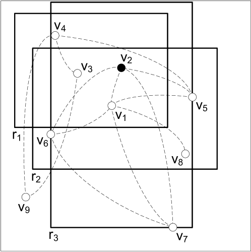
Figure 3: An example of CBR. The LBSN is shown on the spatial layer. The points represent the users as well as their positions, while the dashed lines denote the acquaintance relations among users.

4.1 Core Bounding Rectangle (CBR)

The social constraint of a GSGQ requires the result group to be a $c$-core. Unfortunately, pure social measures such as core number and centrality cannot adequately facilitate GSGQ processing which also features a spatial constraint. To devise effective spatial-dependant social measures to filter users in query processing, in this paper, we develop the concept of Core Bounding Rectangle (CBR) by projecting the minimum degree constraint on the spatial layer. Simply put, the CBR of a user $v$ is a rectangle containing $v$, inside which any user group with $v$ does not satisfy the minimum degree constraint. In other words, it is a localized social measure to a user. As a GSGQ mainly requests the nearby users, the locality of CBR becomes very valuable for processing GSGQs. The formal description of a CBR of user $v$ for a minimum degree constraint $c$, denoted by $CBR_{v,c}$, is given in Definition 3.

Definition 3

(Core Bounding Rectangle (CBR)) Consider a user $v\in G$. Given a minimum degree constraint $c$, $CBR_{v,c}$ is a rectangle which contains $v$ and inside which any user group with $v$ (excluding the users on the bounding edges) cannot be a $c$-core. Formally, $CBR_{v,c}$ satisfies $p_{v}\in CBR_{v,c}$ and $\forall W=\{v\}\cup\{u|u\in V,p_{u}\in CBR_{v,c}\}$ $\delta(G[W])<c$.

An example is shown in Fig. 3. According to the acquaintance relations of user $v_{2}$, rectangular area $r_{1}$ is a $CBR$ ${}_{v_{2},2}$, because any user group inside $r_{1}$ that contains $v_{2}$ cannot be a $2$-core. On the contrary, $r_{2}$ is not a $CBR_{v_{2},2}$, because some user groups inside $r_{2}$ that contain $v_{2}$, e.g., $\{v_{2},v_{1},$ $v_{6}\}$, are $2$-cores. Note that $CBR_{v,c}$ is not unique for a given $v$ and $c$. For example, $r_{3}$ is another $CBR_{v_{2},2}$ for user $v_{2}$. From Definition 3, we can quickly exclude a user $v$ from the result group by checking $CBR_{v,c}$ during query processing. For example, if the query range of a $GSGQ_{range}$ is covered by $CBR_{v,c}$, then $v$ can be safely pruned from the result. This property makes CBR a powerful pruning mechanism.

Computing CBR of a User. In an LBSN $G$, given a user $v$ and minimum degree constraint $c$, a simple method to compute $CBR_{v,c}$ is to search neighboring users in ascending order of distance until there is a user $u$ such that the core number of $v$ in the subgraph formed by the users inside $\odot_{v,u}$ (i.e., the circle centered at $v$ with radius $d(v,u)$) is no less than $c$, i.e., all user groups located within $\odot_{v,u}$ are not qualified as a $c$-core. $CBR_{v,c}$ can then be easily derived from $\odot_{v,u}$ as follows. We first compute the bounding box of the circle and move out one bounding edge to go through $u$. Then we check the nodes inside the rectangle but outside the circle. For each of them, we move out one bounding edge to go through $u$ so that the node becomes outside of the new rectangle. An example is shown in Fig. 4(a), where a $CBR_{v_{2},2}$ is constructed based on users $v_{5}$, $v_{6}$, and $v_{8}$. This generated CBR satisfies Definition 3 since the users inside it (i.e., $v_{1},v_{2},v_{3}$) cannot form 2-core groups. However, it is not a maximal one, thus limiting its pruning power in GSGQ processing. We improve this initial $CBR_{v,c}$ by recursively expanding it from each bounding edge until no edge can be further moved outward (see Fig. 4(b)). Depending on different initial CBRs and different expanding orders, there could be a number of maximal CBRs.

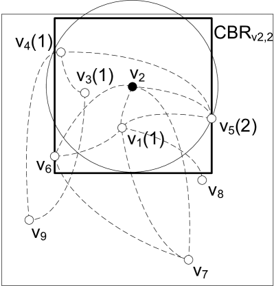
(a) Initialization

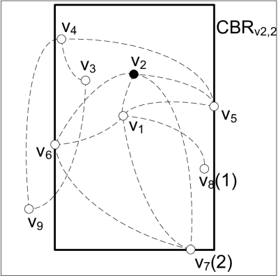
(b) Expansion

Figure 4: An exemplary procedure of computing $CBR_{v_{2},2}$ in an LBSN. The number after a user $v_{i}$ denotes the core number of $v_{2}$ in the subgraph determined by $v_{i}$. For a), the subgraph is formed by the users inside $\odot_{v_{2},v_{i}}$; for b), the subgraph is formed by the users inside $CBR_{v_{2},2}$ when moving its bottom edge outward to go through $v_{i}$.

Algorithm 1 details the procedure of computing $CBR_{v,c}$. In Line 1, we first sort the users of $V$ in ascending order of their distances to $v$. In Lines 2-5, we find the nearest user $u$ such that $c_{v}\geq c$ in the subgraph formed by the users in $V$ with equal or shorter distances to $v$. In Line 6, we initialize $CBR_{v,c}$ based on $u$ such that $CBR_{v,c}$ does not contain any user outside $\odot_{v,u}$. An exemplary way is to compute the bounding box of $\odot_{v,u}$ first and move one bounding edge to go through $u$. Then, check the users which are located inside the rectangle but outside $\odot_{v,u}$. For each of them, move one bounding edge of the rectangle to go through it so that the user is not located inside the new rectangle. In this procedure, a greedy scheme is adopted to always select the bounding edge which maximizes the area of the rectangle. In Lines 7-10, we expand $CBR_{v,c}$ by moving each bounding edge $l$ of $CBR_{v,c}$ outward, if $c_{v}<c$ in the subgraph formed by the users inside $CBR_{v,c}$ and on $l$. Obviously, the rectangle generated by Algorithm 1 is a maximal $CBR_{v,c}$, i.e., it is a $CBR_{v,c}$ and cannot be fully covered by any other $CBR_{v,c}$. This property guarantees its pruning power for GSGQ processing, and such maximal $CBR$s will be stored in the social-aware R-trees. Fig. 4 provides an exemplary procedure for computing $CBR_{v_{2},2}$ when applying Algorithm 1 on an LBSN.

Algorithm 1 Computing CBR of a User

0:  LBSN $G=(V,E)$, user $v$, constraint $c$

0:  $CBR_{v,c}$CompCBR($G$, $v$, $c$)

1:  Sort users of $V$ in ascending order of distances to $v$;

2:  for each user $u$ in $V$ do

3:    Compute $c_{v}$ in the subgraph formed by the users before (and including) $u$;

4:    if $c_{v}\geq c$ then

5:       Break;

6:    end if

7:  end for

8:  Build an initial $CBR_{v,c}$ which goes through $u$ and does not contain any user outside $\odot_{v,u}$; //$u$ is the user that breaks the above loop

9:  Sort users of $V$ in horizontal and vertical order, respectively.

10:  while existing a bounding edge $l$ of $CBR_{v,c}$ s.t. $c_{v}<c$ in the subgraph formed by the users inside $CBR_{v,c}$ and on $l$ do

11:    Move $l$ outward to the next (or previous) user in horizontal (or vertical) order until $c_{v}\geq c$ in the subgraph formed by the users inside $CBR_{v,c}$ and on $l$;

12:  end while

13:  return $CBR_{v,c}$;

To save the computing and storage cost, we only maintain a limited number of CBRs for user $v$ — $CBR_{v,2^{0}}$, $CBR_{v,2^{1}}$, $\cdots$, $CBR_{v,2^{\lfloor\log_{2}{c_{v}}\rfloor}}$ — where $c_{v}$ is the core number of $v$ in $G$. We choose CBRs with respect to exponential minimum degree constraints because for a larger $c$, as shown in Section 7, much fewer $c$-cores exist and keeping sparse CBRs is sufficient to support effective pruning.

Complexity Analysis. Let $n=|V|$ and $m=|E|$. In Algorithm 1, the sorting step, i.e., Line 1, requires $O(nlogn)$ time complexity. Since the core number of a user in graph $G$ can be computed in $O(n+m)$ time, initializing $CBR_{v,c}$ in Lines 2-6 requires $O((n+m)n)$ time complexity. Further sorting step in Line 7 requires $O(nlogn)$ time complexity. During CBR expansion in Lines 8-9, the movement of a bounding edge requires $O((n+m)n)$ time complexity. In total, the time complexity of Algorithm 1 is $O((n+m)n)$. By applying a binary search to find a proper $u$ in CBR initialization and a proper user to go through in CBR expansion, the time complexity can be reduced to $O((n+m)logn)$. Usually, $m>n$ in an LBSN, so the time complexity of Algorithm 1 is $O(mlogn)$.

4.2 SaR-tree

We now present the basic SaR-tree. It is a variant of R-tree in which each entry further maintains some aggregate social-relation information for the users covered by this entry. Fig. 5 exemplifies an SaR-tree. Different from a conventional R-tree, each entry of an SaR-tree refers to two pieces of information, i.e., a set of CBRs (detailed below) and an MBR, to describe the group of users it covers. An example of the former, $CBRs_{b}$ is shown in the figure. It comprises the core number $c_{b}$ and two CBRs $\{CBR_{b,1},CBR_{b,2}\}$ for entry $b$. The core number of an entry is the maximum core number of the users it covers, which bounds the number of CBRs of this entry. Considering that only one CBR of an entry is related to a GSGQ, we optimize the storage by decoupling CBRs from MBR, as shown in Fig. 5. Then, we can directly access the CBR page with the specified $c$, without losing any pruning power of R-tree. Perceptually, a CBR in the SaR-tree bounds a group of users from the social perspective while an MBR bounds the users from the spatial perspective. As such, SaR-tree gains the power for both social-based and spatial-based pruning during GSGQ processing, as will be explained in the next section.

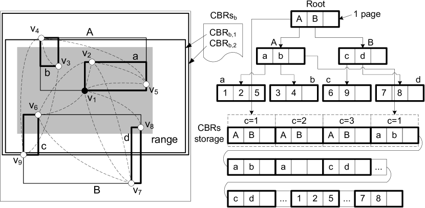
Figure 5: SaR-tree. $CBRs_{e}$ denotes the set of CBRs for an entry $e$.

CBR of an Entry. To define the CBRs for each SaR-tree entry, we extend the concept of CBR defined for each individual user (in the previous subsection). Let $MBR_{e}$ and $V_{e}$ denote the MBR and the set of users covered by an entry $e$, respectively. A CBR of $e$ is a rectangle which intersects $MBR_{e}$ and inside which any user group containing any user from $V_{e}$ cannot satisfy the minimum degree constraint. The formal definition of a CBR of entry $e$ with respect to a minimum degree constraint $c$, denoted by $CBR_{e,c}$, is given as follows:

Definition 4

(CBR of an Entry) Consider an entry $e$ with MBR $MBR_{e}$ and user set $V_{e}$. Given a minimum degree constraint $c$, $CBR_{e,c}$ is a rectangle which intersects $MBR_{e}$ and inside which any user group containing any user from $V_{e}$ (not including the users on the bounding edges) cannot be a $c$-core.

Note that $CBR_{e,c}$ is required to intersect $MBR_{e}$ to guarantee its locality. Fig. 5 shows two examples of CBRs for an entry $b$, where $V_{b}=\{v_{3},v_{4}\}$. We can see that any user group inside $CBR_{b,2}$ and containing $v_{3}$ or $v_{4}$ (not including $v_{9}$ on the bounding edges) cannot be a $2$-core. Thus, during GSGQ processing, we may safely prune entry $e$, for example, if the query range of a $GSGQ_{range}$ (with a minimum degree constraint of 2) is fully covered by $CBR_{b,2}$. Since $CBR_{e,c}$ is determined by the set of users in $V_{e}$, we use $CBR_{V_{e},c}$ and $CBR_{e,c}$ interchangeably.

To efficiently generate the CBRs of the entries in SaR-tree, we adopt a bottom-up approach in our implementation. Obviously, the CBR of a leaf entry $e$ is just the CBR of the user it covers. For a non-leaf entry $e$, let $e_{1},e_{2},\cdots,e_{m}$ be the child entries of $e$. Then, the CBR of $e$ can be computed by recursively applying the following function on $CBR_{e_{1}},$ $\ldots,CBR_{e_{m}}$:

$$CBR_{\{e_{1},\ldots,e_{i+1}\},c}=\left\{\begin{array}[]{ll}CBR_{\{e_{1},\ldots,e_{i}\},c},\text{if }{}{}{}{}{}{}{}\\ ~{}~{}~{}~{}~{}\mbox{$MBR_{e_{i+1}}\cap CBR_{\{e_{1},\ldots,e_{i}\},c}=\phi$}\\ CBR_{\{e_{1},\ldots,e_{i}\},c}\cap CBR_{e_{i+1},c},\text{ }{}{}{}{}{}{}\\ ~{}~{}~{}~{}~{}\mbox{otherwise}\\ \end{array}\right.$$

Finally, $CBR_{e,c}=CBR_{\{e_{1},\ldots,e_{m}\},c}$. It is easy to verify that the CBRs of the entries generated by the above approach satisfy Definition 4.

For an entry $e$, similar to a user, we only store the CBRs of $e$ with respect to minimum degree constraints $2^{0},2^{1},\cdots,$ $2^{\lfloor\log_{2}{c_{e}}\rfloor}$, where $c_{e}=max_{v\in V_{e}}{c_{v}}$ is the core number of $e$. Let $c_{G}$ denote the maximum core number of the users in $G$ and $s$ denote the minimum fanout of an SaR-tree. The total number of CBRs in an SaR-tree can be estimated as,

$$n_{CBR} \leq\sum_{v\in V}{(\lfloor\log_{2}{c_{v}}\rfloor+1)}+\frac{2n(\lfloor\log_{2}{c_{G}}\rfloor+1)}{s}$$

$$\leq n(\lfloor\log_{2}{\frac{\sum_{v\in V}{c_{v}}}{n}}\rfloor+\frac{2(\lfloor\log_{2}{c_{G}}\rfloor+1)}{s}+1).$$

Since $c_{G}$ and $\frac{\sum_{v\in V}{c_{v}}}{n}$ are quite small in a typical LBSN (e.g., they are 43 and 4.5 for the Gowalla dataset used in our experiments), the storage cost of CBRs is comparable to $G$ (e.g., around $2.3n$ in our experiments).

Based on the concept of CBRs, SaR-tree can be directly built on top of R-tree. That is, we first construct a standard R-tree based on the locations of the users and then embed the CBRs into each entry. In this way, SaR-tree indexes both spatial locations and social relations of the users. Note that the users in SaR-tree are organized merely based on their locations — they are spatially close, but may not be well clustered in terms of their social relations. This unfortunately weakens the pruning power of SaR-tree in processing GSGQs. To overcome this weakness, we propose a variant in the next subsection.

4.3 SaR*-tree

Inspired by R*-tree, the R-tree variant that optimizes the grouping of spatial object to minimize the disk I/O cost, we propose SaR*-tree as an variant of SaR-tree. It has the same node structure but uses a different closeness metric to group users into nodes. Specifically, instead of using only the spatial area of MBR for closeness, SaR*-tree defines a new closeness metric $I(V)$ for a group of users $V$ that integrates both CBRs and MBRs to measure the combined social and spatial closenesses:

$$I(V)=||MBR_{V}||\cdot\sum_{c}(||\cup_{v\in V}{CBR_{v,c}}-CBR_{V,c}||)$$ (1)

where $||\cdot||$ is the area of an MBR or CBR, and $\cup_{v\in V}{CBR_{v,c}}-CBR_{V,c}$ quantifies the similarity of CBRs of the users in $V$. Obviously, a small $I(V)$ indicates that the users of $V$ have both close locations and similar CBRs. This new closeness metric will be used in the R-tree construction.

Similar to SaR-tree, SaR*-tree is also constructed by iteratively inserting users. During this construction, CBRs and MBRs are generated at the same time and used for further user insertion. Moreover, if a node $N$ of an SaR*-tree overflows, it will be split. The details about these two main operations in SaR*-tree construction, i.e., user insertion and node split, are described below.

• User insertion. When a user $v$ is inserted into an SaR*-tree, for a node $N$ with entries $e_{1},e_{2},\cdots,e_{m}$, we will select the entry $e_{i}$ with the minimal $I(V_{e_{i}}\cup\{v\})$ to insert $v$.

• Node split. When a node $N$ of an SaR*-tree overflows, we split $N$ into two sets of entries $N_{1}$ and $N_{2}$ with the minimal $I($ $\cup_{e_{i}\in N_{1}}V_{e_{i}})+I(\cup_{e_{j}\in N_{2}}V_{e_{j}})$. Then, the parent node of $n$ use two entries to point to $n_{1}$ and $n_{2}$, respectively. This splitting may propagate upwards until the root.

5 GSGQ Processing

In this section, we present the detailed processing algorithms based on SaR-trees for various GSGQs. As mentioned in Section 3, we mainly focus on three types of GSGQs, namely, $GSGQ_{range}$, $GSGQ_{rkNN}$, and $GSGQ_{kNN}$. We will show that the CBRs of SaR-trees can be used in different ways for processing these queries.

5.1 GSGQ with Range Constraint

When processing a $GSGQ_{range}$ $Q_{gs}=(v,range,c)$, each entry of the SaR-tree or SaR*-tree that may cover result users will be visited and possibly further explored. Compared to traditional R-trees, which only provide spatial information via MBRs, an SaR-tree or SaR*-tree provides much greater pruning power due to the social information in CBRs. Consider an exemplary GSGQ $Q_{gs}=(v_{1},range,2)$ in Fig. 5, where the shaded area is the query range. When entry $b$ (which covers users $v_{3}$ and $v_{4}$) is visited, $b$ needs further exploration if we only consider $MBR_{b}$ like in regular R-tree. However, with $CBR_{b,2}$, we can easily decide that any user group inside the query range and containing any user in $V_{b}$ (i.e., $v_{3}$ or $v_{4}$), cannot be a $2$-core, because the query range is covered by $CBR_{b,2}$. Since $V_{b}$ does not contain any result user, we can simply prune entry $b$ from further processing, as formally proved in Theorem 5.1. Considering SaR-trees only maintain the CBRs with respect to exponential minimum degree constraints, given a minimum degree $c$, we use $CBR_{v,2^{\lfloor\log_{2}{c}\rfloor}}$ to represent $CBR_{v,c}$ in $GSGQ_{range}$ processing. Similar ideas are also applied in $GSGQ_{rkNN}$ and $GSGQ_{kNN}$ processing.

Theorem 5.1

For a $GSGQ_{range}$ $Q_{gs}=(v,range,c)$ where $p_{v}\in range$, any user in $V_{e}$ of entry $e$ does not belong to the result group if $range\subset CBR_{e,c}$ and $range$ does not contain any bounding edge of $CBR_{e,c}$.

Proof

We prove it by contradiction. If the theorem is not true, i.e., a user $u\in V_{e}$ belongs to the result group $W$. Since the users of $W\cup\{v\}$ are located inside $range$ and $range\subset CBR_{e,c}$ does not contain any bounding edge of $CBR_{e,c}$, $W\cup\{v\}$ is a $c$-core with $u$ inside $CBR_{e,c}$ (not including the users on the bounding edges), which is contradictory to the CBR definition for an entry.

Algorithm 2 Processing $GSGQ_{range}$

0:  LBSN $G=(V,E)$, $Q_{gs}=(v,range,c)$

0:  Result of $Q_{gs}$ProGSGQRange($G$, $Q_{gs}$)

1:  Let $c^{\prime}=2^{\lfloor\log_{2}{c}\rfloor}$;

2:  if $c_{v}<c$ or $range\subset CBR_{v,c^{\prime}}$ then

3:    return $\phi$;

4:  end if

5:  Initialize $H$ with the root entries of index tree;

6:  while $H$ has non-leaf entries do

7:    Pop the first non-leaf entry $e$ from $H$;

8:    for each child entry $e^{\prime}$ of $e$ do

9:       if $range\cap MBR_{e^{\prime}}\neq\phi$ and $c_{e^{\prime}}\geq c$ and $range\not\subset CBR_{e^{\prime},c^{\prime}}$ then

10:         Put $e^{\prime}$ into $H$;

11:       end if

12:    end for

13:  end while

14:  Get the users $\widetilde{W}$ corresponding to the entries of $H$;

15:  Compute the maximum $c$-core $W^{\prime}$ of $G[\widetilde{W}]$;

16:  if $v\in W^{\prime}$ then

17:    return $W=W^{\prime}-\{v\}$;

18:  else

19:    return $\phi$;

20:  end if

Algorithm 2 details the procedure of processing a $GSGQ$ _range based on an SaR-tree or SaR*-tree. At the beginning, we access the CBR of user $v$. If $c_{v}<c$ or $range\subset CBR$ ${}_{v,2^{\lfloor\log_{2}{c}\rfloor}}$, it means the core number of $v$ is smaller than $c$ in the subgraph formed by the users inside $range$. Thus, we cannot find any $c$-core containing $v$ inside $range$ and there is no answer to $Q_{gs}$ (Lines 2-3). Otherwise, we move on to find all candidate users $\widetilde{W}$ via the proposed pruning schemes (Lines 6-13). Then, we compute the maximum $c$-core $W^{\prime}$ of $G[\widetilde{W}]$ by applying the core-decomposition algorithm (Line 15). If $v\in W^{\prime}$, $W=W^{\prime}-\{v\}$ is the answer; otherwise, there is no answer to $Q_{gs}$.

We again use the example in Fig. 5 to illustrate the pruning power of the proposed algorithm for processing $GSGQ$_range. When applying the baseline algorithm based on R-tree, $5$ users, i.e., $v_{2}$, $v_{3}$, $v_{5}$, $v_{6}$ and $v_{8}$, need to be accessed. In contrast, in the proposed algorithm, by using both MBRs and CBRs, there is no need to access index node $b$ (as well as its covered user $v_{3}$) and user $v_{8}$ since $range\subset CBR_{b,2}$ and $range\subset CBR_{v_{8},2}$. As a result, only 3 users are accessed, achieving a great saving on computing and I/O cost.

5.2 GSGQ with Relaxed $k$NN Constraint

To process a $GSGQ_{rkNN}$ $Q_{gs}=(v,rkNN,c)$ on an SaR-tree or SaR*-tree, we maintain a priority queue $H$ of entries, whose priority score is the spatial distance from $v$ to both $MBR_{e}$ and $CBR_{e,c}$. Let $L_{CBR_{e,c}}$ denote the set of bounding edges of $CBR_{e,c}$ and $d(v,l)$ denote the distance from $v$ to edge $l$. The distance from $v$ to $CBR_{e,c}$, where $v$ is located inside $CBR_{e,c}$, is defined as the minimum distance from $v$ to reach any bounding edge of $CBR_{e,c}$. Formally,

$$d_{in}(v,CBR_{e,c})=\left\{\begin{array}[]{ll}min_{l\in L_{CBR_{e,c}}}d(v,l),&\text{ }\mbox{$v\in CBR_{e,c}$}\\ 0,&\text{ }\mbox{otherwise}\\ \end{array}\right.$$

In our implementation, $d_{in}(v,CBR_{e,c})$ is computed based on $CBR_{v,2^{\lfloor\log_{2}{c}\rfloor}}$. $H$ uses $d_{e}=max\{d(v,MBR_{e}),d_{in}(v,$ $CBR_{e,c})\}$ of an entry $e$ as the sorting key in the queue. The rationale of adopting this priority queue is as follows. By Definition 4 and the definition of $d_{in}$, any user group inside the area $\odot(v,d_{in}(v,CBR_{e,c}))$ and containing any user in $V_{e}$ cannot be a $c$-core. In other words, if some users covered by entry $e$ belong to a candidate group which satisfies the social acquaintance constraint, the maximum distance of the candidate group to $v$ is expected to be at least $d_{e}$. Therefore, we can derive another constraint on $d_{max}(v,W)$ (recall that $d_{max}(v,W)$ is defined as $max_{u\in W}{d(v,u)}$) as summarized in Theorem 5.2 below. By combing both constraints of $d_{max}(v,W)$ in $d_{e}$, we can get an optimized processing order of the entries on an SaR-tree or SaR*-tree. Fig. 6 shows an example to demonstrate this rationale. Suppose user $v_{1}$ issues a $GSGQ_{rkNN}$ $Q_{gs}=(v_{1},r3NN,2)$. When entry $b$ covering users $v_{3}$ and $v_{4}$ is visited, we have $d_{1}=d(v_{1},MBR_{b})$ and $d_{2}=d_{in}(v_{1},CBR_{b,2})$. Then, the key of $b$ is set to be $d_{b}=max\{d_{1},d_{2}\}=d_{2}$. We can see that if $v_{3}$ or $v_{4}$ belongs to the result group, it should also contains $v_{9}$ to make the whole group a $2$-core, which makes the maximum distance to $v_{1}$ larger than $d_{c}$. Thus, we can access entry $c$ before $b$, although $c$ is spatially farther away from $v_{1}$ than $b$. As a result, a candidate group $W=\{v_{2},v_{6}\}$ can be obtained after accessing entry $c$, since $d_{max}(v_{1},W)<d_{b}$, there is no need to visit entry $b$ any longer, thereby saving the access cost.

Theorem 5.2

Given a user $v$ and a minimum degree constraint $c$, if a user set $W$ makes $G[W\cup\{v\}]$ a $c$-core, then $d_{max}(v,W)\geq d_{e}$ for any entry $e$ with $V_{e}\cap W\neq\phi$.

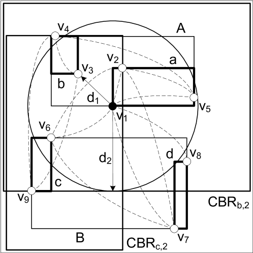
Figure 6: An example of processing a $GSGQ_{rkNN}$ $Q_{gs}=(v_{1},r3NN,2)$.

Algorithm 3 presents the details of processing a $GSGQ$ _rkNN based on an SaR-tree or SaR*-tree. A set $\widetilde{W}$ is used to store the currently visited users and initialized as $\{v\}$. The entries in $H$ are visited in ascending order of $d_{e}$. If a visited entry $e$ is not a leaf entry, it will be further explored and its child entries with $c_{e^{\prime}}\geq c$ are inserted into $H$ (Lines 7-10); otherwise, we get its corresponding user $u$ (Line 12) and proceed with the following steps. If $c_{u}<c$, it means $u$ cannot be a result user. Thus, we simply ignore it and continue checking the next entry of $H$. On the other hand, if $c_{u}\geq c$, $u$ is added into the candidate set $\widetilde{W}$ (Lines 13-14). Then, we compute the maximum $c$-core, denoted as $W^{\prime}$, in the subgraph formed by $\widetilde{W}$ (Line 15). If $|W^{\prime}|\geq k+1$ and $v\in W^{\prime}$, $W^{\prime}-\{v\}$ is the result (Line 16-17); otherwise, the above procedure is continued until the result is found or shown to be non-existent. Theorem 5.3 proves the correctness of Algorithm 3 and its superiority to the baseline accessing model.

Algorithm 3 Processing $GSGQ_{rkNN}$

0:  LBSN $G=(V,E)$, $Q_{gs}=(v,rkNN,c)$

0:  Result of $Q_{gs}$ProGSGQrKNN($G$, $Q_{gs}$)

1:  if $c_{v}<c$ then

2:    return $\phi$;

3:  end if

4:  $\widetilde{W}=\{v\}$;

5:  Initialize $H$ with the entries of the root node;

6:  while $H\neq\phi$ do

7:    Pop the first entry $e$ from $H$;

8:    if $e$ is not a leaf entry then

9:       for each child entry $e^{\prime}$ of $e$ do

10:         if $c_{e^{\prime}}\geq c$ then

11:            Compute $d_{e^{\prime}}$ and put $e^{\prime}$ into $H$;

12:         end if

13:       end for

14:    else

15:       Get the corresponding user $u$ of $e$;

16:       if $c_{u}\geq c$ then

17:         $\widetilde{W}=\widetilde{W}\cup\{u\}$;

18:         if the first entry $e^{\prime}$ in $H$ has $d_{e^{\prime}}>d_{e}$ then

19:            Compute the maximum $c$-core $W^{\prime}$ in $\widetilde{W}$;

20:            if $|W^{\prime}|\geq k+1$ and $v\in W^{\prime}$ then

21:              return $W^{\prime}-\{v\}$;

22:            end if

23:         end if

24:       end if

25:    end if

26:  end while

27:  return $\phi$;

Theorem 5.3

For a $GSGQ_{rkNN}$ $Q_{gs}=(v,rkNN,c)$, Algorithm 3 generates the result of $Q_{gs}$. Moreover, it checks equal or less users than that of the baseline accessing model based on $d(v,MBR_{e})$.

Proof

Let $W$ be the user set returned by Algorithm 3. and user $u^{\prime}=\arg_{u\in W}{\max{d(v,u)}}$. Suppose another user set $W^{\prime}$, $W^{\prime}\neq W$, is the result. Then, it should be either 1) $d_{max}(v,W^{\prime})<d_{max}(v,$$W)$ or 2) $d_{max}(v,W^{\prime})=d_{max}(v,W)$ and $W\subset W^{\prime}$.

For case 1), consider a user $u\in W^{\prime}$. For any entry $e$ which covers $u$, based on Theorem 5.2, we have $d_{e}\leq d_{max}(v,$ $W^{\prime})<d_{max}(v,W)=d(v,u’)\leq d_{u^{\prime}}$. According to Algorithm 3, a super set of $W^{\prime}$, denoted as $W^{\prime\prime}$, should be checked before getting $W$ and $G[W^{\prime\prime}\cup\{v\}]$ does not contain a $c$-core of size no less than $k+1$ covering $v$. Then, $W^{\prime}$ cannot be the result, which is contradictory to the assumption.

For case 2), consider a user $u\in W^{\prime}$ and $u\notin W$. According to Algorithm 3, there is a any entry $e$ which covers $u$ and $d_{e}>d_{u’}$. Based on Theorem 5.2, we have $d_{max}(v,W^{\prime})\geq d_{e}>d_{u^{\prime}}\geq d(v,u’)=d_{max}(v,W)$, which is contradictory to the assumption $d_{max}(v,W^{\prime})=d_{max}(v,W)$.

To conclude, $W$ is the result of $Q_{gs}$.

Let $S$ and $S^{\prime}$ be the entries explored by Algorithm 3 and by the baseline accessing model based on $d(v,MBR_{e})$, respectively, for finding the result set $W$. Based on Theorem 5.2, for any entry $e\in S$, we have $d_{e}\leq d_{max}(v,W)$ (if not, $e$ will not be further explored since all the users of $W$ have been accessed and the result set $W$ has been found). Considering that $S^{\prime}=\{e|d(v,MBR_{e})\leq d_{max}(v,W)\}$, then $S\subseteq\{e|e\in S^{\prime}\wedge d_{in}(v,CBR_{e,c})\leq d_{max}(v,W)\}\subseteq S^{\prime}$. It means $S$ contains equal or less users than that of $S^{\prime}$.

Recall the example in Fig. 6. When applying Algorithm 3 to process $Q_{gs}=(v_{1},r3NN,2)$, the access order of the users is $v_{2}$, $v_{6}$, $v_{5}$, $v_{3}$, $v_{4}$, $v_{9}$ and $v_{7}$. The result can be obtained by accessing the first $3$ users. In contrast, the baseline algorithm based on R-tree accesses the users in the order of $v_{2}$, $v_{3}$, $v_{6}$, $v_{5}$, $v_{4}$, $v_{8}$, $v_{9}$, and $v_{7}$. Then, $4$ users are accessed and processed. Obviously, by reorganizing the access order of entries, Algorithm 3 processes $GSGQ_{rknn}$ more efficiently.

5.3 GSGQ with Strict $k$NN Constraint

For a $GSGQ_{kNN}$ $Q_{gs}=(v,kNN,c)$, we adopt the same processing framework as in Algorithm 3. However, when a valid $W^{\prime}$ is found for $GSGQ_{rkNN}$ at Line 16, more steps will be needed to obtain the result of $GSGQ_{kNN}$. Let $W^{\prime}$ be the maximum $c$-core formed by the set of currently visited users $\widetilde{W}$. Only if $|W^{\prime}|\geq k+1$ and $v\in W^{\prime}$, it is possible to find a $c$-core of size $k+1$ in $\widetilde{W}$ that contains $v$. Moreover, such a $c$-core must be a subset of $W^{\prime}$. Thus, we invoke a function FindExactkNN to check all user sets of size $k+1$ that contain $v$ in $W^{\prime}$. If such a user set $W^{\prime\prime}$ is found, $W^{\prime\prime}-\{v\}$ is the result of $Q_{gs}$; otherwise, the above procedure is repeated when Algorithm 3 continues to find the next candidate $W^{\prime}$.

In-Memory Optimizations. The above processing framework provides optimized node access on SaR-trees for $GSGQ$ _kNN. However, due to the NP-hardness of $GSGQ_{kNN}$, the in-memory processing function FindExactkNN also has a great impact on the performance of the algorithm. A naive idea of checking all possible combinations of the user sets costs up to exponential time complexity of $k$. In this subsection, we single out this problem to optimize the FindExactkNN function by designing two pruning strategies.

Algorithm 4 details the optimized FindExactkNN, which employs a branch-and-bound method and expands the source user set $S$ from the candidate user set $U$. At the beginning, $S$ and $U$ are initialized as $\{v,u\}$ and $W^{\prime}-\{v,u\}$ ($u$ denotes the newly accessed user in Algorithm 3), respectively. Note that if a result $W^{\prime\prime}$ exists in $W^{\prime}$, $W^{\prime\prime}$ must contain $u$, because it has been proved that $W^{\prime}-\{u\}$ does not contain a result. During the processing, two major pruning strategies, namely, core-decomposition based pruning (Lines 6-11, 16-20) and $k$-plex based pruning (Lines 5, 12), are applied.

1) Core-Decomposition based Pruning: Based on the definition of $c$-core, we can observe that if the current source user set $S^{\prime}$ can be expanded to a $c$-core of size $k+1$, it must be contained by the maximum $c$-core of $U^{\prime}\cup S^{\prime}$, where $U^{\prime}$ denotes the set of remaining candidate users. Therefore, we conduct a core-decomposition on $U^{\prime}\cup S^{\prime}$ before further exploration. If a user of $S^{\prime}$ has a core number smaller than $c$ in $U^{\prime}\cup S^{\prime}$, $S^{\prime}$ cannot be expanded to a result from the candidate user set $U^{\prime}$ and thus we can safely stop further exploration. In addition, if the maximum $c$-core in $U^{\prime}\cup S^{\prime}$ contains $S^{\prime}$ and has size $k+1$, it is the result of $GSGQ_{kNN}$ and the whole processing terminates. Otherwise, further exploration on the maximum $c$-core of $U^{\prime}\cup S^{\prime}$ is required. Finally, if $S^{\prime}$ cannot be expanded to a $c$-core of size $k+1$, we roll back to explore $S$ and the remaining $U$. Similarly, we compute the maximum $c$-core $W^{\prime}$ of $S\cup U$. If $|W^{\prime}|\geq k+1$ and $S\subseteq W^{\prime}$, $S$ could be expanded to the result from $U=W^{\prime}-S$ and further exploration is applied; otherwise, no result can be found.

2) $k$-plex based Pruning: One major challenge of the $c$-core problem is that it does not preserve locality, that is, if $W$ is a $c$-core, adding or dropping some users from $W$ no longer retains it as a $c$-core. As a workaround, we transfer the problem to a dual $\bar{c}$-plex problem balas (which preserves the locality property) by adding some constraint. Simply speaking, a $\bar{c}$-plex $W\subseteq V$ is a set such that $\delta(G[W])\geq|W|-\bar{c}$.

Since a $c$-core of size $k+1$ is also a $(k+1-c)$-plex, we seek to find a $(k+1-c)$-plex of size $k+1$ to achieve further pruning. $\bar{c}$-plex preserves the locality property because if $W$ is a $\bar{c}$-plex, dropping some users can still make it a $\bar{c}$-plex. In other words, if the maximum $(k+1-c)$-plex in $U^{\prime}\cup S^{\prime}$ has a size no less than $k+1$, it is certain that a $(k+1-c)$-plex of size $k+1$ can be found; otherwise, such a $(k+1-c)$-plex cannot be found. Moveover, $(k+1-c)$-plex is more constrained than $c$-core because the size of the maximum $(k+1-c)$-plex is always no larger than that of the maximum $c$-core of size no smaller than $k+1$.

Algorithm 4 Finding $c$-core of size $k+1$

0:  User set $U$ and $S$, $c$, $k$

0:  $c$-core $W$ FindExactkNN($U$, $S$, $c$, $k$)

1:  if $|S|=k+1$ then

2:    return $S$;

3:  end if

4:  while $U\neq\phi$ do

5:    $S^{\prime}=S\cup\{u\}$, $U=U-\{u\}$ for some $u\in U$;

6:    $U^{\prime}=\{u\in U:S^{\prime}\cup\{u\}$ is a $(k+1-c)$-plex $\}$;

7:    Compute the maximum $c$-core $W^{\prime}$ of $U^{\prime}\cup S^{\prime}$;

8:    if $|W^{\prime}|\geq k+1$ and $S^{\prime}\subseteq W^{\prime}$ then

9:       if $|W^{\prime}|=k+1$ then

10:         return $W^{\prime}$;

11:       else

12:         $U^{\prime}=W^{\prime}-S^{\prime}$;

13:         if $B_{p}(G[U^{\prime}\cup S^{\prime}])\geq k+1$ then

14:            $W^{\prime\prime}$ = FindExactkNN($U^{\prime}$, $S^{\prime}$, $c$, $k$);

15:            if $W^{\prime\prime}\neq\phi$ then

16:              return $W^{\prime\prime}$;

17:            end if

18:         end if

19:       end if

20:    end if

21:    Compute the maximum $c$-core $W^{\prime}$ of $S\cup U$;

22:    if $|W^{\prime}|\geq k+1$ and $S\subseteq W^{\prime}$ then

23:       $U=W^{\prime}-S$;

24:    else

25:       break;

26:    end if

27:  end while

28:  return $\phi$;

The properties of $(k+1-c)$-plex can be used to devise powerful pruning strategies in processing $GSGQ_{kNN}$. First, we prune those users in $U$ who cannot expand the source user set $S^{\prime}$ to a $(k+1-c)$-plex. This pruning is implemented in Line 5 of Algorithm 4. Second, we estimate the size of a maximum $(k+1-c)$-plex to provide further pruning. Some theoretic bounds on it have been proposed in the literature. In this paper, we adopt the result of mcclosky and compute an upper bound $B$ on the size of a maximum $(k+1-c)$-plex in a graph $G$ as,

$$B_{p}(G)=min_{i=1,\ldots,p}\{\frac{1}{i}B(C^{i}_{1},\ldots,C^{i}_{m_{i}})\},$$ (2)

and

$$B(C^{i}_{1},\ldots,C^{i}_{m_{i}})= \sum_{j=1}^{m_{i}}min\{2\bar{c}-2+\bar{c}\ mod\ 2,\bar{c}+a_{i,j},$$

$$\Delta(G[C^{i}_{j}])+\bar{c},|C^{i}_{j}|\},$$

where $\bar{c}=k+1-c$, $C^{i}_{1},\ldots,C^{i}_{m_{i}}$ are co-$\bar{c}$-plexes mcclosky in which every vertex of $V$ appears exactly $i$ times, $a_{i,j}=max\{n:|\{v|v\in V\wedge deg_{G}(v)\geq n\}|\geq\bar{c}+l\}$ for each $C^{i}_{j}$, and $p$ is a parameter to limit the iterations of computing.

Fig. 7 shows the steps of both the basic and optimized version of function FindExactkNN where user set $W^{\prime}=\{v_{1},v_{2},v_{3},v_{6},v_{9},v_{8},$ $v_{4},v_{7}\}$ and $Q_{gs}=(v_{1},3NN,2)$. In the optimized procedure, each step shows the investigated source user set $S^{\prime}$ and the candidate set $U^{\prime}$ after filtering. For example, in the first step, we try to check $S^{\prime}=\{v_{1},v_{7},v_{4}\}$ and $U^{\prime}=\{v_{2},v_{3},v_{6},v_{8},v_{9}\}$. After filtering $U^{\prime}$ via Line 5 of Algorithm 4, we can get $U^{\prime}=\{v_{2},v_{6},v_{8},v_{9}\}$. Since the maximum $2$-core of $U^{\prime}\cup S^{\prime}$ only has size $3$, no $2$-core of size $4$ can be found in $U^{\prime}\cup S^{\prime}$. Thus, all the combinations of these users can be ignored. A similar case can be found in the second step when $S^{\prime}=\{v_{1},v_{7},v_{9}\}$. In the third step, we can get the upper bound of the size of the maximum $2$-plex in $U^{\prime}\cup S^{\prime}$ as $3$ by computing $B_{2}(G[U^{\prime}\cup S^{\prime}])$. Thus, $U^{\prime}\cup S^{\prime}$ does not contain a $2$-core of size $4$. We can stop searching here because no user is filtered from $U^{\prime}$ in the last step, which means all the combinations are covered. We can see that the optimized function FindExactkNN effectively prunes unnecessary explorations and saves significant computation cost.

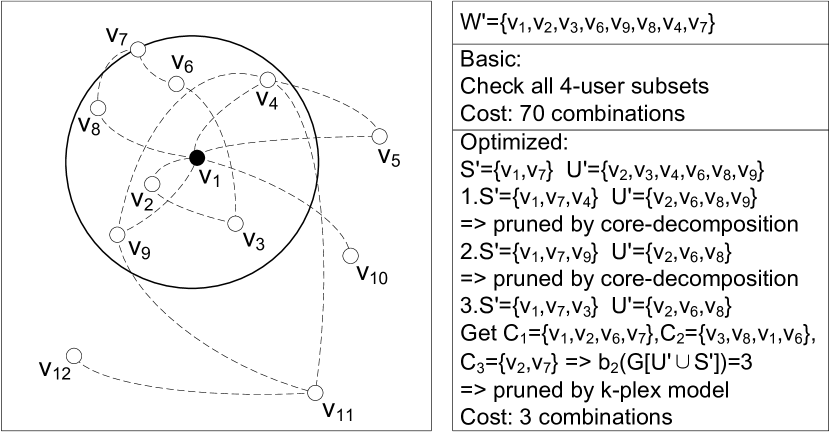
Figure 7: Exemplary procedures of the original and optimized function FindExactkNN when $W^{\prime}=\{v_{1},v_{2},v_{3},v_{6},v_{9},v_{8},v_{4},v_{7}\}$ for $GSGQ_{kNN}$ $Q_{gs}=(v_{1},3NN,2)$. The entries are omitted here because they are not related to function FindExactkNN.

6 Update of SaR-trees

The SaR-trees, once built, can be used as underlying structures for efficient GSGQ processing with generic spatial constraints. It is particularly favorable for applications where both social relations and user locations (e.g., home addresses) are stable. However, for other applications where users may regularly change their locations and social relations, efficient update of the SaR-trees is required. This is challenging because an update of a user affects not only her own CBR but also those of others. In this section, we propose a lazy update approach tailored for SaR-trees that strikes a balance between update efficiency and effectiveness of GSGQ processing.

6.1 Lazy Update in SaR-trees

An update from user $v\in G$ means either her location changes from $p_{v}$ to $p^{\prime}_{v}$ or her social relation $N_{G}(v)$ changes. However, not all changes lead to the update of CBRs. The following two rules show the location and social conditions on which CBRs might need updates.

Update Rule 1

Location update. A $CBR_{u,c}$ might become invalid only if there exists some user $v$ such that $c\leq c_{v}$, $p_{v}\notin CBR_{u,c}$, and $p^{\prime}_{v}\in CBR_{u,c}$.

Update Rule 2

Social updates. A $CBR_{u,c}$ might become invalid only if there exist two users $v,v^{\prime}$ such that edge $vv^{\prime}$ is newly added, $min\{c_{v},c_{v^{\prime}}\}\geq c$ and $\{p_{v},p_{v^{\prime}}\}\in CBR_{u,c}$.

To relieve an update procedure from intensive CBR re-computation, we propose a lazy update model for SaR-trees. Particularly, a memo $M$ is introduced to store those accumulated updates which have not been applied on the CBRs of SaR-trees. Fig. 8 illustrates the data structure for the SaR-tree in Fig. 5. A user update is thus handled in three steps. In the first step, the user record is updated, and core-decomposition is performed on $G$ to update the core numbers of users if it is a social update. If the core number of a user $u$ changes, the core numbers of the entries along the path from $u$ to the root are updated. In the second step, the user update is added into $M$. In this figure, user $v_{2}$ adds an edge with $v_{3}$, and the new edge has been inserted to $M$. Similar operation is performed for location updates when a user moves into other users’ CBRs. In the third step, when the size of $M$ reaches a threshold, named the Batch Update Size, a batch update is applied on the CBRs of SaR-trees. This calls for re-computation of all affected CBRs in $M$.

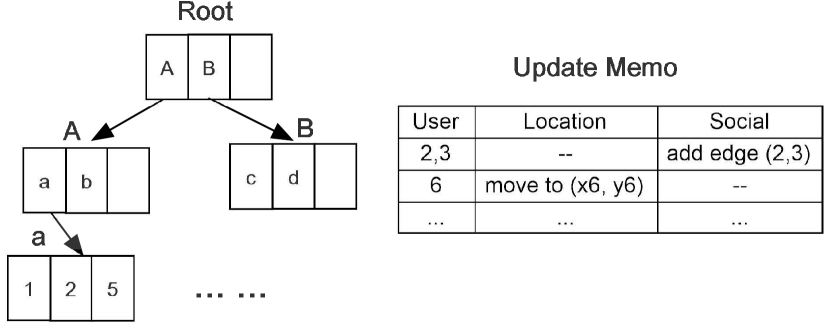
Figure 8: Lazy Update and Update Memo

To facilitate CBR updates, an R-tree is built on the CBRs of users. By a point containment query on this R-tree, we can find the CBRs that cover the latest location of an updated user. The retrieved CBRs are then filtered based on Update Rule 1 and Update Rule 2. For the remaining CBRs, we first determine their validity by computing the core numbers of the corresponding users in the subgraphs formed by the users inside the CBRs. Then, each invalid CBR is recomputed by applying Algorithm 1 and its update is propagated to the root along the SaR-tree path.

6.2 GSGQ Processing with Update-Memo on SaR-trees

With an update-memo $M$, GSGQ processing algorithms on SaR-trees need to be revised for correctness as some CBRs may be invalid. In the following, we outline the major changes of the processing algorithms for different GSGQs.

$GSGQ_{range}$ processing. To revise Algorithm 2, the CBRs will no longer be used to prune entries when traversing the SaR-tree. As a result, the priority queue $H$ is composed of a number of leaf entries, each corresponding to a user with core number equal to or larger than $c$ inside $range$. As such, for each user $u$ in $H$ s.t. $range\subset CBR_{u,c}$, we check the other users in $H$ located inside range: if some other user has updates in $M$ which might invalidate $CBR_{u,c}$ according to Update Rule 1 or 2, we keep $u$ in $H$; otherwise, $u$ is pruned from $H$. In the end, if the query issuer $v$ is pruned from $H$, there will be no result; otherwise, we obtain the result from $H$ as Algorithm 2 does.

$GSGQ_{rkNN}$ (or $GSGQ_{kNN}$) processing. To revise Algorithm 3, we still use the second priority queue $H^{\prime}$ to store the entries of $H$ in ascending order of their minimal distances to $v$. When putting an entry $e$ into $H$, if $d_{in}(v,CBR_{e,c})$ $>d(v,MBR_{e})$, we need to verify the validity of $CBR_{e,c}$. For a non-leaf entry $e$, we simply set $d_{e}=d(v,MBR_{e})$ to avoid the validating cost. For a leaf entry $e$, let $u$ be the corresponding user. We retrieve all users with shorter distances to the query issuer $v$ than $d_{in}(v,CBR_{e,c})$ by exploring $H^{\prime}$, denoted as $U$. Then, we filter out the users in $U$ who has no update in $M$ or cannot invalidate $CBR_{e,c}$ according to Update Rule 1 or 2. If $U$ is not empty, $d_{in}(v,CBR_{e,c})$ is updated as $min_{u^{\prime}\in U}d(v,u^{\prime})$. It is easy to verify that if $p_{u}\in\odot(v,min_{u^{\prime}\in U}d(v,u^{\prime}))$, any user group with $u$ inside $\odot(v,min_{u^{\prime}\in U}d(v,u^{\prime}))$ cannot be a $c$-core. This guarantees the correctness of the algorithm.

7 Performance Evaluation

In this section, we evaluate the proposed methods on three real datasets, namely, Gowalla, Dianping, and Twitter-2010, and investigate the impact of various parameters. The code is written in C++ and compiled by GNU gcc x64 4.5.2. All the experiments are performed on a Dell R430 server with dual Intel Xeon E5-2620 CPU and 64GB RAM, running GNU/Ubuntu Linux 64-bit 14.04 LTS.

7.1 Experimental Setting

The Gowalla dataset was collected from the location-based social network Gowalla (available on http://snap.stan-ford.edu/data/loc-gowalla.html), the Dianping dataset was crawled by us from a Chinese restaurant review site (available on https://goo.gl/uUV4Wg), and the Twitter-2010 dataset is from the social network Twitter (available on http://law.di.unimi.it/webdata/twitter-2010/). For the Gowalla dataset and the Dianping dataset, we remove the users with no check-ins and select the first check-in position of each user as his/her location. As a result, the preprocessed Gowalla dataset has 107,092 nodes (users) and 456,830 edges (friend relations), while the preprocessed Dianping dataset has 2,673,970 nodes and 922,977 edges. In comparison, the Twitter-2010 dataset is much bigger, with 41,652,098 nodes and 684,500,219 edges. The locations of the users in Twitter-2010 are randomly generated with a uniform distribution. For both datasets, we normalize the location data into a unit space [0,1] x [0, 1].

We implement four indexes for performance evaluation, namely, R-tree, C-imbedded R-tree, SaR-tree, and SaR*-tree. The C-imbedded R-tree is built on top of an R-tree and additionally stores the core numbers of the index entries. The average CPU time of constructing a user CBR in the latter two trees is less than $100$ ms for Gowalla and Dianping, and $50$ ms for Twitter-2010. The sizes of SaR-trees are 15.5MB for Gowalla, 257MB for Dianping and 2.1GB for Twitter-2010. The index construction time is less than 1 minute for Gowalla and Dianping, and 1.3 hours for Twitter-2010. The corresponding GSGQ processing methods on these indexes are denoted as BR (baseline R-tree), CR, SaR and SaR*, respectively. CR enhances BR by pruning those nodes whose core numbers cannot satisfy the minimum degree constraint $c$ in query processing.

Table 1: System parameter settings

Parameter	Value	Parameter	Value
$c$	$1-5$	$r$	$0.002-0.05$
$k$	$10-250$	Page size	4KB
Page acc. time	2ms
Gowalla
User #	$107,092$	Edge #	$456,830$
Max degree	$9,967$	Avg. degree	$9.177$
Max core num.	$43$	Avg. core num.	$4.839$
Dataset size	27.2MB
Dianping
User #	$2,673,970$	Edge #	$922,977$
Max degree	$11423$	Avg. degree	$5.184$
Max core num.	$24$	Avg. core num.	$2.741$
Data size	162M
Twitter-2010
User #	$41,652,098$	Edge #	$684,500,219$
Max degree	$1,405,986$	Avg. degree	$30.453$
Max core num.	$2,059$	Avg. core num.	$14.692$
Dataset size	29.7GB

To have a fair comparison, we implement CR, SaR, and SaR* by coupling extra pages with each index node to store the information of core numbers (for CR) or CBRs (for SaR and SaR*). These extra pages are called coupled nodes. To compare the performance of different methods, we mainly use two metrics, namely, the page access cost and the query running time. The former includes the page accesses of index nodes, coupled nodes, and user data. On the other hand, the query running time measures the actual clock time to process a GSGQ, including the CPU time and the I/O time. In the experiments, no cache is used for GSGQ processing and the page access time is set as $2$ ms per page access. Each test ran a set of 1,000 randomly generated GSGQs and we report the average performance.

Three types of queries, namely, $GSGQ_{range}$, $GSGQ_{rkNN}$, and $GSGQ_{kNN}$, are tested. For $GSGQ_{range}$, the range $r$ is defined as a square centered at the location of the query issuer. In the sequel, we use the edge length to represent $r$, which is set at $0.002$ for Gowalla and Dianping, and $0.05$ for Twitter-2010 by default. For $GSGQ_{rkNN}$ and $GSGQ_{kNN}$, $k$ is selected from $10$ to $250$, which represents large-scale time-consuming queries for real-life social applications, e.g., the marketing example shown in Section 1. Finally, the minimum degree constraint $c$ is selected from $1$ to $5$. Table 1 summarizes the major parameters and their values used in the experiments, where the average degree only counts connected nodes.

7.2 Overall Performance

Table 2 shows the average minimum degree of the result groups for three different query semantics on Gowalla, where $kNN$ denotes a classic $k$-nearest-neighbor query and $SSGQ$ denotes the socio-spatial group query proposed in yang12 . As expected, GSGQ always retrieves the groups that satisfy the minimum degree constraints, while the other two queries have a minimum degree of close to zero. This justifies the improved social constraint introduced by GSGQ.

Table 2: Minimum degree of the result group given $k=50$ on Gowalla.

Query	$\rho$
	1	2	3	4	5
$kNN$	0	0	0	0	0
$SSGQ(p=\rho)$	0.05	0.08	0.11	0.16	0.21
$GSGQ_{rkNN}(c=\rho)$	1	2	3	4	5

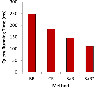
(a) $GSGQ_{range}$ (r=0.002, c=4)

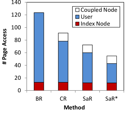
(b) $GSGQ_{range}$ (r=0.002, c=4)

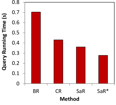
(c) $GSGQ_{rkNN}$ (k=100, c=4)

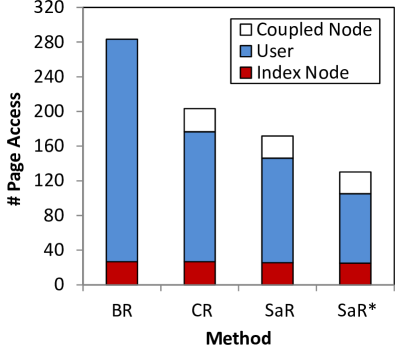
(d) $GSGQ_{rkNN}$ (k=100, c=4)

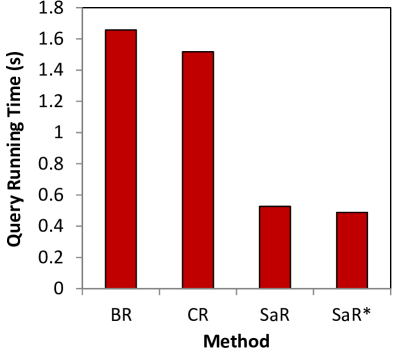
(e) $GSGQ_{kNN}$ (k=100, c=3)

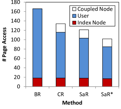
(f) $GSGQ_{kNN}$ (k=100, c=3)

Figure 9: Overall performance comparison on Gowalla.

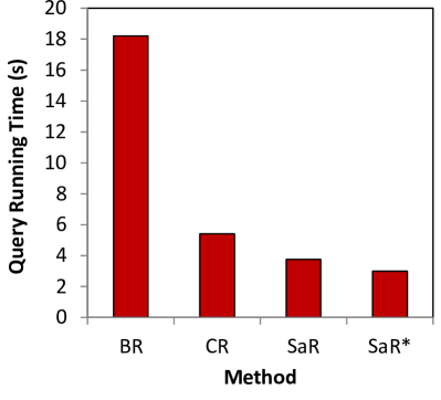
(a) $GSGQ_{range}$ (r=0.002, c=4)

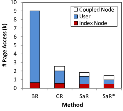
(b) $GSGQ_{range}$ (r=0.002, c=4)

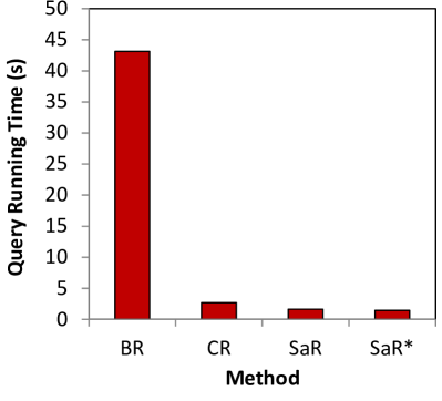
(c) $GSGQ_{rkNN}$ (k=100, c=4)

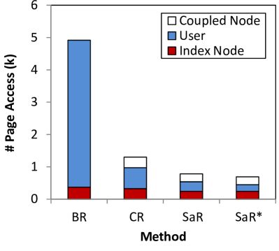
(d) $GSGQ_{rkNN}$ (k=100, c=4)

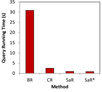
(e) $GSGQ_{kNN}$ (k=30, c=8)

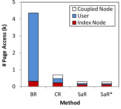
(f) $GSGQ_{kNN}$ (k=30, c=8)

Figure 10: Overall performance comparison on Dianping.

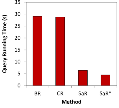
(a) $GSGQ_{range}$ (r=0.05, c=2)

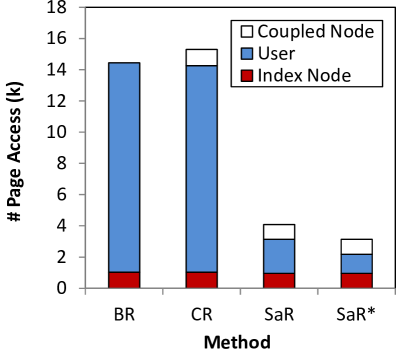
(b) $GSGQ_{range}$ (r=0.05, c=2)

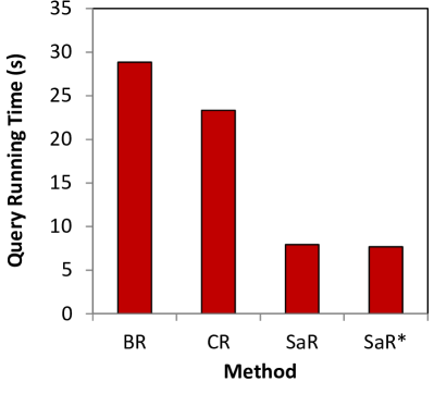
(c) $GSGQ_{rkNN}$ (k=20, c=2)

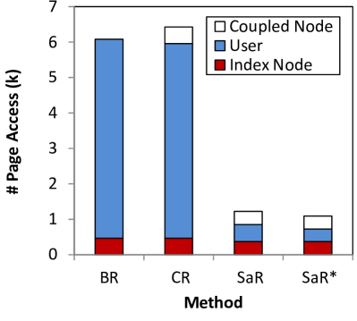
(d) $GSGQ_{rkNN}$ (k=20, c=2)

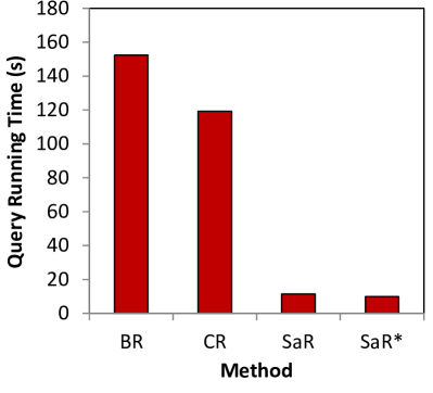
(e) $GSGQ_{kNN}$ (k=20, c=2)

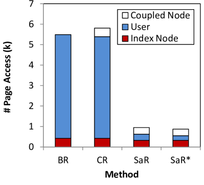
(f) $GSGQ_{kNN}$ (k=20, c=2)

Figure 11: Overall performance comparison on Twitter-2010.

Fig. 9, Fig. 10 and Fig. 11 show the overall performance of the GSGQ methods under three different queries on Gowalla, Dianping and Twitter-2010, respectively. Generally, SaR and SaR* achieve significant improvement over BR and CR in all tested cases. Take Twitter-2010 as an example. For $GSGQ_{range}$, SaR and SaR* outperform BR and CR by $77.9\%-77.6\%$ and $84.5\%-84.3\%$ in terms of the query running time (see Fig. 11(a)). This is mainly due to the savings in accessing the user data as shown in Fig. 11(b). It is interesting to note that CR incurs an even higher page access cost than BR because of the week pruning power of the core numbers for large social networks and additional accesses on the coupled nodes. More specifically, SaR and SaR* check much fewer users (around 2,946 users) than CR (around 103,060 users) and BR (around 85,686 users) to derive the results. SaR* further reduces the page accesses to 3,135 compared to SaR (4,089), CR (15,293), and BR (14,436). All the results exhibit the high pruning power of CBRs for $GSGQ_{range}$ processing.

For $GSGQ_{rkNN}$, SaR and SaR* achieve similar improvement over BR and CR in terms of the query running time and the page access cost (see Fig. 11(c) and Fig. 11(d)). They access much less users in query processing. Specifically, SaR and SaR* only check $3.0\%$ users of BR and $3.6\%$ users of CR. For $GSGQ_{kNN}$, the improvement on query running time is even more higher for SaR and SaR* because of the in-memory optimizations (see Fig. 11(e)). That is, compared to BR (resp. CR), SaR and SaR* save $92.5\%$ (resp. $90.4\%$) and $93.5\%$ (resp. $91.7\%$) of query running time. This indicates that by optimizing the accessing order of the entries based on the CBRs, a greater performance improvement can be achieved.

Finally, comparing Fig. 11 to Fig. 9 and Fig. 10, we can see that our methods gain a higher improvement over CR on Twitter-2010 than on Gowalla and Dianping. This is because Twitter-2010 has a denser social network and more diverse locations, thus limiting the pruning power of the core numbers and making it harder to process a GSGQ. As a further investigation on the impact of the social graph with different sizes and density, we choose subsets of users in Twitter-2010 from 5M to 40M, and Table 3 shows the average degrees and core numbers of these induced subgraphs. Fig. 12 plots the performance comparison of $GSGQ_{rkNN}$ queries on these social graphs. We can see that as the graph density grows, the performance gap between CR and SaR/SaR* increases, because less pruning power can be obtained from the core numbers. Compared to BR, SaR and SaR* retain the pruning power and reduce the page access by roughly the same ratio. The query running time of BR increases on the graph of 40M users because there is a jump of the graph density from 20M users to 40M users and thus less time saving can be achieved in the in-memory processing. To conclude, the pruning power of SaR and SaR*, mainly contributed by the social relations in CBRs, benefits more from larger and denser social networks.

Table 3: Density of Twitter-2010 with different user #.

User # (m)	5	10	20	40
Avg. degree	1.957	2.613	4.783	28.556
Avg. core num.	1.066	1.461	2.463	14.480

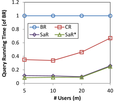
(a) $GSGQ_{rkNN}$ (k=10, c=2)

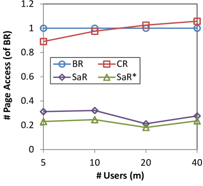
(b) $GSGQ_{rkNN}$ (k=10, c=2)

Figure 12: Overall performance comparison on Twitter-2010 with different user #.

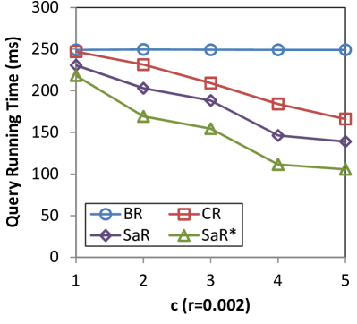
(a) Gowalla

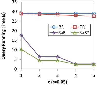
(b) Twitter-2010

Figure 13: Query running time of the methods for $GSGQ_{range}$ queries with different $c$ settings.

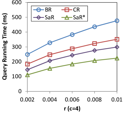
(a) Gowalla

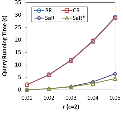
(b) Twitter-2010

Figure 14: Query running time of the methods for $GSGQ_{range}$ queries with different $r$ settings.

7.3 $GSGQ_{range}$ Processing

For a $GSGQ_{range}$ $Q_{gs}=(v,r,c)$, Fig. 13 shows the performance with different $c$ settings on Gowalla and Twitter-2010. All methods except BR incur shorter query running time for a larger $c$. The performance gap between BR and the other methods increases as $c$ grows. This is because more users and index nodes can be pruned in CR, SaR, and SaR* for a large $c$. SaR and SaR* outperform CR in all cases. The improvement reduces a little at $c=3$ and $c=5$ because only approximate CBRs (corresponding to $c=2$ and $c=4$, respectively) are used for query processing in these cases (recall that only the CBRs with respect to exponential minimum degree constraints are stored). Moreover, SaR* benefits more from the index than CR and SaR, as it groups the users based on both spatial and social closenesses, making the pruning of index nodes and user pages more powerful. As for various settings of query range $r$ (see Fig. 14), the performance of all methods degrades when $r$ grows, because more users within the range need to be checked. In terms of query running time, SaR and SaR* perform much better than the other two methods. Moreover, SaR* has the best performance and thus is the most favorable approach.

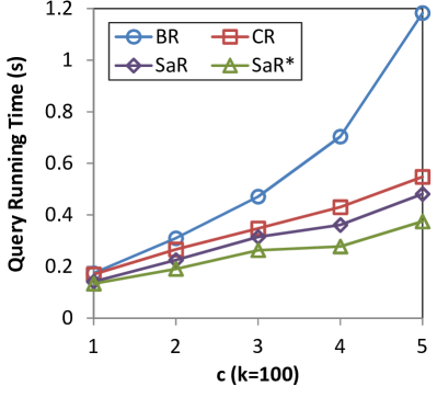
(a) Gowalla

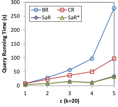
(b) Twitter-2010

Figure 15: Query running time of the methods for $GSGQ_{rkNN}$ queries with different $c$ settings.

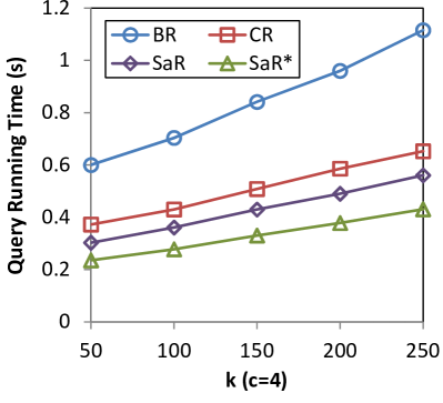
(a) Gowalla

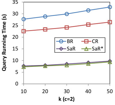
(b) Twitter-2010

Figure 16: Query running time of the methods for $GSGQ_{rkNN}$ queries with different $k$ settings.

7.4 $GSGQ_{rkNN}$ Processing

This subsection investigates the performance of the methods for $GSGQ_{rkNN}$ under various $c$ and $k$ settings. As we observed similar performance trends for $GSGQ_{kNN}$ under these settings, we omit the details on $GSGQ_{kNN}$ here.

For a $GSGQ_{rkNN}$ $Q_{gs}=(v,rkNN,c)$, Fig. 15 shows the performance with different $c$ settings on Gowalla and Twitter-2010. All methods incur higher query running time for a larger $c$. This is because a large $c$ tightens the social constraint of $GSGQ_{rkNN}$ and thus more users need to be visited. Similar to $GSGQ_{range}$, the performance gaps between SaR* and the other two methods increase as $c$ grows. For a larger $c$, the candidate users for $GSGQ_{rkNN}$ processing tend to share similar CBRs. Thus, the social-aware user organization of SaR* can effectively reduce the page accesses.

Fig. 16 shows the performance with different $k$ settings on Gowalla and Twitter-2010. Compared to $c$, the increment of $k$ causes only a moderate increase in cost. SaR and SaR* beat BR and CR for all $k$ settings and the performance gaps become larger as $k$ grows. This implies that the pruning techniques of SaR and SaR* are scalable to large user groups.

Table 4: Average # of updated CBRs w.r.t. batch update size.

Upd. Size ($k$)	1	3	10	30	100	300
Gowalla	13.14	5.71	2.27	1.05	0.45	0.16
Upd. Size ($k$)	10	30	100	300	1000
Twitter-2010	2927.7	1137.3	346.1	115.4	34.6

7.5 Update Performance of SaR-trees

This section investigates the update performance of SaR-trees. We take the locations of user check-ins along the timeline of Gowalla and Twitter-2010 to generate location updates (where the new check-ins for Twitter-2010 are randomly generated with the maximum distance 0.0015 from the last ones) and randomly insert new edges to generate social updates on users. Due to the fact that social updates are relatively infrequent in real social networks lesk , the proportion of social updates is set to $5\%$. We first investigate the effect of batch update size. In general, the average amortized update time decreases as more updates are applied in batch processing. This is mainly because fewer CBRs, on average, are required to update as summarized in Table 4. Fig. 17 (resp. Fig. 18) shows the performance for the $GSGQ_{rkNN}$ queries with default settings under different batch update sizes on Gowalla (resp. Twitter-2010). We can see that the performance of SaR and SaR* degrades as the batch update size grows, which is mainly because more CBRs are invalidated by the updates of $M$ and less pruning power could be achieved (yet still better than BR or CR).

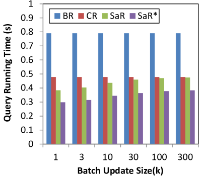
(a) Query Running Time

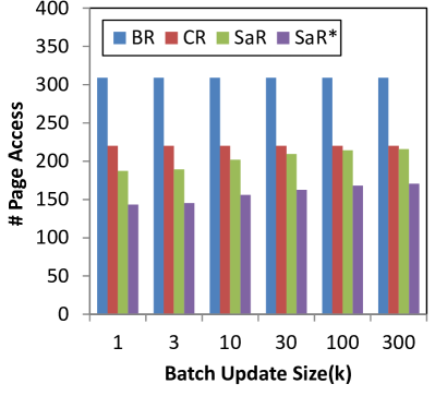
(b) Page Access Cost

Figure 17: The performance of the lazy update model on Gowalla.

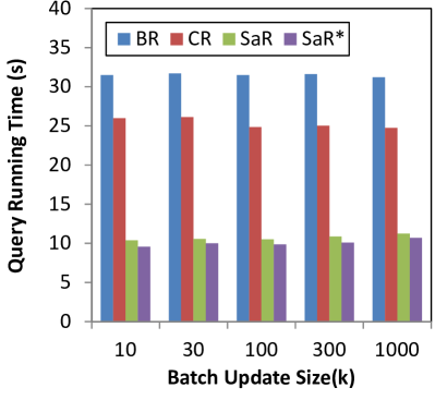
(a) Query Running Time

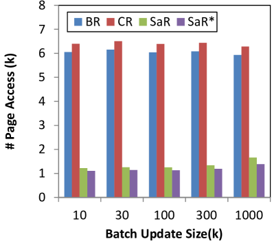
(b) Page Access Cost

Figure 18: The performance of the lazy update model on Twitter-2010.

To further measure the impact of updates on query processing, we generate workloads of mixed update and query requests (i.e., the $GSGQ_{rkNN}$ queries with default settings). Fig. 19(a) shows the throughputs under various query/update ratios (workloads) on Gowalla. SaR* and SaR achieve higher throughputs than CR when the workload has fewer updates, i.e., $q/u>1$ and $10$, respectively, because the performance gain from query processing can compensate for the additional CBR update cost. Fig. 19(b) shows the thoughputs under different batch update sizes on Gowalla. We can see that SaR outperforms CR only for a range of the batch update size. It is because large batch update size leads to obvious performance degradation of SaR for GSGQ processing, making it incapable to compensate for the CBR update cost any more. In comparison, SaR* always achieves the highest throughput. This can also be observed on Twitter-2010, as shown in Fig. 20.

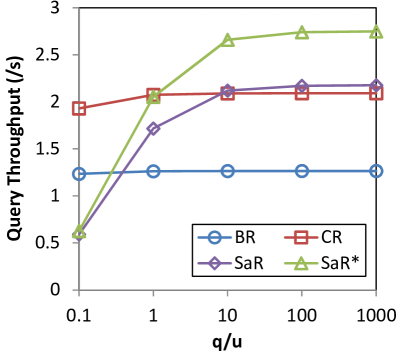
(a) Batch Update Size = $30k$

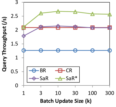
(b) $q/u=10$

Figure 19: The query throughput of the methods on Gowalla.

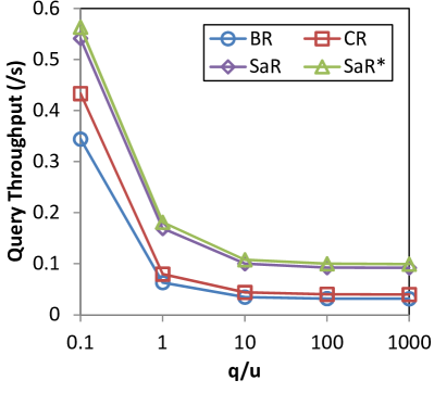
(a) Batch Update Size = $300k$

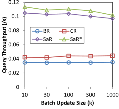
(b) $q/u=10$

Figure 20: The query throughput of the methods on Twitter-2010.

7.6 Case Study: SSGQ vs. GSGQ

We also conducted a case study on the usefulness of GSGQ against SSGQ yang12 . We randomly chose $8$ users from the Gowalla dataset and generated SSGQ and GSGQ kNN results under the following $4$ parameter settings (i.e., $2$ users under each setting): (1) $k=5$, $c=p=1$; (2) $k=5$, $c=p=2$; (3) $k=10$, $c=p=1$; (4) $k=10$, $c=p=2$ . For each user, the SSGQ result is visualized side by side with the GSGQ result in the context of Google Map and social relation of users. 28 participants were invited to give (blind) opinions on which result each user should choose for a group activity. Fig. 21 shows the comparison result. Of all $8$ users except for #2 user, GSGQ is consistently chosen more often than SSGQ queries, and overall in $78$% cases a participant chooses GSGQ results and in only $18$% cases a participant chooses SSGQ results. This case study justifies our motivation of GSGQ as a more useful geo-social group query.

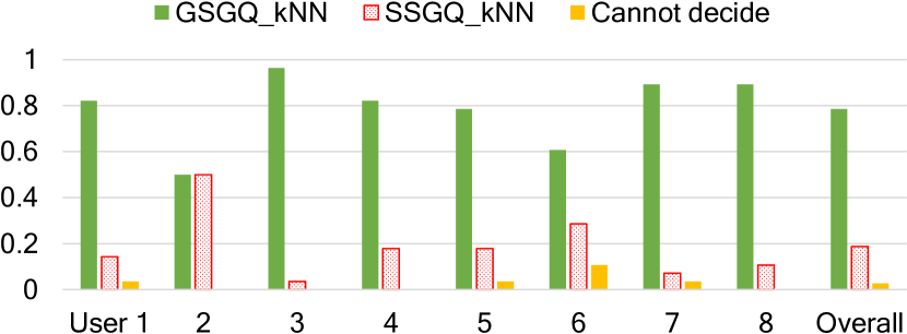
Figure 21: Percentage of Participants’ Choice for Each User

8 Conclusion

This paper has studied geo-social group queries (GSGQs) with minimum acquaintance constraints for large social networking services. Our main contribution is the design of two social-aware index structures, namely SaR-tree and SaR*-tree. Based on them, we have developed efficient algorithms to process various GSGQs, together with a number of optimization techniques. Extensive experiments on real-world datasets demonstrate that our proposed methods substantially outperform the baseline methods based on R-tree under various system settings, and that such GSGQ services are feasible on a commodity server for large user populations. As for future work, we plan to extend GSGQs to incorporate more sophisticated spatial queries such as skyline and distance-based joins.

References

- (1) Nikos Armenatzoglou, Stavros Papadopoulos, and Dimitris Papadias. A general framework for geo-social query processing. In Proc. VLDB, 2013.
- (2) B. Balasundaram, S. Butenko, and I. V. Hicks. Clique relaxations in social network analysis: The maximum k-plex problem. In Operations Research, 2009.
- (3) V. Batagelj and M. Zaversnik. An o(m) algorithm for cores decomposition of networks. In CoRR, 2003.
- (4) Norbert Beckmann, Hans-Peter Kriegel, Ralf Schneider, and Bernhard Seeger. The R*-tree: An efficient and robust access method for points and rectangles. In Proc. SIGMOD, 1990.
- (5) Xin Cao, Gao Cong, Christian S. Jensen, and Beng Chin Ooi. Collective spatial keyword querying. In SIGMOD Conference, 2011.
- (6) James Cheng, Yiping Ke, Shumo Chu, and M. Tamer Ozsu. Efficient core decomposition in massive networks. In Proc. ICDE, 2011.
- (7) Yerach Doytsher, Ben Galon, and Yaron Kanza. Querying geo-social data by bridging spatial networks and social networks. In ACM LBSN, 2010.
- (8) C. Faloutsos, K. McCurley, and A. Tomkins. Fast discovery of connection subgraphs. In KDD, 2004.
- (9) Ian De Felipe, Vagelis Hristidis, and Naphtali Rishe. Keyword search on spatial databases. In Proc. ICDE, 2008.
- (10) Raphael Finkel and J. L. Bentley. Quad trees: A data structure for retrieval on composite keys. In Acta Informatica, 1974.
- (11) S. Fortunato. Community detection in graphs. Physics Reports, 486:3-5:75–174, 2010.
- (12) M. Girvan and M. E. J. Newman. Community structure in social and biological networks. In Proceedings of the National Academy of Sciences of the USA, 2002.
- (13) Antonin Guttman. R-trees: A dynamic index structure for spatial searching. In Proc. SIGMOD, 1984.
- (14) Fei Hao, Shuai Li, Geyong Min, Hee-Cheol Kim, S.S. Yau, and L.T. Yang. An efficient approach to generating location-sensitive recommendations in ad-hoc social network environments. IEEE Transactions on Services Computing, 2015.
- (15) F. Harary and I. C. Ross. A procedure for clique detection using the group matrix. In Sociometry, 1957.
- (16) Osman Khalid, Muhammad Usman Shahid Khan, Samee U. Khan, and Albert Y. Zomaya. OmniSuggest: A ubiquitous cloud based context aware recommendation system for mobile social networks. IEEE Transactions on Services Computing, 2016.
- (17) Jure Leskovec, Lars Backstrom, Ravi Kumar, and Andrew Tomkins. Microscopic evolution of social networks. In KDD, 2008.
- (18) Yafei Li, Rui Chen, Lei Chen, and Jianliang Xu. Towards social-aware ridesharing group query services. IEEE Transactions on Services Computing (TSC), accepted to appear.
- (19) Yafei Li, Rui Chen, Jianliang Xu, Qiao Huang, Haibo Hu, and Byron Choi. Geo-social k-cover qroup queries for collaborative spatial computing. IEEE Transactions on Knowledge and Data Engineering (TKDE), 27(8): 2729-2742, October 2015.
- (20) Weimo Liu, Weiwei Sun, Chunan Chen, Yan Huang, Yinan Jing, and Kunjie Chen. Circle of friend query in geo-social networks. In DASFFA, 2012.
- (21) B. McClosky and I. V. Hicks. Combinatorial algorithms for max k-plex. In Journal of Combinatorial Optimization, 2012.
- (22) H. Moser, R. Niedermeier, and M. Sorge. Algorithms and experiments for clique relaxations-finding maximum s-plexes. In SEA, 2009.
- (23) Dimitris Papadias, Qiongmao Shen, Yufei Tao, and Kyriakos Mouratidis. Group nearest neighbor queries. In ICDE, 2004.
- (24) Roman Schlegel, Chi-Yin Chow, Qiong Huang, and Duncan S. Wong. Privacy-preserving location sharing services for social networks. IEEE Transactions on Service Computing, 2016.
- (25) S. B. Seidman. Network structure and minimum degree. In Social Networks, 1983.
- (26) Jieming Shi, Nikos Mamoulis, Dingming Wu, and David W. Cheung. Density-based place clustering in geo-social networks. In Proc. ACM SIGMOD, 2014.
- (27) Kijung Shin, Tina Eliassi-Rad, and Christos Faloutsos. CoreScope: Graph Mining Using k-Core Analysis - Patterns, Anomalies, and Algorithms. In Proc. IEEE ICDE, 2016.
- (28) M. Sozio and A. Gionis. The community-search problem and how to plan a successful cocktail party. In KDD, 2010.
- (29) Dingming Wu, Man Lung Yiu, Christian S. Jensen, and Gao Cong. Efficient continuously moving top-k spatial keyword query processing. In Proc. ICDE, 2011.
- (30) De-Nian Yang, Yi-Ling Chen, Wang-Chien Lee, and Ming-Syan Chen. On social-temporal group query with acquaintance constraint. In Proc. VLDB, 2011.
- (31) De-Nian Yang, Chih-Ya Shen, Wang-Chien Lee, and Ming-Syan Chen. On socio-spatial group query for location-based social networks. In KDD, 2012.
- (32) Dongxiang Zhang, Yeow Meng Chee, Anirban Mondal, Anthony K. H. Tung, and Masaru Kitsuregawa. Keyword search in spatial databases: Towards searching by document. In Proc. ICDE, 2009.
- (33) Jia-Dong Zhang, Chi-Yin Chow, and Y. Li. iGeoRec: A personalized and efficient geographical location recommendation framework. IEEE Transactions on Services Computing, 2015.
- (34) Jia-Dong Zhang and Chi-Yin Chow. iGSLR: Personalized geo-social location recommendation - A kernel density estimation approach. In Proc. ACM GIS, 2013.