The Black Hole Mass of NGC 4151. II. Stellar Dynamical Measurement from Near-Infrared Integral Field Spectroscopy

Abstract

We present a revised measurement of the mass of the central black hole (${{\mathrm{M}}_{\rm BH}\,}$) in the Seyfert 1 galaxy NGC 4151. The new stellar dynamical mass measurement is derived by applying an axisymmetric orbit-superposition code to near-infrared integral field data obtained using adaptive optics with the Gemini NIFS spectrograph. When our models attempt to fit both the NIFS kinematics and additional low spatial resolution kinematics, our results depend sensitively on how $\chi^{2}$ is computed — probably a consequence of complex bar kinematics that manifest immediately outside the nuclear region. The most robust results are obtained when only the high spatial resolution kinematic constraints in the nuclear region are included in the fit. Our best estimates for the BH mass and $H$-band mass-to-light ratio are ${{\mathrm{M}}_{\rm BH}\,}\sim 3.76\pm 1.15\times 10^{7}~{}{{\mathrm{M}}_{\odot}}$ (1$\sigma$ error) and $\Upsilon_{H}\sim 0.34{\pm 0.03}~{}{{\mathrm{M}}_{\odot}}/{{\mathrm{L}}_{\odot}}$ (3$\sigma$ error), respectively (the quoted errors reflect the model uncertainties). Our BH mass measurement is consistent with estimates from both reverberation mapping ($3.57^{+0.45}_{-0.37}\times~{}10^{7}~{}{{\mathrm{M}}_{\odot}}$) and gas kinematics ($3.0^{+0.75}_{-2.2}\times~{}10^{7}~{}{{\mathrm{M}}_{\odot}}$; 1$\sigma$ errors), and our best-fit mass-to-light ratio is consistent with the photometric estimate of $\Upsilon_{H}=0.4\pm 0.2~{}{{\mathrm{M}}_{\odot}}/{{\mathrm{L}}_{\odot}}$. The NIFS kinematics give a central bulge velocity dispersion $\sigma_{c}=116\pm 3$ ${\mathrm{km\,s^{-1}}}$, bringing this object slightly closer to the M${}_{\rm BH}-\sigma$ relation for quiescent galaxies. Although NGC 4151 is one of only a few Seyfert 1 galaxies in which it is possible to obtain a direct dynamical BH mass measurement — and thus, an independent calibration of the reverberation mapping mass scale — the complex bar kinematics makes it less than ideally suited for this purpose.

1. INTRODUCTION

Long before the development of General Relativity, John Michell wondered about the gravitational influence of objects on the light they emit, and how one might go about finding objects so dense that light could not escape their surfaces. “[I]f any other luminous bodies should happen to revolve about them we might still perhaps from the motions of these revolving bodies infer the existence of the central ones with some degree of probability, as this might afford a clue to some of the apparent irregularities of the revolving bodies, which would not be easily explicable on any other hypothesis” (Michell, 1784). More than 200 years later, precisely this method has been employed to determine the mass of the black hole (BH) at the center of our Milky Way. Sgr A^∗ is one of the most tightly constrained BHs in the universe, with a total mass uncertainty (statistical and systematic) of less than 10% (see Gillessen et al., 2009, and references therein).

Using stellar motions to measure the BH masses in more distant galaxies is complicated by our current inability to spatially resolve the orbits of individual stars. Instead, one must rely on the luminosity-weighted line-of-sight velocity distribution (LOSVD) within different spatial resolution elements, and model the most likely contribution to the gravitational potential from the unseen BH (beyond that provided by the stars themselves and any dark matter). The most common numerical approach to constraining the BH mass (${{\mathrm{M}}_{\rm BH}\,}$) and mass-to-light ratio of the stars ($\Upsilon$) is the orbit superposition method of Schwarzschild (1979), which simultaneously optimizes the fit to the surface brightness distribution and the line-of-sight kinematics of stars within the nuclear region. Application of that technique has yielded more than 50 BH mass estimates (e.g., Graham et al., 2011; Woo et al., 2013).

A complimentary mass scale has been developed for the BHs in active galactic nuclei (AGNs), based on the technique of reverberation mapping (RM; Blandford & McKee, 1982; Peterson, 2001). Measuring the size-scale and velocity of gas near the BH has provided mass estimates for $\sim$50 BHs (Peterson et al., 2004; Bentz et al., 2010), but systematic uncertainties remain due to the unknown geometry and dynamics of the gas. This uncertainty is traditionally encapsulated in a scaling (or projection) factor, $f.$ An empirical calibration for the RM mass scale $f$ has been established by assuming that those AGNs also lie on the tight correlation between BH mass and bulge stellar velocity dispersion (the $M_{\rm BH}-\sigma$ relation) found in quiescent galaxies. This was first done by Onken et al. (2004), who obtained an average RM mass scale of $\langle{f}\rangle=5.5$. Subsequent determinations have ranged from $\langle{f}\rangle=5.24^{+1.36}_{-1.07}$ (Woo et al., 2010) to $\langle{f}\rangle=2.8^{+0.7}_{-0.5}$ (Graham et al., 2011), with the most recent value being $\langle{f}\rangle=4.31\pm 1.05$ (Grier et al., 2013). For NGC 4151, this gives a current RM-derived BH mass of ${{\mathrm{M}}_{\rm BH}\,}=3.57^{+0.45}_{-0.37}\times~{}10^{7}~{}{{\mathrm{M}}_{\odot}}$ (based on the revised estimate of Grier et al., 2013). It is important to note that the error generally quoted on a RM-derived BH mass in an individual galaxy is the formal uncertainty in the virial product and does not include the uncertainty in the nominal mean scale factor $\langle{f}\rangle$.

What has been missing is an independent BH mass measurement for a sample of galaxies with RM estimates. Early results have suggested that the empirically calibrated RM masses are consistent with the values produced by other techniques (Davies et al., 2006; Onken et al., 2007), but the few AGNs near enough to be probed by stellar dynamics have not yielded particularly tight constraints (in part, owing to the complicating factor of the bright AGN overwhelming the stellar absorption features at the smallest galactic radii). While only a few galaxies lend themselves to multiple methods for measuring the masses of their central BHs, such independent BH mass determinations are crucial to isolating the systematic errors inherent in each method. It is only via independent measurements that it is possible to derive robust BH masses.

NGC 4151 is a particularly interesting galaxy since it is one of the rare objects for which there already exist two independent dynamical measurements for the mass of the BH. Onken et al. (2007) use optical spectroscopy of stellar absorption lines and orbit superposition modeling to derive an upper limit for the BH mass of $4\times 10^{7}{{\mathrm{M}}_{\odot}}$ when the galactic bulge is assumed to be edge-on. When the bulge is assumed to have the same inclination as the large-scale disk, they derive a BH mass of 4-5$\times 10^{7}{{\mathrm{M}}_{\odot}}$, which they caution is likely to be a biased solution since it is associated with a very noisy $\chi^{2}$ surface that also gives a poor fit to the data (in terms of absolute $\chi^{2}$ value).

Hicks & Malkan (2008) use adaptive optics (AO) to obtain high spatial resolution, near-infrared spectroscopy of the molecular, ionized, and highly ionized gas in NGC 4151. From the kinematics of gas in the vicinity of the BH, they derive a dynamical mass of ${{\mathrm{M}}_{\rm BH}\,}=3^{+0.75}_{-2.2}\times 10^{7}{{\mathrm{M}}_{\odot}}$ for the BH. Being somewhat smaller than the value obtained by Onken et al. (2007), this suggests a need to revisit the stellar dynamical BH mass measurement.

Two serious concerns with the result of Onken et al. (2007) motivate the need for the high spatial resolution observations that are presented in this paper. First, based on the RM mass and the BH mass derived by Hicks & Malkan (2008), the sphere of influence of the BH is estimated to be $\approx 0\farcs 3$, significantly smaller than the spatial resolution of the spectra used by Onken et al. (2007). Second, low spatial resolution integral field spectroscopy of a larger field of view (Dumas et al., 2007) shows that the true kinematic major axis of the bulge (derived from the 2D velocity field) is oriented $\sim 70^{\circ}$ from the axis assumed by Onken et al. (2007). The observations and modeling presented in this paper are designed to overcome both of these drawbacks and to provide a more robust comparison with the gas dynamical measurement of Hicks & Malkan (2008).

To enhance the comparison between the RM and stellar dynamical mass scales for BHs, we have obtained near-IR integral field spectroscopy with AO in order to study the stellar dynamics in the inner regions of the reverberation-mapped AGN, NGC 4151. In conjunction with our previous optical spectroscopy and multi-wavelength imaging data, we are able to place the tightest dynamical constraints to date on the BH mass in NGC 4151. In Section 2, we describe the observational data. In Section 3, we discuss our stellar dynamical modeling. Section 4 describes our results. Section 5 contains further discussion and our conclusions.

2. OBSERVATIONS

NGC 4151 is a nearby ($z=0.003319$) galaxy with a prominent bulge, faint spiral arms and a large scale bar (see Sections 3.4 and 3.5 for more details on the morphology and distance of the galaxy). The galaxy’s nuclear activity has been studied extensively since the original paper by Seyfert (1943); in particular, the analysis of UV and optical emission lines have been used for determining the BH mass via RM (e.g., Bentz et al., 2006). The analysis presented here uses new near-IR spectroscopy performed with AO, as well as previously published optical long-slit spectroscopy, and space- and ground-based imaging (primarily from Onken et al., 2007, hereafter Paper I) to provide a mass estimate independent of the RM value.

2.1. Near-IR Spectroscopy

Observations of NGC 4151 and three giant stars (used as velocity templates) were obtained with the Near-infrared Integral Field Spectrograph (NIFS; McGregor et al., 2003) on Gemini North between 16 Feb 2008 and 24 Feb 2008 in queue mode (Program ID GN-2008A-Q-41). The NIFS image-slicing integral field unit (IFU) provides $R\sim 5000$ near-IR spectra across a $2\farcs 99\times 2\farcs 97$ field, with a spatial sampling of $0\farcs 103\times 0\farcs 043$, or $29\times 69$ “spaxels” (spatial pixels), where the smaller pixel scale is along each of the 29 image slices. Because previous observations of the K-band stellar absorption lines in NGC 4151 show the features to be weak in the central regions (Ivanov et al., 2000; Hicks & Malkan, 2008), we focus on the CO (6-3) bandhead at a rest-frame wavelength of 1.62 $\mu$m, which has been found to be quite prominent in previous NIFS spectra (Storchi-Bergmann et al., 2009; Riffel et al., 2009). The $H$-band spectra cover a wavelength range of $\sim 1.49~{}\mu$m$-1.80~{}\mu$m (centered at 1.6490 $\mu$m), with a dispersion of 1.60 Å pixel^-1 across the 2040 spectral pixels, and a velocity resolution of 56.8 ${\mathrm{km\,s^{-1}}}$.

To take advantage of the spatial sampling afforded by NIFS, the observations were taken with the Altair AO system (Herriot et al., 1998), using the AGN in NGC 4151 as the AO guide star. The observations employed the Altair field lens (Boccas et al., 2006) to provide a more uniform point spread function (PSF) across the NIFS field. The level of AO correction depends upon the prevailing seeing conditions at the time. The median uncorrected seeing was $\approx 0\farcs 5$, and more than 95% of the data were obtained in seeing better than $0\farcs 8$, which provided an AO-corrected nuclear FWHM between $0\farcs 10$ and $0\farcs 40$. To estimate the PSF, we model the contribution from the AGN to the spectrum in each spaxel across the field of view, taking advantage of the AGN’s strong [Fe II] $1.644~{}\mu$m emission line, at an observed wavelength of $\sim 1.649\mu$m. Although the [Fe II] emission is spatially extended in NGC 4151, the off-nuclear emission line is narrower than the nuclear line profile, and tight constraints can be placed on the amount of AGN spectrum that ends up in each spaxel (see § 4.2 of Jahnke et al., 2004). The analysis was restricted to a wavelength region around the [Fe II] line ($1.6359~{}\mu$m$-1.6679~{}\mu$m), and to control the effects of noise, the spectra were box-car smoothed over 5 pixels. A slice was taken through the center of the resulting 2D map, cutting along the smaller pixel scale ($0\farcs 043$). The PSF profile shows the standard core+halo structure delivered by AO systems, which we model as a 2-part Gaussian, where the core has $\sigma=0\farcs 04$, the halo has $\sigma=0\farcs 2$, and each component has equal amplitude.

The data for NGC 4151 were acquired at a position angle of $-15^{\circ}$, which aligns the NIFS slitlets perpendicular to the radio jet (matching the orientation used by Storchi-Bergmann et al., 2009; Riffel et al., 2009; Storchi-Bergmann et al., 2010). The typical observing sequence included a 9-point dither pattern with separations of 0$\farcs$206, and offsets to a sky field (210″ away) approximately every third frame. Individual exposures were 120 s long, and the observations were split into sequences of 80 minutes in duration (in some instances, shortened by changing weather conditions). Arc lamps were taken in the middle of each observing sequence, and A0 V telluric standards were obtained before and after each sequence. The telluric stars were chosen to be 2MASS sources to simultaneously provide photometric calibration: HD 98152 was observed before NGC 4151, and HD 116405 afterwards. Darks, flats, and Ronchi mask calibrations were obtained during the daytime after each night’s science observations. In total, 253 on-source frames were obtained, for a total exposure time of 30360 s. A total of 112 sky frames were also acquired.

The giant stars we observed were included so as to provide a measure of the spectral broadening of the instrument, allowing the intrinsically narrow-featured stars to serve as templates that could be broadened to match the actual stellar velocity distribution of NGC 4151. These velocity template stars were observed without AO, and were selected to span a range of spectral type: HD 35833 (G0), HD 40280 (K0 III), HIP 60145 (M0). The observations of each star consist of four on-source and two sky exposures, each with an integration time of 5.3 s.

2.1.1 Data Reduction

The NIFS data were reduced with a combination of version 1.9.1 of the Gemini IRAF package and our own IRAF scripts. Calibrations were processed independently for each night. The observations of NGC 4151 were grouped by proximity to a telluric standard, typically dividing the observing sequence in half. The data were flat-fielded, dark-subtracted, wavelength-calibrated, and spatially rectified, then combined, corrected for telluric features, and flux-calibrated. The flux calibration provided by the two telluric/flux standards differs systematically by $\approx 30$%, implying a 0.3 mag discrepancy in the 2MASS photometry for the two stars. Because the absolute flux levels in the NIFS data play no role in our subsequent analysis, we do not attempt to correct for this offset.

Since the image quality of some frames is significantly worse than others, we select a subsample of individual frames with FWHM values below a certain upper limit. With a threshold of 0$\farcs$16 in the FWHM (measured at a uniform wavelength of 1.6598 $\mu$m to avoid emission features in the spectra), 236 frames are included in the final datacube. We spatially shift the data to account for the dither pattern and then median-combine the images, yielding a datacube containing 29$\times$69 spatial pixels and 2040 spectral pixels.

The near-IR spectra at each spatial position in the final NIFS datacube are combined onto a bin of size $\sim$0$\farcs$2-square (2$\times$5 raw spaxels), resulting in a cube of 15$\times$15 spaxels. This choice of binning the spaxels arose from two main considerations. First, prior to carrying out the axisymmetric dynamical modeling, the kinematic data need to be symmetrized about the kinematic major axis and reflected about the rotation axis, to avoid modeling inconsistencies. This process is best accomplished with square bins, especially when the symmetry axes of the galaxy are not aligned with the axes of the spectrograph (as is generally the case). Second, since the halo of the PSF has $\sigma=0\farcs 2$ and this component comprises 50% of the overall PSF amplitude, the spatial resolution of the data is not significantly altered by using larger bins.

We reduce the observations of the telluric/flux standard stars and the velocity template stars with procedures similar to those we apply to the NGC 4151 data. We median-combine the four frames for each star, extract spectra with a fixed aperture of 1$\farcs$5, and then we normalize each extracted spectrum for the velocity template stars by a low-order fit to the continuum.

2.2. Optical Spectroscopy

In addition to the new data from NIFS, we utilize the results from the optical spectra of NGC 4151 that were analyzed in Paper I. The data consist of long-slit spectra of the Calcium triplet region ($\sim 8500$Å) taken with the Mayall 4 m telescope at Kitt Peak National Observatory in 2001, and with the 6.5 m MMT Observatory at Mt. Hopkins in 2004. For the data from Kitt Peak, the spectroscopic slit was 2″wide and was placed at a position angle of 135^∘. To enhance the signal-to-noise, spectra were extracted with an aperture that increased in size away from the galaxy center, extending to radii of $\pm$14″. The spectral resolution was $\simeq 60$ ${\mathrm{km\,s^{-1}}}$. For the observations with the MMT, the slit was 1″ wide, at a position angle of 69^∘. Spectra were extracted in $0\farcs 3$ bins to a distance of 12″on either side of the AGN. The spectral resolution was $\simeq 50$ ${\mathrm{km\,s^{-1}}}$. The seeing conditions for the two datasets were $\sim$1.8″ and $\sim$3″, respectively. We refer the reader to Paper I for full details.

2.3. Near-IR Imaging

To model the surface brightness profile of NGC 4151 in the near-IR, we make use of the $H$-band imaging from the Early Data Release of the Ohio State University Bright Spiral Galaxy Survey (OSUBSGS; Eskridge et al., 2002). The data were obtained with the 1.8 m Perkins telescope at Lowell Observatory. The image has a plate scale of 1$\farcs$5 pixel^-1, and we estimate the seeing to be 2″. We photometrically calibrate the OSUBSGS imaging using 2MASS point-sources in the field, deriving a photometric zero-point of $H=22.2\pm 0.1$ mag.

2.4. Optical Imaging

To bridge the gap in the surface brightness information between the small field-of-view of the AO-assisted NIFS data and the large-scale low resolution imaging data of the OSUBSGS, we use the Hubble Space Telescope images from Paper I. These data were taken with the F550M filter on the High Resolution Channel of the Advanced Camera for Surveys (ACS), and cover a field-of-view of $\sim$25″$\times$29″. We refer the reader to Paper I for additional details.

We also make use of $g$- and $i$-band optical imaging from the Sloan Digital Sky Survey (SDSS) to assist in constraining the mass-to-light ratio ($\Upsilon$). The images have an exposure time of 53.9 s in each band, with 0$\farcs$396 pixels and $\sim$1$\farcs$0-seeing in both filters. We use the photometrically calibrated and sky-subtracted images that SDSS makes available.

3. Analysis

As in Paper I, our modeling relies on simultaneously fitting both the luminosity distribution of the bulge and the observed integrated line-of-sight velocity distributions (LOSVD) of stars obtained with various spectrographs over a range of spatial scales. We detail below the methods of deriving those quantities from the data described above.

3.1. Stellar Velocity Field

As discussed in 2.1, the NIFS instrument produces a grid of spatial pixels (“spaxels”) of size $0\farcs 103\times 0\farcs 043$ which were combined onto a bin of size 0$\farcs$2-square, resulting in a cube of 15$\times$15 spaxels. The spectrum from each binned spaxel is then analyzed using the “penalized pixel fitting” (pPXF) package for IDL by Cappellari & Emsellem (2004). The pPXF routine computes the velocity shift, the velocity dispersion, and the higher-order moments of the stellar LOSVDs (parameterized as Gauss-Hermite (GH) polynomials) that, when convolved with the velocity template star spectrum, provide the best match to the observed data. The software allows emission features to be masked in the fit, and also provides for multiplicative and additive polynomials to be included (which we use to account for the contribution of the AGN continuum).

Our pPXF analysis fits the LOSVD up to 4th-order GH terms, including 2nd-order multiplicative and additive polynomials, and fits the spectra over the wavelength range $1.51625~{}\mu$m$-1.63562~{}\mu$m, with four small wavelength gaps around AGN emission lines and residual sky features. Figure 1 shows four example spectra and pPXF fits, from different positions within the datacube. We obtain the smallest uncertainties on the kinematic parameters when we fit the AGN spectra with the M0 velocity template, and allowing simultaneous use of all three templates does not measurably improve the results. We also compared the velocity measurements to those obtained when using NIFS velocity templates (spectral types K0 III, K5 III, M1 III, and M5 Ia) acquired by Watson et al. (2008; Gemini program GN-2006B-SV-110). The M-type stars provided better matches to the relative strengths of the absorption lines in each NGC 4151 spectrum, and the kinematic uncertainties were smaller than for the K-type stars. Compared to the kinematics derived from our M0 velocity template, the differences were typically less than 1$\sigma$, suggesting our fits are robust against the effects of template-mismatch. Our results are consistent with those of Kang et al. (2013), who found better matches to $H$-band galaxy spectra with M-type stars than with K-type stars.

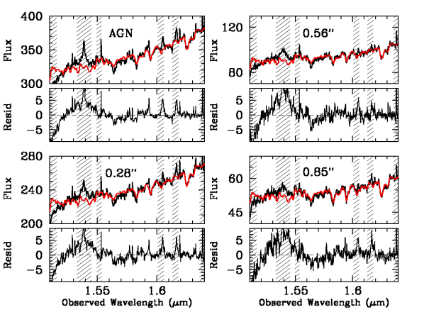
Figure 1.— Spectra from four spaxels of the rebinned NIFS datacube, with fluxes in arbitrary units (although the relative flux scaling between spaxels is correct). The best-fit spectra, obtained by convolving the LOSVDs from pPXF with the M0 template spectrum, are overplotted in light grey (colored red in the online version). The lower panel in each pair shows the residuals from each fit, in percentage units. The cross-hatched wavelength regions were excluded from the pPXF fitting in order to avoid contaminating spectral features (primarily AGN emission lines). The four pairs of panels are: (upper left) the central spaxel, where the AGN provides the majority of the flux; (lower left) a spaxel 0$\farcs$28 from the BH; (upper right) a spaxel 0$\farcs$56 from the BH; (lower right) a spaxel 0$\farcs$85 from the BH.

Figure 2 (top row) shows maps of the line-of-sight velocity ($V_{\rm los}$), velocity dispersion ($\sigma_{\rm los}$), and the 3rd and 4th GH moments ($h_{3},h_{4}$) in 0$\farcs$2 spaxels. The $x,y$ coordinates are aligned with the major and minor kinematic axes, respectively. The color scale is in km/s for $V_{\rm los}$ and $\sigma_{\rm los}$, and in dimensionless units for $h_{3}$ and $h_{4}$.

We then bi-symmetrize the 2D LOSVD map (Fig. 2 bottom row) around the kinematic minor axis at a position angle of $-65^{\circ}$ ($-50^{\circ}$ relative to the NIFS y-axis), using an IDL routine developed by van den Bosch & de Zeeuw (2010). This procedure enhances the S/N by combining the measurements on either side of the kinematic minor axis in a symmetric ($\sigma_{\rm los}$ and $h_{4}$), or anti-symmetric ($V_{\rm los}$ and $h_{3}$) way. Such a procedure is necessary in order to obtain sensible results from an axisymmetric dynamical modeling code, which assumes such an underlying symmetry. The kinematic data were bi-symmetrized in a weighted mean, using the individual uncertainties reported by pPXF to derive the weights. The final kinematic uncertainties are computed as the errors in the weighted mean values.

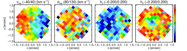
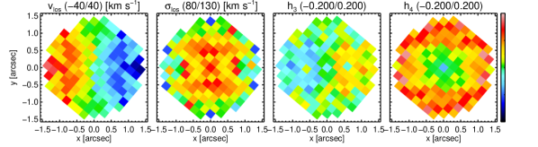
Figure 2.— Maps of line-of-sight velocity ($V_{\rm los}$), velocity dispersion ($\sigma_{\rm los}$) and the 3rd and 4th Gauss-Hermite (GH) moments ($h_{3},h_{4}$) in 0$\farcs$2 spaxels. The $x,y$ coordinates are aligned with the major and minor kinematic axes, respectively. The minimum and the maximum values of the color scale are indicated in the title of each panel in parenthesis ($V_{\rm los},\sigma_{\rm los}$ in km/s; $h_{3},h_{4}$ in dimensionless units). The top row shows the original kinematical data while the bottom row shows the kinematics after it is bi-symmetrized.

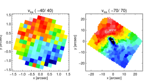
Figure 3.— Comparison of stellar velocity fields observed with the NIFS IFU (left) and SAURON IFU (right; Dumas et al. 2007). The AO-assisted NIFS data are consistent with the larger scale velocity map, but probe a spatial region inaccessible to the optical data because the AGN emission precludes measurements of the central stellar dynamics (the black region in the right panel). In both figures North is up and East is left.

Figure 3 shows the line-of-sight stellar velocity fields from NIFS (left) and SAURON (right). The latter data are from Dumas et al. (2007) and show a similar large scale rotational velocity to that seen in the inner 3″$\times$3″ region observed with NIFS. Although the large scale line-of-sight velocity fields in both panels show the same global rotational velocity, the central region of the SAURON velocity field within  5″$\times$ 5″ (right) is dominated by AGN continuum. Therefore, the innermost parts allow no velocity measurement, and appear as a black oval region in the image. Thus, the SAURON data do not provide constraints on the BH mass, although they could provide constraints on the mass-to-light ratio ($\Upsilon$). However, we do not include the SAURON data in our modeling, relying instead on the long-slit kinematics obtained from MMT and KPNO to provide the constraints on $\Upsilon$ at large radii. This is partly a pragmatic choice since the use of IFU data on both small and large scales would significantly increase the total number of kinematic constraints that would need to be fitted and, therefore, would require a significantly larger orbit library than we use here, making the problem significantly more computationally expensive than we are able to handle.

3.2. Surface Brightness Profile

We calculate the $H$-band surface brightness profile using our nested series of images to probe different spatial scales. For large radii ($5\arcsec-90\arcsec$), we use the photometrically calibrated OSUBSGS images. At intermediate radii ($1\arcsec-11\farcs 25$), we use the ACS optical image, allowing a significant region of overlap with the OSUBSGS data. The ACS flux level is then rescaled to provide the best match to the $H$-band data in the overlap region. Our use of the optical data could potentially bias the surface brightness profile we derive if there are significant variations in extinction or stellar population at radii of $1\arcsec-5\arcsec$. However, there are no independent indications of stellar population changes in that part of NGC 4151, and the radial profile of the ACS image is relatively smooth at those distances. Those radii are also well isolated from the PSF of the AGN in the ACS image.

In the central regions, we derive a stellar flux profile directly from the NIFS datacube. One of the outputs of the pPXF modeling is the derived amplitude of the stellar template that best matches the galaxy data. As our template spectra are continuum-normalized, these amplitudes constitute relative measurements of the stellar flux in each spaxel, calculated in a way that naturally omits the AGN contribution to the light profile. The unbinned data are used to probe radii of 0$\farcs 04-1\farcs 2$ (excluding the AGN-dominated central spaxel). The overall NIFS stellar profile is then scaled in amplitude to match the overlapping ACS data from larger radii.

We then fit the full $H$-band surface brightness profile using the Multi-Gaussian Expansion (MGE) package (Emsellem et al., 1994; Cappellari, 2002). The MGE routine fits the smallest necessary number of nested 2D Gaussians with a common center and radially varies their amplitudes and axis ratios to obtain the best possible smooth fit to the observed 2D surface brightness distribution, taking account of the PSF. The deprojection of a 2D surface brightness distribution to derive the 3D luminosity distribution suffers from the well known degeneracy arising from “konus densities” that are invisible in projection (Gerhard & Binney, 1996; Kochanek & Rybicki, 1996). A number of different methods have been used to derive the 3D luminosity density, none of which guarantee a unique deprojection. The MGE method has the advantage that, once an angle of inclination is assumed, each 2D Gaussian has a unique 3D luminosity density whose potential is easily computed and which is positive everywhere (Cappellari, 2002). The code outputs the amplitude (total counts), width in pixels ($\sigma_{pix}$), and observed axis ratio ($q$) for each Gaussian. We convert those values to a central surface brightness, $I_{H}$, for each Gaussian as:

$$\log_{10}I_{H}{\rm(L_{\odot,H}/pc^{2})}=0.4(\mu_{\odot,H}-\mu_{H}),$$ (1)

where $\mu_{\odot,H}$ is the $H$-band surface brightness of the Sun at a distance where 1 pc² subtends 1 arcsec². For an absolute $H$-band magnitude of 3.32$\pm$0.03 mag (Binney & Merrifield, 1998), this gives $\mu_{\odot,H}=22.89$ mag arcsec^-2. The surface brightness is computed from the MGE fits as:

$$\mu_{H}=m_{0}-2.5\log_{10}(\frac{C_{tot}}{2\pi q\sigma_{pix}^{2}})+5\log_{10}S_{pix}-A_{H},$$ (2)

where $m_{0}$ is the OSUBSGS $H$-band image zero-point of 22.2 mag, $C_{tot}$ is the total counts, $S_{pix}$ is the plate scale of $1\farcs 5$ pixel^-1, and the $H$-band extinction is $A_{H}$=0.016 mag (Schlegel et al., 1998, retrieved from the NASA/IPAC Extragalactic Database). For the MGE modelling, a 1-component PSF was used, having an effective width of $\sigma=0.05$.

The output of our MGE fit to the surface brightness distribution is given in Table 1. For each Gaussian in the MGE fit, the first column gives an identifying number, the second column gives the $H$-band luminosity density, the third column gives the standard deviation $\sigma$ (in arcsec), and the fourth column gives the flattening $q$ (ellipticity). It is clear from the values of $q$ in the third column that the bulge surface brightness distribution is close to circular since most of the Gaussians have $q\sim 1$ (except for the innermost and outermost Gaussians) suggesting that the bulge is probably close to spherical. In Figure 4, we show the composite radial surface brightness profile obtained by patching together the three imaging datasets.

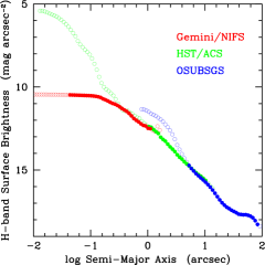
Figure 4.— Composite $H$-band radial surface brightness profile of the bulge, consisting of data from Gemini/NIFS at small radii (colored red in the online version), HST/ACS at intermediate radii (colored green in the online version), and OSUBSGS at large radii (colored blue in the online version). The OSUBSGS and HST/ACS surface brightness profiles both turn upwards at small radii because of the AGN. The NIFS profile comes from the amplitude of the stellar features in each spaxel and so naturally omits the AGN. The open points, which are contaminated by AGN flux, are not used in the MGE fit to the SB profile. In contrast to the data in Table 1, the values plotted here have not been corrected for the PSF, in order to more clearly show the radial regions free from AGN contamination.

Table 1MGE Fit to Surface brightness distribution

Gaussian	Surface Density, $I_{H}$	Gaussian $\sigma$	Axis Ratio $q$
Number	($L_{\odot,H}$/pc2)	(″)
(1)	(2)	(3)	(4)
1	9.3963E+04	0.126	0.7906
2	1.3200E+05	0.232	1.0000
3	7.8100E+04	0.549	1.0000
4	2.0951E+04	1.421	1.0000
5	6.7191E+03	2.799	1.0000
6	3.7009E+03	6.703	1.0000
7	6.8485E+02	14.513	0.9550
8	3.1906E+02	64.987	0.7052

3.3. Mass-to-Light Ratio

To provide a rough constraint on the relationship between the luminosity distribution and the stellar mass distribution, we combine optical imaging from SDSS with the OSUBSGS $H$-band image. We construct ($g-i$) and ($i-H$) color maps of NGC 4151, finding the bulge colors of ($g-i$)=1.1$\pm$0.1 mag, and ($i-H$)=2.4$\pm$0.2 mag to be quite uniform across the bulge (aside from the central few arcseconds, where the AGN dominates the emission). Zibetti et al. (2009) calculated $H$-band mass-to-light ratios ($\Upsilon_{H}$) in ($g-i$)-($i-H$) color-space, based on a Monte Carlo analysis of Bruzual & Charlot (2003) stellar population synthesis models. Examining our measured colors in the Zibetti et al. (2009) color-space indicates that $\Upsilon_{H}=0.4\pm 0.2~{}{{\mathrm{M}}_{\odot}}/{{\mathrm{L}}_{\odot}}$. Our initial exploration with dynamical models spanning the entire range $0.2~{}{{\mathrm{M}}_{\odot}}/{{\mathrm{L}}_{\odot}}<\Upsilon_{H}<0.6~{}{{\mathrm{M}}_{\odot}}/{{\mathrm{L}}_{\odot}}$ showed that the best fit values were always in the range $0.2~{}{{\mathrm{M}}_{\odot}}/{{\mathrm{L}}_{\odot}}<\Upsilon_{H}<0.425~{}{{\mathrm{M}}_{\odot}}/{{\mathrm{L}}_{\odot}}$, hence this range of values is used in the models below.

3.4. Morphological Classification

NGC 4151 was classified by de Vaucouleurs et al. (1991) as (R’)SAB(rs)ab: a disk galaxy with a pseudo-outer ring (R’), a “mixed” bar (AB) (i.e., possibly barred but is not strongly so), with mixed spiral/inner ring classification (rs), and an intermediate to large bulge (ab). Figure 5 (left) shows the Palomar Observatory Sky Survey (POSS) image of NGC 4151 in the red optical filter. In part because of the very circular bulge, the classification of this galaxy as barred has been questioned by authors as far back as Davies (1973), who speculated that the elongation was not a bar, but was in fact made up of material that was ejected from the nucleus in a former explosive event. However, we believe that NGC 4151 may be an example of a galaxy containing a “barlens”, an oval-shaped structure that is likely to be the vertically thick aspect of a bar seen from a particular viewing angle (Laurikainen et al., 2011; Athanassoula et al., 2014).

In Paper I, we assumed that the kinematic major axis is aligned with the bar, since spectral information was only available along two long-slits. The KPNO slit (represented by the red line in Fig. 5 left) was oriented along the bar at a position angle of 135^∘ (Ferrarese et al., 2001). The MMT slit (green line in Fig. 5 left) was placed at a position angle of 69^∘. The middle panel of Figure 5 shows the region within the white box from the left panel. The grey box in the middle panel represents the orientation and shape of the NIFS field of view. It is quite clear from a comparison of the NIFS velocity field and the SAURON velocity field in Fig. 3, that the rotation axis of the disk and bulge are not perpendicular to the bar as was assumed in Paper I. This is an important difference between the models presented here and the models presented in Paper I.

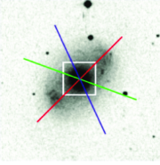
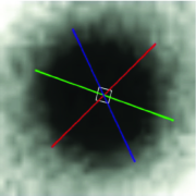
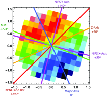
Figure 5.— Orientation of long-slits and NIFS field to kinematic and photometric axes of the galaxy. Left: Optical image of NGC 4151 (from POSS). North is at top, East at left. The field-of-view is 5′$\times$5′. The white box is 1′$\times$1′and is shown zoomed-in in the middle panel. The red line shows the orientation of the KPNO slit (2″wide), the green line shows the orientation of the MMT slit (1″wide), the blue line shows the orientation of the major axis of the bulge as inferred from the symmetry axis of the velocity field (see right panel). Middle: the nuclear region 1′$\times$1′; the grey box shows the size and orientation of the NIFS field. Right: Symmetrized NIFS velocity field showing inferred kinematic major axis (blue line), minor axis (Z; ochre line). The angles of the slits and NIFS instrument are given relative to the kinematic major axis.

3.5. Distance to NGC 4151

To first order, the BH mass derived by the stellar dynamical modeling depends linearly on the assumed distance to the galaxy. For consistency with the analysis in Paper I, we adopt a distance for NGC 4151 of 13.9 Mpc (based on the recession velocity of 998 ${\mathrm{km\,s^{-1}}}$ measured by Pedlar et al., 1992). However, as noted in Paper I, the actual distance to the galaxy is rather uncertain, with published estimates spanning a range of 10 Mpc to 30 Mpc. Recently, Tully et al. (2009) compiled a group-averaged Tully-Fisher distance of 11.2$\pm$1.1 Mpc in the Extragalactic Distance Database. However, that group distance is based on just four galaxies, which have a standard deviation in their distance moduli of more than four times the individual distance modulus errors. Furthermore, it is unclear whether the contribution to the group average distance from NGC 4151 (of $\sim$4 Mpc) accounts for the AGN contribution to the galaxy brightness. Thus, we cannot regard the Tully et al. (2009) value as being any more reliable than other distances, and until a more accurate distance can be obtained, we continue to use the value of 13.9 Mpc.

4. Stellar Dynamical Modeling

We apply what is now the standard stellar dynamical modeling approach of orbit superposition (e.g Schwarzschild, 1979; van der Marel et al., 1998; Cretton et al., 1999; Gebhardt et al., 2003; Valluri et al., 2004) to fit the observed LOSVDs and luminosity distribution of NGC 4151. The orbit superposition (or “Schwarzschild”) method of dynamical modeling uses line-of-sight kinematical and imaging data to constrain the mass distributions of external galaxies. The implementation of the code used here differs from the method detailed in Valluri et al. (2004, hereafter VME04) in two small aspects. It is (a) designed to fit generalized axisymmetric models that are obtained from direct deprojection of the surface brightness profiles of the individual galaxies using a MGE code, following the method outlined in Cappellari (2002); (b) modified to fit integral field kinematics in addition to long-slit kinematics.

4.1. Model Setup

We restrict our models to the surface brightness distribution within 50″— i.e., the bulge region — using the MGE decomposition from Table 1. For each dynamical model, we assume a constant $H$-band mass-to-light ratio ($\Upsilon_{H}$) for the stars, with values varying from $0.2~{}{{\mathrm{M}}_{\odot}}/{{\mathrm{L}}_{\odot}}-0.425~{}{{\mathrm{M}}_{\odot}}/{{\mathrm{L}}_{\odot}}$. The resulting density profile is then converted to a gravitational potential using an axisymmetric multipole expansion scheme (Binney & Tremaine, 2008). The gravitational potential of a point mass (${{\mathrm{M}}_{\rm BH}\,}$), representing the central BH, is then added. Models are constructed for every pair of parameters (${{\mathrm{M}}_{\rm BH}\,}$, $\Upsilon_{H}$), building an orbit library for each combination.

The large-scale H I disk of NGC 4151 is inclined to the line of sight at $i=20^{\circ}-25^{\circ}$ (Simkin, 1975). However, since the bulge appears very close to circular in projection (see Fig. 5 and Tab. 1), it is probably nearly spherical or being viewed close to face on. Thus, we run models on a 2D grid of (${{\mathrm{M}}_{\rm BH}\,},\Upsilon_{H}$) values for three different inclination angles $i=90^{\circ}$ (edge-on), $i=60^{\circ}$ and $i=23^{\circ}$ (close to face-on). We also run a limited set of models for which the value of ${{\mathrm{M}}_{\rm BH}\,}$ is held fixed while the inclination angle of the model is varied with values $i=15^{\circ},30^{\circ},50^{\circ}$, and $75^{\circ}$, in an effort to set constraints on the inclination of the bulge to the line-of-sight.

For inclination angles of $i=90^{\circ}$ and $23^{\circ}$, we run orbit libraries for 18 BH masses between $1\times 10^{4}~{}{{\mathrm{M}}_{\odot}}-2.6\times 10^{8}~{}{{\mathrm{M}}_{\odot}}$, using a baseline $\Upsilon_{H}=0.3~{}{{\mathrm{M}}_{\odot}}/{{\mathrm{L}}_{\odot}}$. These models are then scaled to create libraries for 18 different $\Upsilon_{H}$ values, producing a total of 324 models for each inclination angle. We also run orbit libraries for $i=60^{\circ}$, using 10 BH masses across the same mass range and 18 $\Upsilon_{H}$ values for each ${{\mathrm{M}}_{\rm BH}\,}$ (180 models). The range of BH mass values was set by initial experimentation with a coarse grid on a wide range of values. The lowest two values of ${{\mathrm{M}}_{\rm BH}\,}$ are set to 10${}^{4}~{}{{\mathrm{M}}_{\odot}}$ and 10${}^{7}~{}{{\mathrm{M}}_{\odot}}$, both of which consistently give poor fits to the data. The upper limit of ${{\mathrm{M}}_{\rm BH}\,}$ was raised until it was clear that models once again gave very poor fits to the data.

The combined gravitational potential of the bulge and the BH is used to integrate a large library of $N_{o}$ stellar orbits selected on a grid with $N_{E}$ energy values, $N_{A}$ angular momentum values ($L_{z}$) at each energy, and $N_{I3}$ pseudo third integral values ($I_{3}$) at each angular momentum value (see VME04 for details). For instance, models with $N_{o}=9936$ used $N_{E}=46$, $N_{A}=24$, $N_{I3}=9$. Each orbit is integrated for 100 orbital periods and its average “observed” contribution to each of the “apertures” in which kinematical data are available is stored. The orbital kinematics are subjected to the same type of instrumental effects as the real data (i.e. PSF convolution, pixel binning).

Self-consistent orbit-superposition models are constructed by linearly co-adding orbits in each library to simultaneously fit several elements within the observed apertures (imaging and spectroscopic): the 3D mass distribution (for each value of $\Upsilon_{H}$), the projected surface density distribution, and the LOSVDs. The fits use a non-negative least squares optimization algorithm (NNLS; Lawson & Hanson, 1974), which gives the weighted superposition of the orbits that best reproduce both the self-consistency constraints (i.e., the 3D mass distribution and surface brightness distribution) and the observed kinematical constraints ($V_{\rm los},\sigma_{\rm los},h_{3},h_{4}$).

VME04 showed that as the ratio of orbits to constraints decreases, the error bars decrease artificially. In the majority of the models presented here we have 1240 constraints that are fitted by a library of 9936 orbits. This size of orbit library gives an orbits-to-constraints ratio of 8 which is only slightly above the ratio (5) at which VME04 find that solutions begin to be biased. In Section 5.3.1 we carry out a limited exploration with a 50% larger orbit library and find that our results are unchanged.

Smoothing (or “regularization”) of the orbital solutions is typically performed in this type of analysis, and a variety of methods have been employed to that end. Regularization mainly helps to reduce the sensitivity of the solutions to noise in the data by requiring a smoother sampling of the orbit libraries used in the solution. Following Cretton et al. (1999), we run a trial series of models with a regularization scheme that requires local smoothing in phase space. We find that for small smoothing parameters ($\lambda=0.1$) the resultant best-fit ${{\mathrm{M}}_{\rm BH}\,}$ values do not differ from the models without regularization. However, the $\chi^{2}$ value for the best-fit model is larger and the error bars on ${{\mathrm{M}}_{\rm BH}\,}$ are smaller. VME04 showed that it is impossible (without computationally expensive approaches such as generalized cross-validation) to determine the ideal regularization parameter. Not regularizing the solutions can yield large error bars, but choosing too large a value of the smoothing parameter can introduce a bias in the best-fit value of ${{\mathrm{M}}_{\rm BH}\,}$. In this paper, we present models without regularization, since imposing regularization constraints significantly increases the total number of constraints and therefore decreases even further the orbits-to-constraints ratio. For the libraries used here, models without regularization provide the most conservative error bars on the estimated value of ${{\mathrm{M}}_{\rm BH}\,}$.

Figure 6.— Contours of constant fractional error in enclosed mass and aperture surface brightness (self-consistency constraints) in the plane of parameters $\Upsilon_{H}$ and ${{\mathrm{M}}_{\rm BH}\,}$ for models with inclination to the line of sight $i=90^{\circ}$. The star marks the location of the model with 0.27% fractional error per constraint. Contours are spaced at intervals of 0.1% fractional error per constraint.

4.2. Model Self-Consistency Constraints

Since the mass and surface mass density constraints are self-consistency constraints rather than observational constraints, they do not have observational errors associated with them. There are two ways in which the absence of observational errors are handled in the literature. Cretton et al. (1999) and VME04 include self-consistency constraints in the NNLS minimization problem with errors corresponding to predefined level of relative accuracy in the fit (e.g. 5% -10%), while others (Gebhardt et al., 2003; van den Bosch et al., 2008) solve the orbit superposition problem by requiring the self-consistency constraints (mass and surface brightness) to be fitted as separate as linear (in)equality constraints with predetermined absolute accuracy. van den Bosch et al. (2008) state that they require the self-consistency constraints to be fitted to an accuracy of 0.02. We also attempted to fit self-consistency constraints as linear equalities but find that that since the values of the mass constraints vary by 5 orders of magnitude (from $10^{-4}$ to 10), using a fixed numerical accuracy fails to fit the mass constraints at small radii (where the logarithmic radial bins have the smallest mass values per bin and where the fit to mass constraints most strongly affects the estimated ${{\mathrm{M}}_{\rm BH}\,}$).

For the models presented here we include the self-consistency constraints in the optimization problem and require the optimization problem to fit each of the 472 self-consistency constraints (280 mass constraints and 192 aperture surface brightness constraints) with an error corresponding to a relative accuracy-per-constraint of 5%. For our preferred model with $i=90^{\circ}$, the fractional accuracy per self-consistency constraint varies from 0.27% (for the best fit model) to 2.2% for the worst fit model, i.e., always better than our required accuracy. Figure 6 shows contours of constant fractional error in the fit to the self-consistency constraints (mass and surface brightness in apertures) over the 2D parameter space (${{\mathrm{M}}_{\rm BH}\,}$, $\Upsilon_{H}$) for models with $i=90^{\circ}$. The star is the location of the model with 0.27% accuracy per self-consistency constraint, and the contours are spaced at intervals of 0.1% relative accuracy per constraint.

In previous applications of our Schwarzschild modeling code (VME04, Valluri et al., 2005, Paper I), the error in the fit to the self-consistency constraints was essentially random over the entire 2D parameter space (${{\mathrm{M}}_{\rm BH}\,},\Upsilon$). Although the self-consistency constraints were always included in the $\chi^{2}$, they contributed so little to the total $\chi^{2}$ that the best fit solution was always driven by the fit to the kinematical constraints. We will show that this is not true for our current NGC 4151 dataset. Despite the fact that the fits to the 3D mass distribution and surface brightness distribution are very good, because the fit vary systematically rather than randomly across the parameter space, the best fit solution is altered by the decision of whether or not to include the fit to the self-consistency constraints in the $\chi^{2}$.

Based on the arguments above, we compute the $\chi^{2}$ in two different ways: (1) the total ${{\chi^{2}}_{\rm all}}$ includes all the constraints in the NNLS optimization problem: 280 mass constraints, 192 surface brightness constraints, and 768 kinematical constraints (giving a total of $N_{c}=1240$ constraints); (2) ${{\chi^{2}}_{\rm kin}}$ which only considers the quality of the fit to $N_{c}=768$ kinematical constraints ($V_{\rm los},\sigma_{\rm los},h_{3},$ and $h_{4}$ in 192 apertures: 136 NIFS spaxels, 15 KPNO apertures, and 41 MMT apertures). For each of the three assumed angles of inclination for the bulge, we construct models by fitting these constraints using an orbit library consisting of $N_{o}=9936$ orbits. For one inclination angle ($i=90^{\circ}$) we do a limited exploration with a library consisting of $N_{o}=15092$ orbits. After generating orbit libraries for a grid of parameters (${{\mathrm{M}}_{\rm BH}\,},\Upsilon_{H}$) the best fit parameters are determined by the minimum in the 2D $\chi^{2}$-contour plot.

5. Results

In this section, we present the results of our modeling. In Section 5.1 we describe results for inclination angles $i=90^{\circ}$, $i=60^{\circ}$ and $i=23^{\circ}$, showing 2D contour plots of ${{\chi^{2}}_{\rm all}}$ and ${{\chi^{2}}_{\rm kin}}$ using a full 2D grid of models for each of these inclination angles. In Section 5.2 we examine the dependence on inclination angle for 4 additional models using a single ${{\mathrm{M}}_{\rm BH}\,}$. In Section 5.3 we explore the robustness of our solutions by examining their sensitivity to the size of the orbit library and to the effect of restricting the set of kinematic constraints to those from the nuclear region only. We also present some of the best-fit solutions and show how well different pairs of ${{\mathrm{M}}_{\rm BH}\,},\Upsilon_{H}$ fit both the 1D and 2D kinematical data. In Section 5.4, we discuss our results in the context of the M${}_{\rm BH}-\sigma$ relation.

5.1. Dependence on Definition of $\chi^{2}$

Figure 7 shows 2D contour plots of ${{\chi^{2}}_{\rm all}}$ in the plane of model parameters ${{\mathrm{M}}_{\rm BH}\,}$ and $\Upsilon_{H}$ for $i=90^{\circ}$ (top), $i=60^{\circ}$ (middle), and $i=23^{\circ}$ (bottom). The grid of points shows the model parameters (${{\mathrm{M}}_{\rm BH}\,},\Upsilon_{H}$) for which the orbit libraries is constructed and the optimization problem is solved. The first 6 contour levels in all the $\chi^{2}$ contour plots that follow correspond to $\Delta\chi^{2}=2.3~{}(1\sigma$, 68.3% confidence), $\Delta\chi^{2}=4.61~{}(2\sigma$, 90% confidence), $\Delta\chi^{2}=6.17~{}(3\sigma$, 95.4% confidence), $\Delta\chi^{2}=9.21~{}(4\sigma$, 99% confidence), $\Delta\chi^{2}=11.9~{}(5\sigma$, 99.73%), and $\Delta\chi^{2}=18.4~{}(6\sigma$, 99.99%), with subsequent contours equally spaced in $\Delta\chi^{2}$.

Figure 7.— Contours of constant ${{\chi^{2}}_{\rm all}}$ in the plane of model parameters $\Upsilon_{H}$ and ${{\mathrm{M}}_{\rm BH}\,}$ for models (each with $N_{o}=9936$) with inclination to the line of sight $i=90^{\circ}$ (top), $i=60^{\circ}$ (middle), and $i=23^{\circ}$ (bottom). The star in each plot marks the location of the best-fit values for M_BH and $\Upsilon_{H}$ (see Tab. 2 for details). The first six contours surrounding the star are the $1\sigma,2\sigma,\ldots,6\sigma$ confidence intervals respectively. Subsequent contours are equally spaced between the 6th contour and the maximum $\chi^{2}$ value.

For $i=90^{\circ}$, the minimum value of ${{\chi^{2}}_{\rm all}}$ is obtained for ${{\mathrm{M}}_{\rm BH}\,}=4.68\times 10^{7}~{}{{\mathrm{M}}_{\odot}}$ and $\Upsilon_{H}=0.304~{}{{\mathrm{M}}_{\odot}}/{{\mathrm{L}}_{\odot}}$, with $({{\chi^{2}}_{\rm all}})_{\rm min}=709.1$. For inclination angle of $i=60^{\circ}$, the best fit model has ${{\mathrm{M}}_{\rm BH}\,}=5.42\times 10^{7}~{}{{\mathrm{M}}_{\odot}}$ and $\Upsilon_{H}=0.305~{}{{\mathrm{M}}_{\odot}}/{{\mathrm{L}}_{\odot}}$, with $({{\chi^{2}}_{\rm all}})_{\rm min}=767.5$. For inclination angle of $i=23^{\circ}$, the best fit model has ${{\mathrm{M}}_{\rm BH}\,}=3.69\times 10^{7}~{}{{\mathrm{M}}_{\odot}}$ and $\Upsilon_{H}=0.304~{}{{\mathrm{M}}_{\odot}}/{{\mathrm{L}}_{\odot}}$, with $({{\chi^{2}}_{\rm all}})_{\rm min}=1050.8$.

Figure 8.— $\Delta{{\chi^{2}}_{\rm all}}$ curves marginalized over $\Upsilon_{H}$ (top) and marginalized over ${{\mathrm{M}}_{\rm BH}\,}$ (bottom) in Fig. 7, for $i=90^{\circ}$ (solid), $i=60^{\circ}$ (dashed) $i=23^{\circ}$ (dot-dashed). The thin horizontal dotted lines corresponds to $\Delta{{\chi^{2}}_{\rm all}}=1$ (1$\sigma$, 68.5% confidence interval), $\Delta{{\chi^{2}}_{\rm all}}=2.71$ (2$\sigma$, 95%) and $\Delta{{\chi^{2}}_{\rm all}}=6.63$ (3$\sigma$, 99%).

Table 2 summarizes the results and includes minimum $\chi^{2}$ values and the 1$\sigma$ and 3$\sigma$ error bars. The errors on a given parameter are obtained by marginalizing the 2D $\chi^{2}_{\rm all}$ values over the other parameter. Figure 8 (top) shows the marginalized 1D $\Delta\chi^{2}$ versus ${{\mathrm{M}}_{\rm BH}\,}$ for the three different inclination angles, as indicated by the legends. The horizontal dotted lines are at $\Delta\chi^{2}=1$ (1$\sigma$, 68.5% confidence interval for 1 degree-of-freedom), $\Delta\chi^{2}=2.71$ (2$\sigma$, 90% confidence interval), and $\Delta\chi^{2}=6.63$ (3$\sigma$, 99% confidence interval). The 1$\sigma$ and 3$\sigma$ errors on ${{\mathrm{M}}_{\rm BH}\,}$ and $\Upsilon_{H}$ are given in Table 2. Likewise, Figure 8 (bottom) shows the marginalized 1D $\Delta\chi^{2}$ versus $\Upsilon_{H}$ for each of the three inclinations of models to the line-of-sight.

It is important to note that with the standard methods used to derive the velocity profiles (VPs) from the spectra, the errors in the Gauss-Hermite (GH) coefficients are not independent. The errors associated with the even moments ($\sigma$ and $h_{4}$) are correlated, and errors associated with the odd moments ($V$ and $h_{3}$) are also correlated (see, e.g., Joseph et al., 2001; Cappellari & Emsellem, 2004). Houghton et al. (2006) point out that an important consequence of correlated errors in the GH coefficients is that the errors obtained by comparing data to dynamical models using the $\chi^{2}$ estimator are significantly underestimated. In this paper we quote both 1-$\sigma$ and 3-$\sigma$ errors, and often consider the 3-$\sigma$ errors as better representations of the true modeling errors.

Table 2Best-fit values of ${{\mathrm{M}}_{\rm BH}\,}$ and $\Upsilon_{H}$ and error bars

$i$	$N_{o}$	$\chi^{2}_{\rm min}$	${{\mathrm{M}}_{\rm BH}\,}(10^{7}~{}{{\mathrm{M}}_{\odot}}$)			$\Upsilon_{H}$ (${{\mathrm{M}}_{\odot}}/{{\mathrm{L}}_{\odot}}$)
(∘)			best-fit	1$\sigma$	3$\sigma$	best-fit	1$\sigma$	3$\sigma$
(1)	(2)	(3)	(4)	(5)	(6)	(7)	(8)	(9)
$\chi^{2}_{\rm all}$ includes mass, surface brightness, kinematics, $N_{c}=1240$
90∘	9936	709.1	4.68	${}^{+0.46}_{-0.41}$	${}^{+1.10}_{-1.40}$	0.304	$\pm 0.002$	$\pm 0.005$
60∘	9936	767.5	5.42	${}^{+0.73}_{-0.78}$	${}^{+1.82}_{-2.2}$	0.305	$\pm 0.003$	$\pm 0.006$
23∘	9936	1050.8	3.69	${}^{+0.25}_{-0.16}$	${}^{+0.62}_{-0.47}$	0.304	$\pm 0.003$	$\pm 0.005$
$\chi^{2}_{\rm kin}$ includes only kinematics, $N_{c}=768$
90∘	9936	186.7	7.76	${}^{+1.92}_{-1.89}$	${}^{+4.20}_{-4.09}$	0.332	$\pm 0.008$	$\pm 0.022$
60∘	9936	193.1	8.62	${}^{+1.22}_{-1.26}$	${}^{+3.35}_{-3.10}$	0.326	$\pm 0.006$	$\pm 0.019$
23∘	9936	348.2	8.50	${}^{+1.01}_{-1.07}$	${}^{+3.69}_{-3.25}$	0.329	$\pm 0.004$	$\pm 0.013$

The best fit solutions for both ${{\mathrm{M}}_{\rm BH}\,}$ and $\Upsilon_{H}$ for the three different inclination angles are consistent with each other within 3$\sigma$. However $({{\chi^{2}}_{\rm all}})_{\rm min}$ is the smallest for the edge-on model ($i=90^{\circ}$), increases for $i=60^{\circ}$ and is significantly larger for $i=23^{\circ}$ implying that it may be possible to constrain the inclination of the bulge (see Section 5.2). Marginalizing ${{\chi^{2}}_{\rm all}}$ over the three values of inclination gives a best fit ${{\mathrm{M}}_{\rm BH}\,}\sim 5\times 10^{7}{{\mathrm{M}}_{\odot}}$ and $\Upsilon_{H}\sim 0.30{{\mathrm{M}}_{\odot}}/{{\mathrm{L}}_{\odot}}$.

Figure 9 shows 2D contour plots of $\chi_{\rm kin}$ for the same sets of models as in Figure 7, with inclination angles $i=90^{\circ},60^{\circ},23^{\circ}$ (from top to bottom). We emphasize that the model solutions that are used to generate Figure 9 are identical to those used to generate Figure 7 – only the quantities used in computing the $\chi^{2}$ of the fit to the data differ.

Figure 10 shows the same data marginalized over $\Upsilon_{H}$ (top) and marginalized over ${{\mathrm{M}}_{\rm BH}\,}$ (bottom). It is clear from these two figures that the best-fit solutions obtained using $\chi^{2}_{\rm kin}$ give both a larger ${{\mathrm{M}}_{\rm BH}\,}\sim 8\times 10^{7}~{}{{\mathrm{M}}_{\odot}}$ and a larger $\Upsilon_{H}\sim 0.33~{}{{\mathrm{M}}_{\odot}}/{{\mathrm{L}}_{\odot}}$. We will discuss the possible causes for this in Section 5.3 and Section 6.

Figure 9.— Contours of constant $\chi^{2}_{\rm kin}$, where $\chi^{2}$ is computed only from the fit to the kinematic constraints for models with inclination to the line of sight $i=90^{\circ}$. The stars mark the location of the best-fit values for M_BH and $\Upsilon_{H}$. The first 6 contour levels in all three plots correspond to $1\sigma,2\sigma,\ldots,6\sigma$ confidence intervals respectively, with subsequent contours being equally spaced.

Figure 10.— Similar to Fig. 8, $\Delta\chi^{2}_{\rm kin}$ curves marginalized over $\Upsilon_{H}$ (top) and marginalized over ${{\mathrm{M}}_{\rm BH}\,}$ (bottom) in Fig. 9.

5.2. Dependence on Inclination Angle of Bulge

In contrast to the results of Paper I, where $i=90^{\circ}$ models gave an upper limit of ${{\mathrm{M}}_{\rm BH}\,}<4\times 10^{7}{{\mathrm{M}}_{\odot}}$ and $i=23^{\circ}$ models gave a best fit ${{\mathrm{M}}_{\rm BH}\,}$ between $4-5\times 10^{7}{{\mathrm{M}}_{\odot}}$, Figures 8 and 10 show that best-fit ${{\mathrm{M}}_{\rm BH}\,}$ is relatively insensitive to inclination (although the actual best-fit value depends on how $\chi^{2}$ was computed). Table 2 shows that the minimum values of $\chi^{2}_{\rm all}$ and $\chi_{\rm kin}^{2}$ for $i=90^{\circ}$ are lower than the corresponding $\chi^{2}$ values for the other two inclination angles. We now try to constrain the inclination angle of the bulge of NGC 4151 by assuming a constant BH mass of ${{\mathrm{M}}_{\rm BH}\,}=5\times 10^{7}~{}{{\mathrm{M}}_{\odot}}$. With this value of ${{\mathrm{M}}_{\rm BH}\,}$ we compute orbit libraries for four additional inclination angles: $15^{\circ}$, $30^{\circ}$, $50^{\circ}$, and $75^{\circ}$. Figure 11 shows the values of $\chi^{2}_{\rm all}$ for models with this value of ${{\mathrm{M}}_{\rm BH}\,}$ and $\Upsilon_{H}=0.31~{}{{\mathrm{M}}_{\odot}}/{{\mathrm{L}}_{\odot}}$ as a function of the inclination of the bulge to the line-of-sight. It is clear that $\chi^{2}_{\rm all}$ decreases steadily with increasing inclination angle with a minimum at $i=90^{\circ}$. (A similar dependence on inclination angle is obtained for ${{\mathrm{M}}_{\rm BH}\,}=10^{8}~{}{{\mathrm{M}}_{\odot}}$, although all the models give much worse fits as assessed by the ${{\chi^{2}}_{\rm all}}$ values.)

The inclination angle of $i=23^{\circ}$ that is inferred from the H I velocity field is strongly disfavored. Since the disk of this galaxy is clearly seen to be close to face-on, the edge-on orientation of the bulge preferred by our models is rather puzzling: the surface brightness isophotes of the bulge are nearly circular, hence the best-fit edge-on orientation implies that the bulge is nearly spherical in shape; but in this case the rotation axis of the bulge must be misaligned with the rotation axis of the disk by $\sim 70^{\circ}$.

Previous determinations of the orientations of the various components of NGC 4151 have shown a remarkable diversity. While the circular H I isophotes of the large-scale disk suggest the nearly face-on orientation with $i=23^{\circ}$ (Simkin, 1975) – which motivated our testing of that value of inclination – the components associated with the AGN have been inferred to lie further from our line of sight. Models of the bi-conical narrow-line region (NLR) in the UV and optical (Das et al., 2005; Shimono et al., 2010; Crenshaw et al., 2010), and in the near-IR (Ruiz et al., 2003; Storchi-Bergmann et al., 2010; Müller-Sánchez et al., 2011) have typically found inclinations of $40^{\circ}-50^{\circ}$. Closer to the AGN, Gallimore et al. (1999) fit the H I absorption using a pc-scale nuclear disk inclined at $i=50^{\circ}$. On even smaller scales, an inclination of $20^{\circ}$ for the AGN accretion disk was obtained from modeling the X-ray spectrum (Takahashi et al., 2002), while Storchi-Bergmann et al. (2010) suggest that the radio jet in NGC 4151 lies very close to the plane of the sky and is interacting directly with circumnuclear gas in the plane of the galaxy (i.e., $i>60^{\circ}$). This lack of alignment between the different spatial scales could be the consequence of a merger in the galaxy’s recent past. It has been claimed that the periodic variability in the nuclear activity of NGC 4151 is indicative of a BH binary, with a separation on the order of $10^{3}$ AU (Bon et al., 2012). While distinguishing between a single BH and a close binary is far beyond the capability of our dataset, the remnants of a merger could also contribute to the complicated dynamics we observe on the size scales of the bulge. In Section 5.3, we will show that the kinematics in the inner 5″ show evidence for a bar in this region, implying that the internal dynamics of the bulge are likely not that of a spherical or axisymmetric system. A full understanding of why the kinematics of our model prefers an edge-on configuration to the more inclined configuration requires the system to be modeled by a bar dynamical modeling code, which does not exist at the present time.

Figure 11.— $\chi^{2}_{\rm all}$ as a function of model inclination for models with ${{\mathrm{M}}_{\rm BH}\,}=5.2\times 10^{7}~{}{{\mathrm{M}}_{\odot}}$ and $\Upsilon_{H}=0.31~{}{{\mathrm{M}}_{\odot}}/{{\mathrm{L}}_{\odot}}$. The edge-on model ($i=90^{\circ}$) gives the smallest $\chi^{2}_{\rm all}$.

Since the result of this section show that models with edge-on inclination ($i=90^{\circ}$) are greatly preferred over more face-on models, in the rest of this paper we confine our analysis to models with $i=90^{\circ}$.

5.3. Tests of Robustness and Kinematic Fits

Table 3Results of Robustness Tests

$\chi^{2}$ type	$N_{o}$	$N_{c}$	$\chi^{2}_{\rm min}$	$\chi^{2}_{\rm red}$	${{\mathrm{M}}_{\rm BH}\,}(10^{7}~{}{{\mathrm{M}}_{\odot}}$)			$\Upsilon_{H}$ (${{\mathrm{M}}_{\odot}}/{{\mathrm{L}}_{\odot}}$)
					best-fit	1$\sigma$	3$\sigma$	best-fit	$1\sigma$	$3\sigma$
(1)	(2)	(3)	(4)	(5)	(6)	(7)	(8)	(9)	(10)	(11)
$\chi^{2}_{\rm all}$	15092	1240	641.9	0.52	4.68	${}^{1.09}_{-0.99}$	${}^{+2.61}_{-2.23}$	0.31	$\pm 0.003$	$\pm 0.01$
$\chi^{2}_{\rm kin}$	15092	768	170.2	0.22	7.32	${}^{+1.18}_{-1.05}$	${}^{+3.82}_{-2.65}$	0.31	$\pm 0.01$	$\pm 0.03$
Fit includes NIFS data only
$\chi^{2}_{\rm all}$	9936	960	583.1	0.61	3.82	${}^{+1.00}_{-1.11}$	${}^{+1.55}_{-2.02}$	0.32	$\pm 0.01$	$\pm 0.02$
$\chi^{2}_{\rm kin}$	9936	680	101.7	0.14	3.70	${}^{+1.25}_{-1.26}$	${}^{+3.30}_{-2.0}$	0.35	$\pm 0.01$	$\pm 0.03$

VME04 showed that the solution derived from the Schwarzschild method was sensitive to two important factors: (a) the size of the orbit libraries used in obtaining the best-fit BH mass; and (b) the spatial resolution of the kinematic data and whether or not they resolved the sphere-of-influence of the BH. They showed that biased solutions could result when the size of the orbit libraries was too small for the available data. They also showed that when the kinematic data did not resolve the sphere-of-influence of the BH, spurious results could arise. In the next two sections we perform two tests to assess the robustness of our solutions. In particular, our goal is to assess which of the two values of ${{\mathrm{M}}_{\rm BH}\,}$ obtained previously (5$\times 10^{7}~{}{{\mathrm{M}}_{\odot}}$ or 8$\times 10^{7}~{}{{\mathrm{M}}_{\odot}}$) is more robust.

5.3.1 Dependence on Orbit Library Size

In this section, we construct a set of 288 models with $i=90^{\circ}$ but with orbit libraries containing $N_{o}=15092$ orbits (as compared to $N_{o}=9936$ used thus far) to fit the same set of 1240 constraints that were fitted in Section 5.1. Large orbit libraries are constructed for 16 BH masses between 10${}^{4}~{}{{\mathrm{M}}_{\odot}}$ and 15$\times 10^{7}~{}{{\mathrm{M}}_{\odot}}$ and for 18 values of $\Upsilon_{H}$.

Figure 12 shows the 1D $\chi^{2}_{\rm all}$ (solid curves) and $\chi^{2}_{\rm kin}$ (dashed curves) obtained by marginalizing over the mass-to-light ratio $\Upsilon_{H}$ (top panel) and obtained by marginalizing over ${{\mathrm{M}}_{\rm BH}\,}$ (bottom panel). The resulting best-fit values for ${{\mathrm{M}}_{\rm BH}\,}$ and $\Upsilon_{H}$, and their 1$\sigma$ and $3\sigma$ errors, are shown in the top two rows of Table 3. The reduced $\chi^{2}$ values are given in column five. It is clear from a comparison with results in Table 2 that the best-fit ${{\mathrm{M}}_{\rm BH}\,}$ values are relatively insensitive to an increase in the size of the orbit library by $\sim$50%. The best-fit value of $\Upsilon_{H}$ obtained by using $\chi^{2}_{\rm kin}$ (dashed curves in the bottom panel of Fig. 12) is somewhat lower than the value of $\Upsilon_{H}=0.332~{}{{\mathrm{M}}_{\odot}}/{{\mathrm{L}}_{\odot}}$ obtained with the smaller library, but is still within 2$\sigma$ of this value. The test with the larger orbit libraries confirms the result we obtained with $N_{o}=9936$ orbits per library, implying that our best-fit parameters are not biased by having too small an orbit library. Furthermore, the discrepancy between the best-fit values obtained using $\chi^{2}_{\rm all}$ and $\chi^{2}_{\rm kin}$ persists even with larger orbit libraries.

Figure 12.— 1D $\Delta\chi^{2}$ obtained by marginalizing over $\Upsilon_{H}$ (top) and marginalized over ${{\mathrm{M}}_{\rm BH}\,}$ (bottom) for models constructed using an orbit library of $N_{o}=15092$ orbits. In both panels $\Delta\chi^{2}_{\rm all}$ is shown by solid curves and $\Delta\chi^{2}_{\rm kin}$ is shown by dashed curves. The dotted horizontal lines indicate 1,2,3 $\sigma$ levels in $\Delta\chi^{2}$.

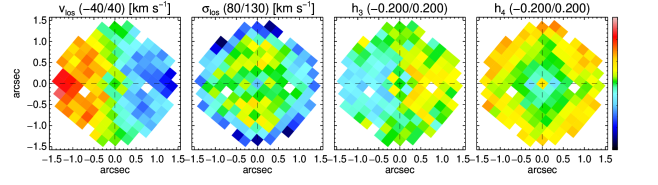
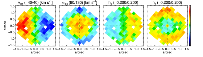
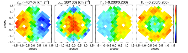
Figure 13.— Maps of fits to the NIFS line-of-sight velocity ($V_{\rm los}$), velocity dispersion ($\sigma_{\rm los}$) and the 3rd and 4th Gauss-Hermite (GH) moments ($h_{3},h_{4}$) for ${{\mathrm{M}}_{\rm BH}\,}=5\times 10^{7}~{}{{\mathrm{M}}_{\odot}},\Upsilon_{H}=0.3~{}{{\mathrm{M}}_{\odot}}/{{\mathrm{L}}_{\odot}}$ with $N_{c}=1240$, $N_{o}=15092$ orbits (top row) and for ${{\mathrm{M}}_{\rm BH}\,}=7.28\times 10^{7}~{}{{\mathrm{M}}_{\odot}},\Upsilon_{H}=0.312~{}{{\mathrm{M}}_{\odot}}/{{\mathrm{L}}_{\odot}}$ $N_{c}=1240$, $N_{o}=15092$ orbits (middle row). The bottom row shows the model velocity fields obtained when only NIFS constraints are included in the fit (${{\mathrm{M}}_{\rm BH}\,}=4.16\times 10^{7}~{}{{\mathrm{M}}_{\odot}},\Upsilon_{H}=0.312~{}{{\mathrm{M}}_{\odot}}/{{\mathrm{L}}_{\odot}}$, $N_{c}=960$, $N_{o}=9936$). These maps should be compared with the bi-symmetrized velocity fields in the bottom panels of Fig. 2.

Figure 13 shows examples of model fits to the 2 dimensional NIFS velocity fields (from left to right $V_{\rm los}$, $\sigma_{\rm los}$, and the GH moments $h_{3}$ and $h_{4}$) for the edge-on ($i=90^{\circ}$) case with $N_{o}=15092$. Note that while the best-fit solutions listed in Tables 2 & 3 are determined by marginalizing over one parameter in the 2D contour surface (which itself is smoothed with a kernel), the 2D grid of models is discrete. The derived best-fit value (shown as stars on the 2D $\chi^{2}$ maps of Figs. 7 and 9) does not overlap with any model on the grid, but lies between 4 grid points. We therefore show velocity fields and 1D kinematics for the model whose parameters are closest to the best-fit solution.

In Figure 13, the top row shows velocity fields for ${{\mathrm{M}}_{\rm BH}\,}=5\times 10^{7}~{}{{\mathrm{M}}_{\odot}},\Upsilon_{H}=0.3~{}{{\mathrm{M}}_{\odot}}/{{\mathrm{L}}_{\odot}}$ (the model closest to the best-fit obtained with $\chi^{2}_{\rm all}$  for $N_{o}=15092$) and the middle row shows velocity fields for ${{\mathrm{M}}_{\rm BH}\,}=7.28\times 10^{7}~{}{{\mathrm{M}}_{\odot}}$, $\Upsilon_{H}=0.312~{}{{\mathrm{M}}_{\odot}}/{{\mathrm{L}}_{\odot}}$ (the model closest to the best-fit obtained with $\chi^{2}_{\rm kin}$  for $N_{o}=15092$). (The bottom row of this figure is for a model with ${{\mathrm{M}}_{\rm BH}\,}=4.16\times 10^{7}~{}{{\mathrm{M}}_{\odot}}$, $\Upsilon_{H}=0.312~{}{{\mathrm{M}}_{\odot}}/{{\mathrm{L}}_{\odot}}$, obtained when only NIFS kinematical data are fitted, and will be discussed in Section 5.3.2.)

The fitted velocity in Figure 13 should be compared with the bi-symmetrized velocity fields in the bottom row of Figure 2. The four white pixels in each panel of the figure were not fitted because it was determined that their extremely high velocity dispersion values ($>130$ ${\mathrm{km\,s^{-1}}}$) were spurious (see Fig. 2) since their values were larger than the central velocity dispersion despite being far from the center.

In Figure 13 the odd-moments of the LOSVD ($V_{\rm los}$, $h_{3}$) are fairly well fitted by both the low ${{\mathrm{M}}_{\rm BH}\,}$ model (top row) and the high ${{\mathrm{M}}_{\rm BH}\,}$ model (middle row). However, the NIFS velocity dispersion $\sigma_{\rm los}$ for the model with ${{\mathrm{M}}_{\rm BH}\,}=5\times 10^{7}~{}{{\mathrm{M}}_{\odot}}$, $\Upsilon_{H}=0.3~{}{{\mathrm{M}}_{\odot}}/{{\mathrm{L}}_{\odot}}$ (top row) is much lower than $\sigma_{\rm los}$ in the data (bottom of Fig. 2). The model with the larger value of ${{\mathrm{M}}_{\rm BH}\,}=7.28\times 10^{7}~{}{{\mathrm{M}}_{\odot}}$ does a slightly better job of reproducing the higher $\sigma_{\rm los}$ values within $\pm 0\farcs 5$, but fails to fit the $\sigma_{\rm los}$ at the edges of the NIFS field, where model values are significantly lower (i.e. bluer pixel colors) than the observed values seen in Figure 2 (bottom). This is because $\sigma_{\rm los}$ from NIFS in the inner 1$\farcs$5 region is overall larger than that obtained with KPNO (${{\mathrm{\sigma}}_{\rm los}}\sim 75$ ${\mathrm{km\,s^{-1}}}$) and MMT (${{\mathrm{\sigma}}_{\rm los}}\sim 90$ ${\mathrm{km\,s^{-1}}}$). Inconsistent velocity dispersion values in the same physical region drives the solution to fit the data with the smallest error bars (i.e., MMT data) thereby under-estimating $\sigma_{\rm los}$ from NIFS. Also note that neither model is able to fit both the low central and high outer $h_{4}$ values seen in the bi-symmetrized NIFS velocity fields (Fig. 2 bottom row, right-most panel).

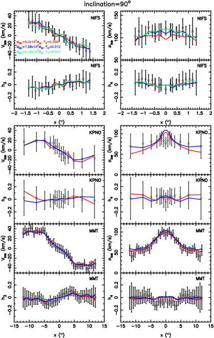
Figure 14.— Fit to observed kinematics $V_{\rm los}$, $\sigma_{\rm los}$, $h_{3}$, $h_{4}$ for: NIFS apertures along the kinematic major axis (top four panels), KPNO slit (middle four panels), and MMT slit (bottom four panels), for inclination angle $i=90^{\circ}$. Curves show fits for three different models with ${{\mathrm{M}}_{\rm BH}\,}$ and $\Upsilon_{H}$ values of: $5\times 10^{7}~{}{{\mathrm{M}}_{\odot}}$ and $0.30~{}{{\mathrm{M}}_{\odot}}/{{\mathrm{L}}_{\odot}}$ (red); $7.28\times 10^{7}~{}{{\mathrm{M}}_{\odot}}$ and $0.312~{}{{\mathrm{M}}_{\odot}}/{{\mathrm{L}}_{\odot}}$ (blue); $4.16\times 10^{7}~{}{{\mathrm{M}}_{\odot}}$ and $0.312~{}{{\mathrm{M}}_{\odot}}/{{\mathrm{L}}_{\odot}}$ (green, fit to NIFS kinematics only).

The difference between the model fits and the data is more clearly seen in Figure 14 which shows the one-dimensional line-of-sight velocity ($V_{\rm los}$), velocity dispersion ($\sigma_{\rm los}$) and the GH moments of the LOSVD ($h_{3}$ and $h_{4}$) that we obtain for the edge-on ($i=90^{\circ}$) model. The red and blue curves show the best fits for same models as in the top and middle panels of Figure 13 with values M_BH and $\Upsilon_{H}$ indicated by the line legends in the top left panel of the first row (these two models used libraries with $N_{o}=15092$ orbits). The green curves in the top four NIFS panels are obtained when only the NIFS data are fitted (with $N_{o}=9936$), this model is discussed in the next section.

The open circles in the panels show the three different kinematic datasets used in the modeling, along with their 1$\sigma$ uncertainties. (The top four panels show kinematics in the NIFS spaxels lying closest to the major axis of the model; the middle four panels show data from the KPNO long-slit; the bottom four panels show data from the MMT long-slit.)

The most striking feature of the fits is that the red curve for ${{\mathrm{M}}_{\rm BH}\,}=5\times 10^{7}~{}{{\mathrm{M}}_{\odot}},\Upsilon_{H}=0.3~{}{{\mathrm{M}}_{\odot}}/{{\mathrm{L}}_{\odot}}$ (red curve) — the model closest to the best-fit solution derived from the minimum in $\chi^{2}_{\rm all}$ (from Figure. 8) — clearly underestimates the NIFS velocity dispersion (top right panel) for the central-most points. The uniformly large central $\sigma_{\rm los}$ values in the inner $\pm 1\arcsec$ region are much better fitted by larger values of ${{\mathrm{M}}_{\rm BH}\,}=7.28\times 10^{7}{{\mathrm{M}}_{\odot}}$ and $\Upsilon_{H}=0.312~{}{{\mathrm{M}}_{\odot}}/{{\mathrm{L}}_{\odot}}$ (blue curve). Both the models do an equally good job of fitting $V_{\rm los}$, $\sigma_{\rm los}$, and $h_{3}$ from the MMT data, but overestimate $\sigma_{\rm los}$ from the KPNO data.

Another important point to note is that the values of the GH parameters $h_{4}$ are negative in the innermost regions of each of the three datasets. Neither model is able to fit the negative $h_{4}$ values measured with the MMT spectrograph nor the central dips to negative values in $h_{4}$ seen in the NIFS data and KPNO data.

In spherical and axisymmetric galaxies, $h_{4}$ is negative when the velocity distribution is tangentially biased; it is positive when orbits are predominantly radial; and it is zero when the velocity distribution in isotropic (van der Marel & Franx, 1993; Gerhard, 1993). However, negative $h_{4}$ values have also been associated specifically with the presence of a bar. In recent $N$-body simulations of barred galaxies by Brown et al. (2013), the LOSVDs have negative $h_{4}$ values in the region where the bar dominates. The negative $h_{4}$ parameters arise due to the kinematic properties of the special orbits that constitute the bar, and due to the fact that from an external observer’s point of view, the bar has a large tangential velocity component due to its pattern speed. Even after a bar buckles and forms a boxy bulge, negative $h_{4}$ values can be seen in face-on systems (Debattista et al., 2005).

Another signature of the kinematics associated with a nuclear bar is undulations in the rising part of the inner rotation curve Bureau & Athanassoula (2005), which we also see in the MMT data for NGC 4151. Finally, while $h_{3}$ is always anti-correlated with the line-of-sight velocity $V_{\rm los}$ in axisymmetric systems, Bureau & Athanassoula (2005) show that $h_{3}$ is correlated with $V_{\rm los}$ along the major axis of the bar. For the data obtained with KPNO (where the slit lies along the major axis of the large scale bar) $h_{3}$ is correlated with $V_{\rm los}$ over the radial range $\pm 2\arcsec$ (Figure 14), providing additional kinematical evidence for a bar.

Therefore it appears that despite the very circular photometric contours of the bulge in NGC 4151, and the visual appearance of a rather weak bar at radii outside the bulge, there are several clear kinematical signatures of a small scale bar in the vicinity of the nuclear BH. This is consistent with the properties of “barlens” features that have recently been identified in real and simulated galaxies (Laurikainen et al., 2011; Athanassoula et al., 2014). As pointed out by Athanassoula et al. (2014), barlenses frequently masquerade as classical bulges because of their nearly circular central isophotes, especially when viewed nearly face-on, but have bar-like kinematics.

The combination of bars and BHs can have significant implications for the central dynamics of galaxies. Brown et al. (2013) analyze a suite of $N$-body simulations of barred galaxies in which point masses representing BHs were grown adiabatically. They find that the growth of a BH of a given mass causes a 5-10% larger increase in $\sigma_{\rm los}$ in a barred galaxy than in an otherwise identical axisymmetric galaxy. Hartmann et al. (2013) find that if a disk galaxy with a bulge has a pre-existing black hole, the formation and evolution of a bar can result in a 15-40% increase in the central velocity dispersion. Both studies find that the increase in the observed line-of-sight velocity dispersion in the barred systems is a consequence of three separate factors: (a) mass inflow due to angular momentum transport by the bar, (b) velocity anisotropy due to the presence of bar orbits, and (c) weak dependence on orientation of position angle of the bar.

If NGC 4151 does have a bar and is thus non-axisymmetric, that fact also has implications for our modeling results. In stellar dynamical modeling of axisymmetric galaxies, fitting a negative $h_{4}$ requires a larger fraction of tangential orbits, which contribute little to the line-of-sight velocity dispersion. Fitting a given velocity dispersion with such an orbit population will imply a larger enclosed mass than would be required if $h_{4}$ was zero or positive (which is typically the case in axisymmetric systems with BHs). Brown et al. (2013) argue that if an axisymmetric stellar dynamical modeling code is used to derive the value of ${{\mathrm{M}}_{\rm BH}\,}$ in a barred galaxy with a high central ${{\mathrm{\sigma}}_{\rm los}}$ and a negative $h_{4}$, the central BH mass will be systematically overestimated. If the large values of ${{\mathrm{\sigma}}_{\rm los}}$ in the nuclear regions and the negative $h_{4}$ values in the MMT data are a consequence a nuclear bar, then the discrepancy between ${{\chi^{2}}_{\rm kin}}$ and ${{\chi^{2}}_{\rm all}}$ could reflect this predicted bias in ${{\mathrm{M}}_{\rm BH}\,}$.

5.3.2 Restricting to Constraints from NIFS

In this section we examine the consequences of fitting only the NIFS kinematical data (ignoring the kinematical constraints at larger radii obtained from the lower spatial resolution long-slit spectra from KPNO and MMT). There are three reasons why the NIFS data alone may provide better constraints on the mass of the BH.

First, the NIFS data have higher spatial resolution (0$\farcs$2) than the long slit data (1″-2″). For a ${{\mathrm{M}}_{\rm BH}\,}\sim 5\times 10^{7}~{}{{\mathrm{M}}_{\odot}}$, the sphere-of-influence of the BH (assuming $\sigma_{c}=116$ ${\mathrm{km\,s^{-1}}}$; see Section 5.4 below) is $\sim$16 pc, which corresponds to $\sim$ 0$\farcs$24 for our assumed distance of 13.9 Mpc for this galaxy. Therefore the NIFS data used in our modeling are barely able to resolve the sphere-of-influence of the BH, but are quite close to doing so. If ${{\mathrm{M}}_{\rm BH}\,}\sim 7.5\times 10^{7}~{}{{\mathrm{M}}_{\odot}}$, the sphere-of-influence of the BH would be 26 pc (0$\farcs$38) and the BH sphere-of-influence would be resolved by the NIFS data. The long slit data do not provide constraints on ${{\mathrm{M}}_{\rm BH}\,}$ and are included mainly to provide constraints on the mass-to-light ratio of the stars, which is assumed to be independent of radius.

Second, as discussed previously, the NIFS velocity dispersion within $\pm 2\arcsec$ is significantly larger than the velocity dispersion on same physical scale obtained from the long-slit data. However, since the error bars on the long-slit MMT data are about half those from the NIFS data, the optimization code tries to fit them better than the NIFS data.

In Figure 13 (top two panels), the need to fit the lower velocity dispersion values from MMT manifests as low velocity dispersion values (blue) at the edges of the NIFS field. These low dispersion values outside the sphere-of-influence of the BH also force the model to adopt a lower mass-to-light ratio, which is then compensated for in the inner region by requiring a much larger M_BH to fit the NIFS velocity dispersion. Neglecting the long-slit data would allow the optimization code to raise the mass-to-light ratio in the inner $\pm$2″ region (where the velocity dispersion is quite flat).

Finally, in Figure 14, we see kinematic evidence for the bar in MMT and KPNO long-slit data (negative $h_{4}$ values and undulations in the rising part of the rotation curve seen in MMT data; correlation between $h_{3}$ and ${{\mathrm{V}}_{\rm los}}$ in KPNO data) occurring on scales of 3″-5″, well outside the nuclear region. Except for the central value of $h_{4}$ in the NIFS dataset (which, as we see from Fig. 1, is contaminated by the AGN), all the other $h_{4}$ values are positive, which is what is expected for orbits around a central BH. Neglecting the long-slit kinematical data could help overcome biases introduced by the bar kinematics. Assuming that the BH mass should primarily be constrained by kinematic constraints at the smallest radii we now test the effect of not including the long-slit data in the NNLS optimization problem. The expectation is that neglecting the long-slit data should bring the best-fit solutions obtained from $\chi^{2}_{\rm all}$ and $\chi^{2}_{\rm kin}$ closer to each other.

We construct a full sets of models (18 values of ${{\mathrm{M}}_{\rm BH}\,}$ and 18 values of $\Upsilon_{H}$) in which we only fitted the nuclear kinematical data obtained with the NIFS spectrograph, with an orbit library of $N_{o}=9936$. Figure 15 shows $\Delta\chi^{2}$ values obtained by marginalizing over $\Upsilon_{H}$ (top) and by marginalizing over ${{\mathrm{M}}_{\rm BH}\,}$ (middle). The solid curves show $\Delta\chi^{2}_{\rm all}$ while the dashed curves show $\Delta\chi^{2}_{\rm kin}$. The dotted horizontal lines show the 1$\sigma$, 2$\sigma$ and 3$\sigma$ confidence levels, respectively (for 1 degree-of-freedom). The top plot shows that the minimum $\chi^{2}_{\rm kin}$ (dashed curve) has decreased quite significantly and is now in agreement with the minimum $\chi^{2}_{\rm all}$ (solid curve). The best-fit values of $\Upsilon_{H}$ (middle panel) are still inconsistent within 1$\sigma$ but are consistent within 3$\sigma$. The bottom-most panel shows the error on the fit to the mass and surface brightness distribution. Contours are spaced at intervals of 0.1% error per constraint. It is clear that the fit to the self-consistency constraints is uniform over a much larger range of ${{\mathrm{M}}_{\rm BH}\,}$ and $\Upsilon_{H}$ values implying that the fit to the mass is no longer a significant factor in determining the location of the minimum.

The best fit black hole mass and M/L ratio obtained using $\Delta\chi^{2}_{\rm all}$ and $\Delta\chi^{2}_{\rm kin}$, along with the reduced $\Delta\chi^{2}$ and 1$\sigma$ and 3$\sigma$ error bars, are shown in the bottom two rows of Table 3. Since the best fit ${{\mathrm{M}}_{\rm BH}\,}$ values and their 1$\sigma$ error bars from both methods of computing $\chi^{2}$ are nearly the same we use the average of the two best-fit values as the solution and sum their 1$\sigma$ errors in quadrature to obtain ${{\mathrm{M}}_{\rm BH}\,}=3.76\pm 1.15$. Figure 15 shows that the $\Upsilon_{H}$ values obtained from $\chi^{2}_{\rm kin}$ are consistent with the best fit value obtained with $\chi^{2}_{\rm all}$ at the 3$\sigma$ level, but both are well within the expected range $0.4\pm 0.2~{}{{\mathrm{M}}_{\odot}}/{{\mathrm{L}}_{\odot}}$. Therefore we use the average of the two best-fit M/L values and sum their 3$\sigma$ errors in quadrature to get $\Upsilon_{H}=0.34\pm 0.03$.

The bottom panel of Figure 13 shows a 2D kinematic map for a model with ${{\mathrm{M}}_{\rm BH}\,}=4.16\times 10^{7}~{}{{\mathrm{M}}_{\odot}}$ and $\Upsilon=0.312~{}{{\mathrm{M}}_{\odot}}/{{\mathrm{L}}_{\odot}}$, with parameters closest to the best-fit solution obtained with ${{\chi^{2}}_{\rm all}}$ (see 3rd row of Table 3). This model achieves adequately large values of ${{\mathrm{\sigma}}_{\rm los}}$ (see red/orange regions) over the central NIFS field by raising the M/L ratio very slightly from $\Upsilon=0.3$ to $\Upsilon=0.312$. The 1D kinematic fit of this model to the NIFS data along the kinematic major axis of the model is shown by the green curves in Figure 14, from which it is also clear that the lower value of ${{\mathrm{M}}_{\rm BH}\,}$ is able to fit the high velocity dispersion values even better than the high BH mass when the model attempted to fit both the NIFS and long-slit kinematic data.

This test largely confirms our hypothesis that the two main causes of the large value of ${{\mathrm{M}}_{\rm BH}\,}$ obtained in the previous section were (a) inconsistencies between ${{\mathrm{\sigma}}_{\rm los}}$ values from NIFS and the long-slit data in the same spatial region, (b) the need to fit the low $h_{4}$ values and high central ${{\mathrm{\sigma}}_{\rm los}}$ values with a low M/L ratio. Thus, we see that by not including the kinematics data with poorer spatial resolution (which are clearly unaffected by the BH as can be seen in Figure 13) we are able to simultaneously fit the NIFS kinematics and the mass and surface brightness distributions with a lower value of ${{\mathrm{M}}_{\rm BH}\,}$.

Figure 15.— Results of fitting NIFS kinematics only. 1D $\Delta\chi^{2}$ obtained by marginalizing over $\Upsilon_{H}$ (top) and marginalizing over ${{\mathrm{M}}_{\rm BH}\,}$ (middle) for models constructed using an orbit library of $N_{o}=9936$ orbits. $\Delta{{\chi^{2}}_{\rm all}}$ is shown by solid curves and $\Delta{{\chi^{2}}_{\rm kin}}$ is shown by dashed curves. The bottom-most panel shows errors on the fit to the mass distribution (contours are spaced at 0.1% error per constraint). Mass fit errors are uniform over a larger range of parameters and hence contribute negligibly to ${{\chi^{2}}_{\rm all}}$.

5.4. The $M_{\rm BH}-\sigma$ Relation

In this section, we determine how the new NIFS kinematic measurements in the nuclear region of NGC 4151 affect the galaxy’s location in the $M_{\rm BH}-\sigma$ relation. The aperture used to define the appropriate $\sigma$ value for the relation is a historically contentious issue (e.g. Merritt & Ferrarese, 2001; Tremaine et al., 2002), but the NIFS data naturally lend themselves to one of those standards: $\sigma_{c}$, which is the velocity dispersion within an aperture of radius $R_{e}$/8, where $R_{e}$ is the bulge effective radius (Ferrarese & Merritt, 2000). (Despite having to adopt one particular standard, we note that Merritt & Ferrarese (2001) found no systematic differences between estimates of $\sigma_{c}$ (inside of $R_{e}$/8) and estimates of $\sigma$ that extended out to $R_{e}$, likely because of the steep radial surface brightness gradient in most bulges.) The $R_{e}$ value for NGC 4151 has been measured to be $\approx 10\arcsec$ (Dong & De Robertis, 2006; Bentz et al., 2009; Weinzirl et al., 2009), while the NIFS field-of-view extends to a radius of between $1\farcs 5$ and $2\farcs 1$. Thus, we sum the NIFS datacube across all of the spaxels into a single spectrum, and fit for the dispersion using pPXF.

From the NIFS data, we find $\sigma_{c}=116\pm 3$ ${\mathrm{km\,s^{-1}}}$. This is somewhat larger than either the $89\pm 13$ ${\mathrm{km\,s^{-1}}}$ measured by Ferrarese et al. (2001), or the $97\pm 3$ ${\mathrm{km\,s^{-1}}}$ measured by Nelson et al. (2004). Both of those earlier measurements used the Calcium triplet absorption lines, but whereas the former covered a similar region of the galaxy as our NIFS spectra ($2\arcsec\times 4\arcsec$), the latter used an aperture of $1\arcsec\times 6\farcs 5$. Previous studies of bulge kinematics have found near-IR and optical data to give consistent results (see Kang et al., 2013, and references therein), while the discrepancies seen in some luminous IR galaxies are in the sense of smaller $\sigma$ values from the CO-bandheads (Rothberg et al., 2013).

Our new measurement of $\sigma_{c}=116\pm 3$ ${\mathrm{km\,s^{-1}}}$ is $\sim$25% above the previous velocity dispersion measurements, while our best-fit stellar dynamical estimate of $\sim 3.76\pm 1.15\times 10^{7}~{}{{\mathrm{M}}_{\odot}}$ is 17% below our earlier stellar dynamical estimate (Onken et al., 2007). Previously, NGC 4151 had been an outlier from the AGN $M_{\rm BH}-\sigma$ relation in the direction of low-$\sigma$ or high-${{\mathrm{M}}_{\rm BH}\,}$. The new $\sigma_{c}$ and ${{\mathrm{M}}_{\rm BH}\,}$ measurements helps to bring NGC 4151 closer to the best-fit relation of Woo et al. (2013), though it does remain on the low-$\sigma$ side.

Finally, we note that if the BH masses in barred galaxies have been overestimated due to the use of axisymmetric dynamical modeling codes, such galaxies would lie even further below the standard M${}_{\rm BH}-\sigma$ relation than has been found previously (Graham et al., 2011, and references therein). This demonstrates the importance of developing robust bar dynamical modeling approaches in the future.

6. Summary and Discussion

We have conducted AO-assisted near-IR integral field spectroscopy of the local Seyfert galaxy NGC 4151, using the NIFS instrument on Gemini North. We used an axisymmetric orbit-superposition code to fit the observed surface brightness distribution within 50″, NIFS kinematics within $\pm$1$\farcs$5, and long slit kinematics along two different position angles in order to estimate the best-fit values of the mass of the BH (${{\mathrm{M}}_{\rm BH}\,}$) and the mass-to-light ratio of the stars ($\Upsilon_{H}$). Models were constructed for 10-18 values of ${{\mathrm{M}}_{\rm BH}\,}$, 18 values of $\Upsilon_{H}$ and 3 different inclination angles. The main results of this paper are summarized below.

We use the $\chi^{2}$ estimator to determine the model which gives the best-fit to the data but find that the solution depends on whether the $\chi^{2}$ includes both self-consistency constraints (which are not strictly speaking “data”) and kinematic constraints or only kinematic constraints. When we use both types of constraints and all the available kinematical data (from low-resolution long-slit data and high resolution NIFS data) the best-fit solution is ${{\mathrm{M}}_{\rm BH}\,}=4.68\times 10^{7}~{}{{\mathrm{M}}_{\odot}}$ and $\Upsilon_{H}\sim 0.30{{\mathrm{M}}_{\odot}}/{{\mathrm{L}}_{\odot}}$, for a model with $i=90^{\circ}$. However, this best fit model gives a central ${{\mathrm{\sigma}}_{\rm los}}$ that is too low to fit the data obtained with the NIFS instrument. When we use ${{\chi^{2}}_{\rm kin}}$ (determined by only considering the fit to the kinematic data), the best fit model has ${{\mathrm{M}}_{\rm BH}\,}=7.32\times 10^{7}~{}{{\mathrm{M}}_{\odot}}$ and $\Upsilon_{H}\sim 0.31~{}{{\mathrm{M}}_{\odot}}/{{\mathrm{L}}_{\odot}}$, and provides a better fit to the nuclear kinematical data from NIFS spectrograph, although it gives a slightly worse fit to the mass and surface brightness distributions.

An interesting point worth noting is that Hicks & Malkan (2008) found a best-fit value of ${{\mathrm{M}}_{\rm BH}\,}=3^{+0.75}_{-2.2}\times 10^{7}$ in NGC 4151 when they fitted the kinematics of the H₂ line-emitting gas within 1″ of the center (see Figure 43 in their paper). However, if they included the kinematics of gas within 2″ they obtained a larger value of ${{\mathrm{M}}_{\rm BH}\,}\sim 8\times 10^{7}~{}{{\mathrm{M}}_{\odot}}$, although with a somewhat worse reduced-$\chi^{2}$. It is intriguing that both our stellar dynamical modeling and their gas dynamical modeling, while preferring lower values of ${{\mathrm{M}}_{\rm BH}\,}\sim 3-5\times 10^{7}$, also suggest that higher values of ${{\mathrm{M}}_{\rm BH}\,}$ may be obtained when lower spatial resolution data are included in the fit.

Models are generated for three different inclination angles of the bulge $i=23^{\circ},60^{\circ},90^{\circ}$ and show that the best-fit ${{\mathrm{M}}_{\rm BH}\,}$ and $\Upsilon_{H}$ values are relatively insensitive to inclination angle. We examine an additional 4 inclination angles for fixed BH mass values (${{\mathrm{M}}_{\rm BH}\,}=5\times 10^{7},10^{8}$) and fixed mass-to-light ratio ($\Upsilon_{H}=0.3$). We find that edge-on models ($i=90^{\circ}$) give the smallest $\chi^{2}$ values, while models with the inclination of the large scale disk ($i=23^{\circ}$) are strongly disfavored. This suggests that the bulge must be nearly spherical but its rotation axis is significantly misaligned from the rotation axis of the disk. However, it is well known from previous work (Krajnović et al., 2005; Lablanche et al., 2012) that inclination of a spheroid is extremely difficult to determine via dynamical modelling, especially in the presence of a bar. This determination of the inclination of the bulge should therefore be treated with caution.

A detailed examination of the kinematics in the inner 5″ of NGC 4151 shows evidence for bar kinematics, which manifest as high values of ${{\mathrm{\sigma}}_{\rm los}}$, low or negative values of $h_{4}$ and $h_{3}$ values which are correlated with ${{\mathrm{V}}_{\rm los}}$. We hypothesize that the discrepancy between the $\chi^{2}$ obtained from including all the constraints and that obtained by only including the kinematic constraints is likely a consequence of two factors: (a) a stellar bar, which is not possible to model with our axisymmetric code, and (b) inconsistencies between the velocity dispersion values obtained from the low-spatial resolution long-slit data and the high spatial resolution NIFS data over the same spatial range. This hypothesis was tested by fitting only the NIFS data.

When we fit only the kinematical data obtained with the NIFS spectrograph (neglecting all kinematical constraints beyond $\pm 1\farcs 5$ - i.e those data that show kinematical evidence for a bar and data that is discrepant with high-resolution NIFS data), the non-negative optimization problem was able to find a much better fit to the NIFS data and the same best-fit ${{\mathrm{M}}_{\rm BH}\,}$ was obtained by both methods of computing $\chi^{2}$.

The stellar-dynamical modeling carried out in this paper gives a best-fit value of ${{\mathrm{M}}_{\rm BH}\,}=3.76\pm 1.15\times 10^{7}{{\mathrm{M}}_{\odot}}\,$ (obtained by averaging over the ${{\chi^{2}}_{\rm all}}$ and ${{\chi^{2}}_{\rm kin}}$ values in the lower two rows of Table 3) which is consistent at the 1$\sigma$ level with the reverberation mapping-based mass of $3.57^{+0.45}_{-0.37}\times 10^{7}~{}{{\mathrm{M}}_{\odot}}$ (1$\sigma$ errors) obtained by using data from Bentz et al. (2006), but relying on a recently updated empirical calibration of the RM mass scale by Grier et al. (2013). The best fit M/L ratio $\Upsilon_{H}=0.34\pm 0.03$ (3$\sigma$ error) is consistent with the photometrically derived mass-to-light ratio of $\Upsilon_{H}=0.4{\pm 0.2}~{}{{\mathrm{M}}_{\odot}}/{{\mathrm{L}}_{\odot}}$.

The new NIFS data yields $\sigma_{c}=116\pm 3$${\mathrm{km\,s^{-1}}}$, the velocity dispersion within $R_{e}/8$, which is $\sim$25% larger than previous values, while the new best estimate of ${{\mathrm{M}}_{\rm BH}\,}=3.76\pm 1.15\times 10^{7}~{}{{\mathrm{M}}_{\odot}}$ 17% smaller than but fully consistent with both our previous stellar dynamical upper limit (Onken et al., 2007) and the dynamical estimate based on H₂ line-emitting gas (Hicks & Malkan, 2008). The larger value of $\sigma_{c}$ and smaller value of ${{\mathrm{M}}_{\rm BH}\,}$ help to bring NGC 4151 closer to the best-fit M${}_{\rm BH}-\sigma$ relation of Woo et al. (2013).

The analysis in this paper demonstrates that biased estimates of BH masses can arise when an axisymmetric orbit superposition code is used to model a galaxy with a weak, but kinematically identifiable barred galaxy, possibly resulting in an over-estimate in ${{\mathrm{M}}_{\rm BH}\,}$ if the M/L ratio is constrained primarily by data beyond the sphere-of-influence of the BH. This confirms the prediction made from the recent analysis of $N$-body simulations of barred galaxies with BHs by Brown et al. (2013), and points to the need for new dynamical modeling tools capable of modeling a stellar bar. When such codes are applied to the existing sample of barred galaxies, our results suggest that it will likely enhance the discrepancy between barred and unbarred galaxies in the $M_{\rm BH}-\sigma$ relation (Graham et al., 2011).

Our modeling of this complex system suggests that the standard practice of fitting kinematical constraints over a large range of radii with a constant mass-to-light ratio (for exceptions to this practice, see Valluri et al., 2005; McConnell et al., 2013) can bias the mass of the central BH and the derived mass-to-light ratio. To some extent, the biases can be overcome by only considering the kinematics very close to the central BH, although this gives larger errors on the estimated solutions of ${{\mathrm{M}}_{\rm BH}\,}$ and $\Upsilon_{H}$. Our tests of robustness demonstrate that the use of such high spatial resolution nuclear kinematical data in such modeling is very valuable. However, the complications of the stellar dynamical bar imply that additional work is required in order to perform the crucial test of the RM mass scale calibration in this galaxy. Only with improved non-axisymmetric modeling methods and/or BH mass measurements in other reverberation-mapped AGNs will we ultimately be able to assess whether the growth history of the BHs that we see accreting at present is systematically different from those currently in quiescence.

References

- Athanassoula et al. (2014) Athanassoula, E., Laurikainen, E., Salo, H., & Bosma, A. 2014, MNRAS, submitted (arXiv:1405.6726)
- Barth et al. (2002) Barth, A. J., Ho, L. C., & Sargent, W. L. W. 2002, AJ, 124, 2607
- Bentz et al. (2006) Bentz, M. C., Denney, K. D., Cackett, E. M., Dietrich, M., Fogel, J. K. J., Ghosh, H., Horne, K., Kuehn, C., Minezaki, T., Onken, C. A., Peterson, B. M., Pogge, R. W., Pronik, V. I., Richstone, D. O., Sergeev, S. G., Vestergaard, M., Walker, M. G., & Yoshii, Y. 2006, ApJ, 651, 775
- Bentz et al. (2009) Bentz, M. C., Walsh, J. L., Barth, A. J., Baliber, N., Bennert, V. N., Canalizo, G., Filippenko, A. V., Ganeshalingam, M., Gates, E. L., Greene, J. E., Hidas, M. G., Hiner, K. D., Lee, N., Li, W., Malkan, M. A., Minezaki, T., Sakata, Y., Serduke, F. J. D., Silverman, J. M., Steele, T. N., Stern, D., Street, R. A., Thornton, C. E., Treu, T., Wang, X., Woo, J.-H., & Yoshii, Y. 2009, ApJ, 705, 199
- Bentz et al. (2010) Bentz, M. C., Walsh, J. L., Barth, A. J., Yoshii, Y., Woo, J.-H., Wang, X., Treu, T., Thornton, C. E., Street, R. A., Steele, T. N., Silverman, J. M., Serduke, F. J. D., Sakata, Y., Minezaki, T., Malkan, M. A., Li, W., Lee, N., Hiner, K. D., Hidas, M. G., Greene, J. E., Gates, E. L., Ganeshalingam, M., Filippenko, A. V., Canalizo, G., Bennert, V. N., & Baliber, N. 2010, ApJ, 716, 993
- Binney & Merrifield (1998) Binney, J. & Merrifield, M. 1998, Galactic Astronomy (Princeton University Press, Princeton, NJ)
- Binney & Tremaine (2008) Binney, J. & Tremaine, S. 2008, Galactic Dynamics: Second Edition (Princeton University Press)
- Blandford & McKee (1982) Blandford, R. D. & McKee, C. F. 1982, ApJ, 255, 419
- Boccas et al. (2006) Boccas, M., Rigaut, F., Bec, M., et al. 2006, Proc. SPIE, 6272
- Bon et al. (2012) Bon, E., Jovanović, P., Marziani, P., Shapovalova, A. I., Bon, N., Borka Jovanović, V., Borka, D., Sulentic, J., & Popović, L. Č. 2012, ApJ, 759, 118
- Brown et al. (2013) Brown, J. S., Valluri, M., Shen, J., & Debattista, V. P. 2013, ApJ, 778, 151
- Bruzual & Charlot (2003) Bruzual, G., & Charlot, S. 2003, MNRAS, 344, 1000
- Bureau & Athanassoula (2005) Bureau, M. & Athanassoula, E. 2005, ApJ, 626, 159
- Cappellari (2002) Cappellari, M. 2002, MNRAS, 333, 400
- Cappellari & Emsellem (2004) Cappellari, M. & Emsellem, E. 2004, PASP, 116, 138
- Crenshaw et al. (2010) Crenshaw, D. M., Schmitt, H. R., Kraemer, S. B., Mushotzky, R. F., & Dunn, J. P. 2010, ApJ, 708, 419
- Cretton et al. (1999) Cretton, N., de Zeeuw, P. T., van der Marel, R. P., & Rix, H.-W. 1999, ApJS, 124, 383
- Das et al. (2005) Das, V., Crenshaw, D. M., Hutchings, J. B., Deo, R. P., Kraemer, S. B., Gull, T. R., Kaiser, M. E., Nelson, C. H., & Weistrop, D. 2005, AJ, 130, 945
- Davies (1973) Davies, R. D. 1973, MNRAS, 161, 25P
- Davies et al. (2006) Davies, R. I., Thomas, J., Genzel, R., Mueller Sánchez, F., Tacconi, L. J., Sternberg, A., Eisenhauer, F., Abuter, R., Saglia, R., & Bender, R. 2006, ApJ, 646, 754
- de Vaucouleurs et al. (1991) de Vaucouleurs, G., de Vaucouleurs, A., Corwin, Jr., H. G., Buta, R. J., Paturel, G., & Fouqué, P. 1991, Third Reference Catalogue of Bright Galaxies. Volume I: Explanations and references. Volume II: Data for galaxies between 0h and 12h. Volume III: Data for galaxies between 12h and 24h. (Springer-Verlag: New York)
- Debattista et al. (2005) Debattista, V. P., Carollo, C. M., Mayer, L., & Moore, B. 2005, ApJ, 628, 678
- Dong & De Robertis (2006) Dong, X. Y. & De Robertis, M. M. 2006, AJ, 131, 1236
- Dumas et al. (2007) Dumas, G., Mundell, C. G., Emsellem, E., & Nagar, N. M. 2007, MNRAS, 379, 1249
- Emsellem et al. (1994) Emsellem, E., Monnet, G., & Bacon, R. 1994, A&A, 285, 723
- Eskridge et al. (2002) Eskridge, P. B., Frogel, J. A., Pogge, R. W., Quillen, A. C., Berlind, A. A., Davies, R. L., DePoy, D. L., Gilbert, K. M., Houdashelt, M. L., Kuchinski, L. E., Ramírez, S. V., Sellgren, K., Stutz, A., Terndrup, D. M., & Tiede, G. P. 2002, ApJS, 143, 73
- Ferrarese & Merritt (2000) Ferrarese, L. & Merritt, D. 2000, ApJ, 539, L9
- Ferrarese et al. (2001) Ferrarese, L., Pogge, R. W., Peterson, B. M., Merritt, D., Wandel, A., & Joseph, C. L. 2001, ApJ, 555, L79
- Gallimore et al. (1999) Gallimore, J. F., Baum, S. A., O’Dea, C. P., Pedlar, A., & Brinks, E. 1999, ApJ, 524, 684
- Gebhardt et al. (2003) Gebhardt, K., Richstone, D., Tremaine, S., Lauer, T. R., Bender, R., Bower, G., Dressler, A., Faber, S. M., Filippenko, A. V., Green, R., Grillmair, C., Ho, L. C., Kormendy, J., Magorrian, J., & Pinkney, J. 2003, ApJ, 583, 92
- Gerhard (1993) Gerhard, O. E. 1993, MNRAS, 265, 213
- Gerhard & Binney (1996) Gerhard, O. E. & Binney, J. J. 1996, MNRAS, 279, 993
- Gillessen et al. (2009) Gillessen, S., Eisenhauer, F., Fritz, T. K., Bartko, H., Dodds-Eden, K., Pfuhl, O., Ott, T., & Genzel, R. 2009, ApJ, 707, L114
- Graham et al. (2011) Graham, A. W., Onken, C. A., Athanassoula, E., & Combes, F. 2011, MNRAS, 412, 2211
- Grier et al. (2013) Grier, C. J., Martini, P., Watson, L. C., Peterson, B. M., Bentz, M. C., Dasyra, K. M., Dietrich, M., Ferrarese, L., Pogge, R. W., & Zu, Y. 2013, ApJ, 773, 90
- Hartmann et al. (2013) Hartmann, M., Debattista, V. P., Cole, D. R., Valluri, M., Widrow, L. M., & Shen, J. 2013, ApJ (submitted) ArXiv e-prints
- Herriot et al. (1998) Herriot, G., Morris, S., Roberts, S., et al. 1998, Proc. SPIE, 3353, 488
- Hicks & Malkan (2008) Hicks, E. K. S. & Malkan, M. A. 2008, ApJS, 174, 31
- Houghton et al. (2006) Houghton, R. C. W., Magorrian, J., Sarzi, M., Thatte, N., Davies, R. L., & Krajnović, D. 2006, MNRAS, 367, 2
- Ivanov et al. (2000) Ivanov, V. D., Rieke, G. H., Groppi, C. E., Alonso-Herrero, A., Rieke, M. J., & Engelbracht, C. W. 2000, ApJ, 545, 190
- Jahnke et al. (2004) Jahnke, K., Wisotzki, L., Sánchez, S. F., et al. 2004, Astronomische Nachrichten, 325, 128
- Joseph et al. (2001) Joseph, C. L., Merritt, D., Olling, R., Valluri, M., Bender, R., Bower, G., Danks, A., Gull, T., Hutchings, J., Kaiser, M. E., Maran, S., Weistrop, D., Woodgate, B., Malumuth, E., Nelson, C., Plait, P., & Lindler, D. 2001, ApJ, 550, 668
- Kang et al. (2013) Kang, W.-R., Woo, J.-H., Schulze, A., Riechers, D. A., Kim, S. C., Park, D., & Smolcic, V. 2013, ApJ, 767, 26
- Kochanek & Rybicki (1996) Kochanek, C. S. & Rybicki, G. B. 1996, MNRAS, 280, 1257
- Krajnović et al. (2005) Krajnović, D., Cappellari, M., Emsellem, E., McDermid, R. M., & de Zeeuw, P. T. 2005, MNRAS, 357, 1113
- Lablanche et al. (2012) Lablanche, P.-Y., Cappellari, M., Emsellem, E., Bournaud, F., Michel-Dansac, L., Alatalo, K., Blitz, L., Bois, M., Bureau, M., Davies, R. L., Davis, T. A., de Zeeuw, P. T., Duc, P.-A., Khochfar, S., Krajnović, D., Kuntschner, H., Morganti, R., McDermid, R. M., Naab, T., Oosterloo, T., Sarzi, M., Scott, N., Serra, P., Weijmans, A.-M., & Young, L. M. 2012, MNRAS, 424, 1495
- Laurikainen et al. (2011) Laurikainen, E., Salo, H., Buta, R., & Knapen, J. H. 2011, MNRAS, 418, 1452
- Lawson & Hanson (1974) Lawson, C. L. & Hanson, R. J. 1974, Solving least squares problems (Prentice-Hall: Englewood Cliffs)
- McConnell et al. (2013) McConnell, N. J., Chen, S.-F. S., Ma, C.-P., Greene, J. E., Lauer, T. R., & Gebhardt, K. 2013, ApJ, 768, L21
- McGregor et al. (2003) McGregor, P. J., Hart, J., Conroy, P. G., Pfitzner, M. L., Bloxham, G. J., Jones, D. J., Downing, M. D., Dawson, M., Young, P., Jarnyk, M., & Van Harmelen, J. 2003, in Society of Photo-Optical Instrumentation Engineers (SPIE) Conference Series, Vol. 4841, Society of Photo-Optical Instrumentation Engineers (SPIE) Conference Series, ed. M. Iye & A. F. M. Moorwood, 1581–1591
- Merritt & Ferrarese (2001) Merritt, D. & Ferrarese, L. 2001, ApJ, 547, 140
- Michell (1784) Michell, J. 1784, Royal Society of London Philosophical Transactions Series I, 74, 35
- Müller-Sánchez et al. (2011) Müller-Sánchez, F., Prieto, M. A., Hicks, E. K. S., Vives-Arias, H., Davies, R. I., Malkan, M., Tacconi, L. J., & Genzel, R. 2011, ApJ, 739, 69
- Nelson et al. (2004) Nelson, C. H., Green, R. F., Bower, G., Gebhardt, K., & Weistrop, D. 2004, ApJ, 615, 652
- Onken et al. (2004) Onken, C. A., Ferrarese, L., Merritt, D., Peterson, B. M., Pogge, R. W., Vestergaard, M., & Wandel, A. 2004, ApJ, 615, 645
- Onken et al. (2007) Onken, C. A., Valluri, M., Peterson, B. M., Pogge, R. W., Bentz, M. C., Ferrarese, L., Vestergaard, M., Crenshaw, D. M., Sergeev, S. G., McHardy, I. M., Merritt, D., Bower, G. A., Heckman, T. M., & Wandel, A. 2007, ApJ, 670, 105 (Paper I)
- Pedlar et al. (1992) Pedlar, A., Howley, P., Axon, D. J., & Unger, S. W. 1992, MNRAS, 259, 369
- Peterson (2001) Peterson, B. M. 2001, in Advanced Lectures on the Starburst-AGN, ed. I. Aretxaga, D. Kunth, & R. Mújica, 3
- Peterson et al. (2004) Peterson, B. M., Ferrarese, L., Gilbert, K. M., Kaspi, S., Malkan, M. A., Maoz, D., Merritt, D., Netzer, H., Onken, C. A., Pogge, R. W., Vestergaard, M., & Wandel, A. 2004, ApJ, 613, 682
- Riffel et al. (2009) Riffel, R. A., Storchi-Bergmann, T., & McGregor, P. J. 2009, ApJ, 698, 1767
- Rothberg et al. (2013) Rothberg, B., Fischer, J., Rodrigues, M., & Sanders, D. B. 2013, ApJ, 767, 72
- Ruiz et al. (2003) Ruiz, M., Young, S., Packham, C., Alexander, D. M., & Hough, J. H. 2003, MNRAS, 340, 733
- Schlegel et al. (1998) Schlegel, D. J., Finkbeiner, D. P., & Davis, M. 1998, ApJ, 500, 525
- Schwarzschild (1979) Schwarzschild, M. 1979, ApJ, 232, 236
- Shimono et al. (2010) Shimono, A., Sugai, H., Kawai, A., Matsubayashi, K., Ohtani, H., Ozaki, S., Hattori, T., & Kosugi, G. 2010, PASJ, 62, 225
- Simkin (1975) Simkin, S. M. 1975, ApJ, 200, 567
- Storchi-Bergmann et al. (2010) Storchi-Bergmann, T., Lopes, R. D. S., McGregor, P. J., Riffel, R. A., Beck, T., & Martini, P. 2010, MNRAS, 402, 819
- Storchi-Bergmann et al. (2009) Storchi-Bergmann, T., McGregor, P. J., Riffel, R. A., Simões Lopes, R., Beck, T., & Dopita, M. 2009, MNRAS, 394, 1148
- Takahashi et al. (2002) Takahashi, K., Inoue, H., & Dotani, T. 2002, PASJ, 54, 373
- Tremaine et al. (2002) Tremaine, S., Gebhardt, K., Bender, R., Bower, G., Dressler, A., Faber, S. M., Filippenko, A. V., Green, R., Grillmair, C., Ho, L. C., Kormendy, J., Lauer, T. R., Magorrian, J., Pinkney, J., & Richstone, D. 2002, ApJ, 574, 740
- Tully et al. (2009) Tully, R. B., Rizzi, L., Shaya, E. J., Courtois, H. M., Makarov, D. I., & Jacobs, B. A. 2009, AJ, 138, 323
- Valluri et al. (2005) Valluri, M., Ferrarese, L., Merritt, D., & Joseph, C. L. 2005, ApJ, 628, 137
- Valluri et al. (2004) Valluri, M., Merritt, D., & Emsellem, E. 2004, ApJ, 602, 66 (VME04)
- van den Bosch & de Zeeuw (2010) van den Bosch, R. C. E. & de Zeeuw, P. T. 2010, MNRAS, 401, 1770
- van den Bosch et al. (2008) van den Bosch, R. C. E., van de Ven, G., Verolme, E. K., Cappellari, M., & de Zeeuw, P. T. 2008, MNRAS, 385, 647
- van der Marel et al. (1998) van der Marel, R. P., Cretton, N., de Zeeuw, P. T., & Rix, H. 1998, ApJ, 493, 613
- van der Marel & Franx (1993) van der Marel, R. P. & Franx, M. 1993, ApJ, 407, 525
- Weinzirl et al. (2009) Weinzirl, T., Jogee, S., Khochfar, S., Burkert, A., & Kormendy, J. 2009, ApJ, 696, 411
- Woo et al. (2013) Woo, J.-H., Schulze, A., Park, D., Kang, W.-R., Kim, S. C., & Riechers, D. A. 2013, ApJ, 772, 49
- Woo et al. (2010) Woo, J.-H., Treu, T., Barth, A. J., Wright, S. A., Walsh, J. L., Bentz, M. C., Martini, P., Bennert, V. N., Canalizo, G., Filippenko, A. V., Gates, E., Greene, J., Li, W., Malkan, M. A., Stern, D., & Minezaki, T. 2010, ApJ, 716, 269
- Zibetti et al. (2009) Zibetti, S., Charlot, S., & Rix, H.-W. 2009, MNRAS, 400, 1181