On Absence and Existence of the Anomalous Localized Resonance without the Quasi-static Approximation

Abstract

The paper considers the transmission problems for Helmholtz equation with bodies that have negative material parameters. Such material parameters are used to model metals on optical frequencies and so-called metamaterials. As the absorption of the materials in the model tends to zero the fields may blow up. When the speed of the blow up is suitable, this is called the Anomalous Localized Reconance (ALR). In this paper we study this phenomenon and formulate a new condition, the weak Anomalous Localized Reconance (w-ALR), where the speed of the blow up of fields may be slower. Using this concept, we can study the blow up of fields in the presence of negative material parameters without the commonly used quasi-static approximation. We give simple geometric conditions under which w-ALR or ALR may, or may not appear. In particular, we show that in a case of a curved layer of negative material with a strictly convex boundary neither ALR nor w-ALR appears with non-zero frequencies (i.e. in the dynamic range) in dimensions $d\geq 3$. In the case when the boundary of the negative material contains a flat subset we show that the w-ALR always happens with some point sources in dimensions $d\geq 2$. These results, together with the earlier results of Milton et al. ( [22, 23]) and Ammari et al. ([2]) show that for strictly convex bodies ALR may appear only for bodies so small that the quasi-static approximation is realistic. This gives limits for size of the objects for which invisibility cloaking methods based on ALR may be used.

University of Helsinki

Department of Mathematics and Statistics

P.O.Box 68, 00014 University of Helsinki, Finland

henrik.kettunen@helsinki.fi, matti.lassas@helsinki.fi, petri.ola@helsinki.fi

1 Introduction and statement of main results

Consider a pair of bounded $C^{\infty}$-domains $D$ and $\Omega$ of $\mathbb{R}^{d}$, $d\geq 2$, such that the closure of $D$ is included in $\Omega$. Given complex wave numbers $k_{\text{e}}$ and $k_{\text{i}}$, ${\rm Im\,}k_{\text{e}},\,{\rm Im\,}k_{\text{i}}\geq 0$, we consider the properties of the following transmission problem

$$-(\Delta+k_{\text{e}}^{2})v_{1} = 0\text{ in }D$$ (1.1)

$$-(\Delta+k_{\text{i}}^{2})v_{2} = 0\text{ in }\Omega\setminus\overline{D}$$

$$-(\Delta+k_{\text{e}}^{2})v_{3} = f\text{ in }\mathbb{R}^{d}\setminus\Omega,\quad f\in{\cal E}^{\prime}(\mathbb{R}^{d}\setminus\overline{\Omega}),$$

where on the interior boundary $\Gamma_{1}=\partial D$ we have the boundary conditions

$$v_{1}|_{\Gamma_{1}}=v_{2}|_{\Gamma_{1}},\quad\tau_{1}\partial_{\nu}v_{1}|_{\Gamma_{1}}=\partial_{\nu}v_{2}|_{\Gamma_{1}}$$ (1.2)

and on the exterior boundary $\Gamma_{2}={\partial\Omega}$ we have

$$v_{2}|_{\Gamma_{2}}=v_{3}|_{\Gamma_{2}},\quad\tau_{2}\partial_{\nu}v_{3}|_{\Gamma_{2}}=\partial_{\nu}v_{2}|_{\Gamma_{2}}.$$ (1.3)

Above, $\nu$ is the exterior unit normal vector of $\Omega\setminus\overline{D}$. We also assume that the exterior field $v_{3}$ satisfies the (outgoing) Sommerfeld radiation condition at infinity,

$$k_{\text{e}}\neq 0,\,d\geq 2: v_{3}(x)=O\left(|x|^{2-d}\right),\quad(\partial_{r}-ik_{\text{e}})v_{3}(x)=o\left(|x|^{2-d}\right),$$

$$\text{as }|x|\to\infty\text{ uniformly in }x/|x|\in S^{d-1},$$

$$k_{\text{e}}=0,\,d\geq 3: v_{3}(x)=O\left(|x|^{2-d}\right)\text{ as }|x|\to\infty\text{ uniformly in }x/|x|\in S^{d-1},$$

$$k_{\text{e}}=0,\,d=2: v_{3}(x)=o\left(1\right)\text{ as }|x|\to\infty\text{ uniformly in }x/|x|\in S^{1},$$

where $\partial_{r}=\frac{x}{|x|}\,\cdotp\nabla$. Also, if $d=2$ and $k_{e}=0$, we assume that the compactly supported source $f\in{\cal E}^{\prime}({\mathbb{R}}^{2}\setminus\overline{\Omega})$ satisfies the vanishing condition

$$\langle f,1\rangle=0.$$

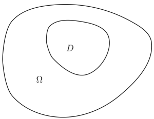
Figure 1: Setting of the paper: Domain $\Omega\subset{\mathbb{R}}^{d}$ that contains the closure of domain $D$. In the set $\Omega\setminus\overline{D}$ the material parameters approach negative value and are positive outside this set.

We will also consider the equations (1.1)-(1.3) in divergence form. To this end, we define a piecewise constant function $a_{\eta}$ by

$$a_{\eta}(x)=a_{\text{e}}>0\text{ in }D\text{ and }\mathbb{R}^{2}\setminus\overline{\Omega},$$ (1.5)

$$a_{\eta}(x)=a_{\text{i}}=a_{\text{e}}(-1+\eta)\text{ in }\Omega\setminus\overline{D},\quad\eta\in{\mathbb{C}},\ \hbox{Im}\,\eta\geq 0,$$ (1.6)

and

$$\tau_{1}=\tau_{2}=\tau=\frac{a_{\text{e}}}{a_{\text{i}}}=(-1+\eta)^{-1}.$$ (1.7)

Typically, the parameter $\eta$ above will be small and purely imaginary. A weak solution of

$$\nabla\cdot a_{\eta}(x)\nabla u+\omega^{2}(\chi_{D\cup{\mathbb{R}}^{d}\setminus\overline{\Omega}}+b\chi_{\Omega\setminus\overline{D}})\mu_{0}u=f\,{\rm in}\,{\mathbb{R}}^{d},\,f\in{\cal E}^{\prime}(\mathbb{R}^{d}\setminus\overline{\Omega}),$$ (1.8)

where $b$ is a complex constant, is obtained from $u_{1}=u|_{D}$, $u_{2}=u|_{\Omega\setminus\overline{\mathbb{D}}}$ and $u_{3}=u|_{{\mathbb{R}}^{d}\setminus\overline{\Omega}}$ solving (1.1)–(1.3), where the transmission coefficients satisfy (1.7). Note that since outside the interfaces $u$ solves a Helmholtz–equation, it has one sided weak normal derivatives on both interfaces. Also, the wave numbers are determined by

$$k_{e}^{2}=\omega^{2}\mu_{0}a_{\text{e}}^{-1},\,k_{i}^{2}=k_{i}(\eta)^{2}:=\omega^{2}\mu_{0}a_{\text{i}}^{-1}b,$$

and depending on our choice of $b$ and $\eta$ the sign of $\hbox{Re}\,k_{i}^{2}$ may vary. We will in particular consider two physically interesting cases. In the first case, $b=1$, and $\hbox{Re}\,k_{i}^{2}\leq 0$. In the second case, $b=-1$ and $\hbox{Re}\,k_{i}^{2}\geq 0$. For more on the physical relevance of these cases, please see the Appendix at end of the article. We also denote

$$k_{i,0}^{2}=k_{i}(\eta)^{2}|_{\eta=0}=-\omega^{2}\mu_{0}a_{\text{e}}^{-1}b.$$ (1.9)

We are especially interested in the behavior of the solutions – and of course in the unique solvability – as $\eta\to 0$ when the ellipticity of (1.1)–(1) degenerates. Physically this corresponds to having a layer of (meta)material in $\Omega\setminus\overline{D}$. More precisely, as explained in the Appendix, in ${\mathbb{R}}^{2}$ this problem comes up when considering time-harmonic TE-polarized waves in the cylinder $\mathbb{R}^{2}\times\mathbb{R}$ with the dielectric constants given by a piecewise constant $a_{\eta}^{-1}$.

It is known that in the case when $\Omega=B(0,R_{1})$ and $D=B(0,1)$ are discs (see [2, 3, 22, 23]) and $\omega=0$ that when $\eta\to 0$ there is a limit radius $R^{*}>0$ s.t. if

$$\hbox{supp}\,(f)\subset(\mathbb{R}^{2}\setminus\overline{\Omega})\cap\{x;|x|>R^{*}\}$$

the solution of (1.1)–(1) will have a bounded $H^{1}$-norm in $\Omega\setminus\overline{D}$ as $\eta\to 0$, but when

$$\hbox{supp}\,(f)\subset(\mathbb{R}^{2}\setminus\overline{\Omega})\cap B(0,R^{*})$$

the $H^{1}(\Omega\setminus\overline{D})$–norm of $u_{2}$ blows up at least as ${\cal O}(|\eta|^{-1/2})$. This phenomenon is called anomalous localized resonance (ALR). To clarify the results of this paper, we make the following formal definitions:

Definition 1.1.

Let $v_{i}^{\eta}$, $i=1,2,3$, be the unique solutions of (1.1)–(1) for $\eta\not=0$ with a given, fixed source term $f\in{\cal E}^{\prime}({\mathbb{R}}^{d}\setminus\overline{\Omega})$.

1. If $\limsup_{\eta\to 0}\|v_{2}^{\eta}\|_{H^{1}(\Omega\setminus\overline{D})}=\infty$, we say that the Weak Anomalous Localized Resonanace (w-ALR) occurs.

2. If $\|v_{2}^{\eta}\|_{H^{1}(\Omega\setminus\overline{D})}\geq C/|\eta|^{1/2}$ as $\eta\to 0$, we say that the Anomalous Localized Resonanace (ALR) occurs.

In this paper we show that neither ALR nor w-ALR happens in $\mathbb{R}^{d}$, $d\geq 3$, when the boundaries of $\Omega$ and $D$ are strictly convex as embedded hypersurfaces of ${\mathbb{R}}^{d}$. We also prove that if the exterior boundary has a flat part then w-ALR will occur even without the quasi-static approximation. Numerical simulations explained in the Appendix support the hypothesis that w-ALR is a weaker phenomenon than ALR. Note, that in [2] the authors define a condition called weak-CALR. In our case this is equivalent to having

$$\limsup_{\eta\to 0}|\eta|^{1/2}\|v_{2}^{\eta}\|_{H^{1}(\Omega\setminus\overline{D})}=\infty$$

and hence is stronger than w-ALR.

In the seminal papers by Milton et al [22, 23] it was observed that ALR happens in the two-dimensional case when $\Omega$ and $D$ are co-centric disc, i.e., $\Omega\setminus\overline{D}$ is an annulus, in the quasi-static regime. This case corresponds to a “perfect lens” made of negative material with a small conductivity $|\eta|$ when $|\eta|\to 0$. When this device is located in a homogeneous electric field and a polarizable point-like object is taken close to the object, the point-like object produces a point source due to the background field. When the object is sufficiently close to the annulus, the induced fields in the annulus blow up as $|\eta|\to 0$. Surprisingly, the fields in the annulus create a field which far away cancels the field produced by the point like-object. This result can be interpreted by saying that the annulus makes the point-like object invisible. Presently, this phenomena is called “exterior cloaking”. It is closely related to other type of invisibility cloaking techniques, the transformation optics based cloaking, see [10, 11, 12, 13, 14, 15, 20, 19, 28] and active cloaking, see [33, 34]. These cloaking examples can be considered as counterexamples for unique solvability of various inverse problems that show the limitations of various imaging modalities. [35, 36].

Results of Milton et al [22, 23] raised plenty of interest and motivated many studies on the topic. The cloaking due to anomalous localized resonance is studied in the quasi-static regime for a general domain in [2]. There, it is shown that in ${\mathbb{R}}^{2}$ the resonance happens for a large class of the sources and that the resonance occurs not because of system approaching an eigenstate, but because of the divergence of an infinite sum of terms related to spectral decomposition of the Neumann-Poincare operator. In [18] the ALR is studied in the quasi-static regime in the two dimensional case when the outer domain $\Omega$ is a disc and the core $D$ is an arbitrary domain compactly supported in $\Omega.$ ALR in the case of confocal ellipses is studied in [6].

In [3], it was shown that the cloaking due to anomalous localized resonance does not happen in ${\mathbb{R}}^{3}$ when $\Omega$ and $D$ are co-centric balls. In [4], cloaking due to anomalous localized resonance is connected to transformation optics and there it is shown that ALR may happen in three dimensional case when the coefficients of the equations are appropriately chosen matrix-valued functions, i.e. correspond to the non-homogeneous anisotropic material.

Earlier, ALR has been studied without the quasi-static approximation both in the 2 and 3 dimensional cases in [25, 26]. In these papers the appearance of ALR is connected to the compatibility of the sources. The compatibility means that for these sources there exists solutions for certain non-elliptic boundary value problems, that are analogous to the so-called interior transmission problems.

In this paper we show that w-ALR either happens or does not happen when certain simple geometric conditions hold: We show that w-ALR - and hence also ALR - do not happen in 3 and higher dimensional case when the boundaries $\partial\Omega$ and $\partial D$ are strictly convex, and also show that w-ALR does happen in $d$-dimensional case, $d\geq 2$ with some sources when the boundary of $\partial\Omega$ contains a flat part. These results show that w-ALR is directly related to geometric properties of the boundaries, and that the behavior of the solutions of the Helmholtz equation with a positive frequency is very different to the solutions in the quasi-static regime.

The first main result deals with the solvablity of the case $\tau_{1}=\tau_{2}=\tau=-1$ when the ellipticity of the transmission problem degenerates. Below we will use the notation $\overline{H}^{1}_{\text{loc}}(\mathbb{R}^{d}\setminus\overline{\Omega})=\{u;\,u=w|_{{\mathbb{R}}^{3}\setminus\overline{\Omega}},\,w\in H^{1}_{\rm loc}({\mathbb{R}}^{d})\}$. Also, we assume in both Theorems below that the following injectivity assumption is valid:

• Injectivity assumption (A): Assume that the equation (1.1)–(1) has only the trivial solution $v_{1}=v_{2}=v_{3}=0$ when $f=0$.

The first main result shows that under certain geometric conditions on the boundary interfaces the limit problem $\eta=0$ is solvable.

Theorem 1.2.

Let $d\geq 3$. Assume that the interior boundary $\Gamma_{1}$ and the exterior boundary $\Gamma_{2}$ are smooth and strictly convex. Assume also that $\eta=0$, so that $\tau=-1$, and that $k_{\text{e}}>0$, $k_{i,0}^{2}$ is not a Dirichlet eigenvalue of $-\Delta$ in $D$ and ${\mathbb{R}}^{d}\setminus\overline{\Omega}$, and $k_{e}^{2}$ is not a Dirichlet eigenvalue of $-\Delta$ in $\Omega$. Then given $K\subset\mathbb{R}^{d}\setminus\overline{\Omega}$ compact and $f\in H^{s}(\mathbb{R}^{d}\setminus\overline{\Omega})$ with $\hbox{supp}\,(f)\subset K$, the problem (1.1)–(1) has a unique solution $v_{1}\in H^{1}(D)$, $v_{2}\in H^{1}(\Omega\setminus D)$ and $v_{3}\in\overline{H}^{1}_{\text{loc}}(\mathbb{R}^{d}\setminus\overline{\Omega})$ such

$$\left\|v_{2}\right\|_{H^{1}(\Omega\setminus\overline{D})}\leq C_{K}\left\|f\right\|_{H^{s}(\mathbb{R}^{d}\setminus\overline{\Omega})}.$$

We can also prove the following limiting result when $\eta\to 0$.

Theorem 1.3.

Let $d\geq 3$. Assume that the interfaces $\Gamma_{1}$ and $\Gamma_{2}$ are smooth and strictly convex and let $f$ be as in the previous Theorem. Let $\tau=\tau(\eta)=(-1+\eta)^{-1}$, $\eta\in{\mathbb{C}}$. Assume also that $k_{\text{e}}>0$, $k_{i,0}^{2}$ is not a Dirichlet eigenvalue of $-\Delta$ in $D$, and $k_{e}^{2}$ is not a Dirichlet eigenvalue of $-\Delta$ in $\Omega$. Then the problem (1.1)–(1) with $\tau=\tau(\eta)$ is uniquely solvable for $|\eta|$ small enough, and if $v_{i}^{\eta}$, $i=1,2,3$ are its solutions and $v_{i}$, $i=1,2,3$ the solutions given by Theorem 1.2, we have as $\eta\to 0$ in a complement of a open conical neighborhood of $i{\mathbb{R}}$,

$$v_{1}^{\eta}\xrightarrow[H^{1}(D)]{}v_{1},\quad v_{2}^{\eta}\xrightarrow[H^{1}(\Omega\setminus\overline{D})]{}v_{2},\quad v_{3}^{\eta}\xrightarrow[\overline{H}_{\text{loc}}^{1}(\mathbb{R}^{d}\setminus\overline{\Omega})]{}v_{3}.$$

Both of these theorems will be proven in section four of this paper.

Some comments are in order. First of all, under the assumptions of the above theorems, given a fixed source distribution $f$ supported in ${\mathbb{R}}^{d}\setminus\overline{\Omega}$, the solution $v_{2}^{\eta}$ tends to a $H^{1}$–function $v_{2}$ as $\eta\to 0$, and thus there is no blow up.

Secondly, in Proposition 4.1 we give sufficient conditions for the injectivity assumption (A) to hold. Especially, if the wave numbers come from a divergence type equation with piecewise constant coefficients, so that (1.5) – (1.7) are valid, the injctivity will hold.

Finally, the remaining conditions assumed of the wavenumbers are related to the boundary integral equation we use, and quarantee the equivalence of it with the original transmission problem. We believe that using another reduction to the boundary these could be relaxed.

2 Layer potentials

As a first step we are going to reduce (1.1)–(1) to an equivalent problem on the boundary interfaces. The first step it to replace the source $f$ with equivalent boundary currents. So, fix $f\in H^{s}_{0}(\mathbb{R}^{d}\setminus\overline{\Omega})$ and let $v$ be the unique solution of the problem

$$-(\Delta+k_{e}^{2})v = f\,\,\mbox{in $\mathbb{R}^{d}\setminus\overline{\Omega}$},$$ (2.1)

$$v|_{\Gamma_{2}} = 0$$ (2.2)

that satisfies the Sommerfeld radiation condition (1). Then, if we let $\widetilde{v}_{3}=v_{3}-v$ in (1.1)–(1) we see that $v_{1},\,v_{2}$ and $\widetilde{v}_{3}$ will satisfy the transmission problem consisting of equation (1.1) with radiation condition (1) and the transmission conditions

$$v_{1}|_{\Gamma_{1}}=v_{2}|_{\Gamma_{1}},\quad\tau_{1}\partial_{\nu}v_{1}|_{\Gamma_{1}}=\partial_{\nu}v_{2}|_{\Gamma_{1}}$$ (2.3)

and

$$\widetilde{v}_{3}|_{\Gamma_{2}}=v_{2}|_{\Gamma_{2}}-f_{2},\quad\tau_{2}\partial_{\nu}\widetilde{v}_{3}|_{\Gamma_{2}}=\partial_{\nu}v_{2}|_{\Gamma_{2}}-g_{2}$$

where $f_{2}=v|_{\Gamma_{2}}\in H^{1/2}(\Gamma_{2})$ and $g_{2}=\partial_{\nu}v|_{\Gamma_{2}}\in H^{-1/2}(\Gamma_{2})$. Hence, we are going to study first the transmission problem

$$-(\Delta+k_{\text{e}}^{2})u_{1} = 0\text{ in }D$$ (2.4)

$$-(\Delta+k_{\text{i}}^{2})u_{2} = 0\text{ in }\Omega\setminus\overline{D}$$ (2.5)

$$-(\Delta+k_{\text{e}}^{2})\widetilde{u}_{3} = 0\text{ in }\mathbb{R}^{d}\setminus\overline{\Omega}$$ (2.6)

$$u_{1}|_{\Gamma_{1}}=u_{2}|_{\Gamma_{1}}-f_{1},\quad\tau_{1}\partial_{\nu}u_{1}|_{\Gamma_{1}} = \partial_{\nu}u_{2}|_{\Gamma_{1}}-g_{1}$$ (2.7)

$$u_{2}|_{\Gamma_{2}}=u_{3}|_{\Gamma_{2}}-f_{2},\quad\tau_{2}\partial_{\nu}u_{3}|_{\Gamma_{2}} = \partial_{\nu}u_{2}|_{\Gamma_{2}}-g_{2}$$ (2.8)

$$u_{3}\text{ satisfies Sommerfeld condition (\ref{Sommerfeld}).}$$ (2.9)

where $f_{1}\in H^{s}(\Gamma_{1})$, $g_{1}\in H^{s-1}(\Gamma_{1})$, $f_{2}\in H^{s}(\Gamma_{2})$ and $g_{2}\in H^{s-1}(\Gamma_{2})$ for some real value of $s$. Notice also that since the source $f$ is supported away from $\Gamma_{2}$ the solution $v$ of (2.1) will actually be smooth near $\Gamma_{2}$, and hence the boundary jumps $f_{i}$ and $g_{i}$ will be $C^{\infty}$ functions. This will be crucial for our argument.

The reduction to the boundary will be done in the usual way, i.e. by using suitable layer potential operators. Given $k\in\mathbb{C}$, $\operatorname{\mathrm{Im}}k\geq 0$, let

$$G_{k}(x)=\begin{cases}\frac{i}{4}\left(\frac{k}{2\pi|x|}\right)^{\frac{d-2}{2}}H^{(1)}_{\frac{d-2}{2}}(k|x|),\quad k\neq 0,\quad d\geq 2\\[8.61108pt] \frac{\Gamma\left(\frac{d-2}{2}\right)}{4\pi^{\frac{d}{2}}}|x|^{2-d},\quad k=0,\quad d\geq 3\\[8.61108pt] \frac{1}{2\pi}\ln|x|,\quad d=2,\,k=0.\end{cases}$$

be the fundamental solution of $-(\Delta+k^{2})$ in $\mathbb{R}^{d}$ satisfying Sommerfeld condition (1).

For $\Gamma=\Gamma_{1}$ or $\Gamma=\Gamma_{2}$, we define using these kernels the (volume) single layer operators by

$$S_{k}^{\Gamma}(\phi)(x)=\int_{\Gamma}G_{k}(x-y)\phi(y)\mathrm{d}S(y),\quad x\notin\Gamma,\quad\phi\in C^{\infty}(\Gamma)$$

Sometimes when we wish to emphasize that we are restricting these operators to a domain $\Omega$, $\Gamma\cap\Omega=\emptyset$, we use the notations $S_{k}^{\Gamma,\Omega}(\phi)=S_{k}^{\Gamma}(\phi)|_{\Omega}$. These operators define continuous mappings $S_{k}^{\Gamma}:C^{\infty}(\Gamma)\to D^{\prime}(\mathbb{R}^{d}\setminus\Gamma)$.

Similarly, we define the (volume) double layer operators by

$$D_{k}^{\Gamma}(\phi)(x)=\int_{\Gamma}\frac{\partial G_{k}(x-y)}{\partial\nu(y)}\phi(y)\mathrm{d}S(y),\quad x\notin\Gamma,\quad\phi\in C^{\infty}(\Gamma)$$

where $\nu$ will always denote the exterior unit normal to $\Omega\setminus D$. Like for the single layer potentials, we will occasionally denote the restrictions of these to $\Omega\subset{\mathbb{R}}^{d}\setminus\Gamma$ by $D_{k}^{\Gamma,\Omega}$. Also, $D_{k}^{\Gamma}:C^{\infty}(\Gamma)\to D^{\prime}(\mathbb{R}^{d}\setminus\Gamma)$ continuously.

Mapping properties of these operators between appropriate Sobolev spaces are also well known (see [5], [21] or [29], page 156, Theorem 4): For all $s\in\mathbb{R}$ we have $S_{k}^{\Gamma,\Omega}:H^{s}(\Gamma)\to H^{s+\frac{3}{2}}(\Omega)$ and $D_{k}^{\Gamma,\Omega}:H^{s}(\Gamma)\to H^{s+\frac{1}{2}}(\Omega)$ if $\Omega\subset\mathbb{R}^{d}\setminus\Gamma$ is a bounded domain.

We need traces of these operators on both $\Gamma_{1}$ and $\Gamma_{2}$. Hence, let $\gamma^{+}_{0,j}$ be the trace operator on $\Gamma_{j}$ from the complement of $\Omega\setminus\overline{D}$, that is, $\gamma^{+}_{0,j}(u)=u|_{\Gamma_{j}}$ for $u\in H^{1}(({\mathbb{R}}^{d}\setminus\overline{\Omega})\cup D)$. Respectively let $\gamma^{-}_{0,j}$ be the trace–opearator on $\Gamma_{j}$ from $\Omega\setminus\overline{D}$, that is, $\gamma^{-}_{0,j}(u)=u|_{\Gamma_{j}}$ for $u\in H^{1}(\Omega\setminus\overline{D})$. Then, for $\phi\in H^{s}(\Gamma_{j})$, $s>-1$, we have

$$\gamma^{+}_{0,j}S^{\Gamma_{j}}_{k}\phi=V_{k}^{\Gamma_{j}}\phi=\gamma^{-}_{0,j}S^{\Gamma_{j}}_{k}\phi,$$ (2.10)

where

$$V_{k}^{\Gamma_{j}}\phi(x)=\int_{\Gamma_{j}}G_{k}(x-y)\phi(y)\mathrm{d}S(y)$$ (2.11)

is the trace-single-layer operator on $\Gamma_{j}$.

Also, if $\psi\in H^{s}(\Gamma_{j})$, $s>0$, for the traces of the double layer we have the jump relations

$$\gamma^{-}_{0,j}D_{k}^{\Gamma_{j}}\psi+\frac{\psi}{2}=\gamma^{+}_{0,j}D_{k}^{\Gamma_{j}}\psi-\frac{\psi}{2}=K_{k}^{\Gamma_{j}}\psi,$$ (2.12)

where $K_{k}^{\Gamma_{j}}$ is the trace-double-layer operator on $\Gamma_{j}$ given by

$$K_{k}^{\Gamma}\phi(x)=p.v.\int_{\Gamma_{j}}\frac{\partial G_{k}(x-y)}{\partial\nu(y)}\phi(y)\mathrm{d}S(y).$$ (2.13)

The maps $K_{k}^{\Gamma_{j}}:H^{s}(\Gamma_{j})\to H^{s}(\Gamma_{j})$ and $S_{k}^{\Gamma_{j}}:H^{s}(\Gamma_{j})\to H^{s+1}(\Gamma_{j})$ are continous pseudodifferential operators for any $s\in{\mathbb{R}}$.

Next, let $\gamma^{+}_{1,j}$ be the trace of the normal derivative on $\Gamma_{j}$ from the complement of $\Omega\setminus\overline{D}$, that is, $\gamma^{+}_{1,j}(u)=\partial_{\nu}u|_{\Gamma_{j}}$ for $u\in H^{1}(({\mathbb{R}}^{d}\setminus\overline{\Omega})\cup D)$. Respectively let $\gamma^{-}_{1,j}$ be the trace of the normal derivative on $\Gamma_{j}$ from $\Omega\setminus\overline{D}$, that is, $\gamma^{-}_{1,j}(u)=\partial_{\nu}u|_{\Gamma_{j}}$ for $u\in H^{1}(\Omega\setminus\overline{D})$. . For the normal derivatives of the single layer potentials we have the jump relations

$$\gamma^{-}_{1,j}S_{k}^{\Gamma_{j}}\phi-\frac{\phi}{2}=\gamma^{+}_{1,j}S_{k}^{\Gamma_{j}}\phi+\frac{\phi}{2}=K_{k}^{*,\Gamma_{j}}\phi,$$ (2.14)

for any $\phi\in H^{-1/2}(\Gamma_{j})$, where the operator $K_{k}^{*,\Gamma_{j}}$ is the adjoint trace-double-layer operator on $\Gamma_{j}$ given by

$$K_{k}^{*,\Gamma_{j}}\phi(x)=p.v.\int_{\Gamma_{j}}\frac{\partial G_{k}(x-y)}{\partial\nu(x)}\phi(y)\mathrm{d}S(y),$$ (2.15)

For $H^{1}$–solutions of an inhomogeneous Helmholz–equation with an $L^{2}$–source one can define normal traces weakly using Green’s theorems. With this interpretation, for any $\psi\in H^{1/2}(\Gamma_{j})$, we also have the traces

$$\gamma^{-}_{1,j}D_{k}^{\Gamma_{j}}\psi=\gamma^{+}_{1,j}D_{k}^{\Gamma_{j}}\psi=N_{k}^{\Gamma_{j}}\psi,$$ (2.16)

where the hypersingular integral operator $N_{k}^{\Gamma_{j}}$ has (formally) the kernel

$$\frac{\partial^{2}G_{k}(x-y)}{\partial\nu(x)\partial\nu(y)},\,\,x,\,y\in\Gamma_{j},\,x\not=y.$$

The maps $K_{k}^{*,\Gamma_{j}}:H^{s}(\Gamma_{j})\to H^{s}(\Gamma_{j})$ and $N_{k}^{\Gamma_{j}}:H^{s}(\Gamma_{j})\to H^{s-1}(\Gamma_{j})$ are continous pseudodifferential operators for any $s\in{\mathbb{R}}$.

3 Reduction to the boundary

We will follow the ideas of [17] adapted to our situation, where we have two interfaces instead of just one. Let us consider (2.4)–(2.9). Write an ansaz for $u_{1}$ and $u_{3}$:

$$u_{1}=S_{{k_{\text{e}}}}^{{\Gamma_{1},D}}(\phi),\quad\phi\in H^{-\frac{1}{2}}(\Gamma_{1}),$$ (3.1)

$$u_{3}=S_{{k_{\text{e}}}}^{{\Gamma_{2},\mathbb{R}^{d}\setminus\overline{\Omega}}}(\psi),\quad\psi\in H^{-\frac{1}{2}}(\Gamma_{2}),$$ (3.2)

and to

$$u_{2}\in{\cal L}:=\{v\in H^{1}(\Omega\setminus\overline{D});\ -(\Delta+k_{\text{i}}^{2})v=0\}$$

we apply the representation theorem (see for example [7]) to get

$$u_{2} = S_{{k_{\text{i}}{}}}^{{\Gamma_{1},\Omega\setminus\overline{D}}}\left(\left.\frac{\partial u_{2}}{\partial\nu}\right|_{\Gamma_{1}}\right)-D_{{k_{\text{i}}{}}}^{{\Gamma_{1},\Omega\setminus\overline{D}}}\left(u_{2}|_{\Gamma_{1}}\right)$$

$$+S_{{k_{\text{i}}{}}}^{{\Gamma_{2},\Omega\setminus\overline{D}}}\left(\left.\frac{\partial u_{2}}{\partial\nu}\right|_{\Gamma_{2}}\right)-D_{{k_{\text{i}}{}}}^{{\Gamma_{1},\Omega\setminus\overline{D}}}\left(u_{2}|_{\Gamma_{2}}\right),\text{ in }\Omega\setminus\overline{D}.$$

Taking traces from $D$ on $\Gamma_{1}$ we get

$$\gamma^{+}_{0,1}u_{1}=V_{{k_{\text{e}}}}^{{\Gamma_{1}}}(\phi),\quad\gamma^{+}_{1,1}u_{1}=K_{{k_{\text{e}}}}^{{*,\Gamma_{1}}}(\phi)-\frac{\phi}{2},$$ (3.4)

and taking traces from $\mathbb{R}^{d}\setminus\overline{\Omega}$ on $\Gamma_{2}$ we get

$$\gamma^{+}_{0,2}u_{3}=V_{{k_{\text{e}}}}^{{\Gamma_{2}}}(\psi),\quad\gamma^{+}_{1,2}u_{3}=K_{{k_{\text{e}}}}^{{*,\Gamma_{2}}}(\psi)-\frac{\psi}{2}.$$ (3.5)

Now, denote

$$A_{i}f =\left.S_{{k_{\text{i}}{}}}^{{\Gamma_{j},\Omega\setminus\overline{D}}}(f)\right|_{\Gamma_{i}},\quad i\neq j,\quad f\in H^{-\frac{1}{2}}(\Gamma_{j})$$

$$B_{i}f =\left.\frac{\partial S_{{k_{\text{i}}{}}}^{{\Gamma_{j},\Omega\setminus\overline{D}}}(f)}{\partial\nu}\right|_{\Gamma_{i}},\quad i\neq j,\quad f\in H^{-\frac{1}{2}}(\Gamma_{j})$$

$$R_{i}g =\left.D_{{k_{\text{i}}{}}}^{{\Gamma_{j},\Omega\setminus\overline{D}}}(g)\right|_{\Gamma_{i}},\quad i\neq j,\quad g\in H^{\frac{1}{2}}(\Gamma_{j})$$

$$S_{i}g =\left.\frac{\partial D_{{k_{\text{i}}{}}}^{{\Gamma_{j},\Omega\setminus\overline{D}}}(g)}{\partial\nu}\right|_{\Gamma_{i}},\quad i\neq j,\quad g\in H^{\frac{1}{2}}(\Gamma_{j}).$$

Note that all these operators have $C^{\infty}$–smooth kernels. Taking traces of $u_{2}$ on $\Gamma_{1}$ and $\Gamma_{2}$ we get

$$\gamma^{-}_{0,1}u_{2} =V_{{k_{\text{i}}{}}}^{{\Gamma_{1}}}\left(\partial_{\nu}u_{2}|_{\Gamma_{1}}\right)-K_{{k_{\text{i}}{}}}^{{\Gamma_{1}}}\left(u_{2}|_{\Gamma_{1}}\right)+\left.\frac{u_{2}}{2}\right|_{\Gamma_{1}}+A_{1}\left(\partial_{\nu}u_{2}|_{\Gamma_{2}}\right)-R_{1}(u_{2}|_{\Gamma_{2}})$$ (3.6)

$$\gamma^{-}_{0,2}u_{2} =V_{{k_{\text{i}}{}}}^{{\Gamma_{2}}}\left(\partial_{\nu}u_{2}|_{\Gamma_{2}}\right)-K_{{k_{\text{i}}{}}}^{{\Gamma_{2}}}\left(u_{2}|_{\Gamma_{2}}\right)+\left.\frac{u_{2}}{2}\right|_{\Gamma_{2}}+A_{2}\left(\partial_{\nu}u_{2}|_{\Gamma_{1}}\right)-R_{2}(u_{2}|_{\Gamma_{1}})$$ (3.7)

and for the traces of the normal derivatives we get

$$\gamma^{-}_{1,1}u_{2}=K_{{k_{\text{i}}{}}}^{{*,\Gamma_{1}}}(\partial_{\nu}u_{2}|_{\Gamma_{1}})+\left.\frac{\partial_{\nu}u_{2}}{2}\right|_{\Gamma_{1}}-N_{{k_{\text{i}}{}}}^{{\Gamma_{1}}}(u_{2}|_{\Gamma_{1}})+B_{1}\left(\partial_{\nu}u_{2}|_{\Gamma_{2}}\right)-S_{1}(u_{2}|_{\Gamma_{2}})$$

and

$$\gamma^{-}_{1,2}u_{2}=K_{{k_{\text{i}}{}}}^{{*,\Gamma_{2}}}(\partial_{\nu}u_{2}|_{\Gamma_{2}})+\left.\frac{\partial_{\nu}u_{2}}{2}\right|_{\Gamma_{2}}-N_{{k_{\text{i}}{}}}^{{\Gamma_{2}}}(u_{2}|_{\Gamma_{2}})+B_{2}\left(\partial_{\nu}u_{2}|_{\Gamma_{1}}\right)-S_{2}(u_{2}|_{\Gamma_{1}}).$$

Recall next the transmission conditions

$$u_{1}|_{\Gamma_{1}} =u_{2}|_{\Gamma_{1}}-f_{1},\quad\tau_{1}\partial_{\nu}u_{1}|_{\Gamma_{1}}=\partial_{\nu}u_{2}|_{\Gamma_{1}}-g_{1},$$ (3.8)

$$u_{3}|_{\Gamma_{2}} =u_{2}|_{\Gamma_{2}}-f_{2},\quad\tau_{2}\partial_{\nu}u_{3}|_{\Gamma_{2}}=\partial_{\nu}u_{2}|_{\Gamma_{2}}-g_{2},$$ (3.9)

$$f_{i}\in H^{\frac{1}{2}}(\Gamma_{i}),\quad g_{i}\in H^{-\frac{1}{2}}(\Gamma_{i})$$

If one substitutes (3.8) to (3.6) one gets an integral equation

$$\frac{\gamma^{+}_{0,1}u_{1}}{2}+K_{{k_{\text{i}}{}}}^{{\Gamma_{1}}}(\gamma^{+}_{0,1}u_{1})-\tau_{1}V_{{k_{\text{i}}{}}}^{{\Gamma_{1}}}(\gamma^{+}_{1,1}u_{1})+\tau_{2}A_{1}(\gamma^{+}_{1,2}u_{3})-R_{1}(\gamma^{+}_{0,2}u_{3})=\widetilde{f}_{1}$$

where

$$\widetilde{f}_{1}:=-\frac{f_{1}}{2}+V_{{k_{\text{i}}{}}}^{{\Gamma_{1}}}(g_{1})-K_{{k_{\text{i}}{}}}^{{\Gamma_{1}}}(f_{1})+A_{1}(g_{2})-R_{1}(f_{2}).$$ (3.10)

Next, using (3.4) and (3.5) we write the boundary values of $u_{1}$ and $u_{3}$ in terms of $\psi$ and $\phi$. This gives an boundary integral equation on $\Gamma_{1}$:

$$\frac{1}{2}\left(V_{{k_{\text{e}}}}^{{\Gamma_{1}}}+\tau_{1}V_{{k_{\text{i}}{}}}^{{\Gamma_{1}}}\right)(\phi)+\left(K_{{k_{\text{i}}{}}}^{{\Gamma_{1}}}V_{{k_{\text{e}}}}^{{\Gamma_{1}}}-\tau_{1}V_{{k_{\text{i}}{}}}^{{\Gamma_{1}}}K_{{k_{\text{e}}}}^{{*,\Gamma_{1}}}\right)(\phi)+M_{1}(\psi)=\widetilde{f}_{1},$$ (3.11)

where

$$M_{1}(\psi)=\tau_{2}A_{1}K_{{k_{\text{e}}}}^{{*,\Gamma_{2}}}(\psi)-\frac{\tau_{2}}{2}A_{1}(\psi)-R_{1}V_{{k_{\text{e}}}}^{{\Gamma_{2}}}(\psi)$$

is a smoothing operator. Substituting similarly (3.9) to (3.7) one gets an boundary integral equation on $\Gamma_{2}$:

$$\frac{1}{2}\left(V_{{k_{\text{e}}}}^{{\Gamma_{2}}}+\tau_{2}V_{{k_{\text{i}}{}}}^{{\Gamma_{2}}}\right)(\psi)+\left(K_{{k_{\text{i}}{}}}^{{\Gamma_{2}}}V_{{k_{\text{e}}}}^{{\Gamma_{1}}}-\tau_{2}V_{{k_{\text{i}}{}}}^{{\Gamma_{2}}}K_{{k_{\text{e}}}}^{{*,\Gamma_{2}}}\right)(\psi)+M_{2}(\phi)=\widetilde{f}_{2},$$ (3.12)

where

$$M_{2}(\phi)=\frac{\tau_{2}}{2}A_{2}(\phi)-\tau_{2}A_{2}K_{{k_{\text{e}}}}^{{*,\Gamma_{1}}}(\phi)+R_{2}V_{{k_{\text{e}}}}^{{\Gamma_{1}}}(\phi)$$

is smoothing and

$$\widetilde{f}_{2}:=-\frac{f_{2}}{2}+V_{{k_{\text{i}}{}}}^{{\Gamma_{2}}}(g_{2})-K_{{k_{\text{i}}{}}}^{{\Gamma_{2}}}(f_{2})+A_{2}(g_{1})-R_{2}(f_{1}).$$ (3.13)

We combine the two equations above as follows: for $(\phi,\psi)\in H^{-\frac{1}{2}}(\Gamma_{1})\times H^{-\frac{1}{2}}(\Gamma_{2})$ we have

$$(\mathcal{A}+\mathcal{M})\begin{pmatrix}\phi\\ \psi\end{pmatrix}=\widetilde{f}:=\begin{pmatrix}\widetilde{f}_{1}\\ \widetilde{f}_{2}\end{pmatrix}$$ (3.14)

where

$$\mathcal{A} = \begin{pmatrix}\mathcal{A}_{1}&0\\ 0&\mathcal{A}_{2}\end{pmatrix},$$ (3.15)

$$\mathcal{M} = \begin{pmatrix}0&M_{1}\\ M_{2}&0\end{pmatrix}$$

and

$$\mathcal{A}_{1} =\frac{1}{2}\left(V_{{k_{\text{e}}}}^{{\Gamma_{1}}}+\tau_{1}V_{{k_{\text{i}}{}}}^{{\Gamma_{1}}}\right)+\left(K_{{k_{\text{i}}{}}}^{{\Gamma_{1}}}V_{{k_{\text{e}}}}^{{\Gamma_{1}}}-\tau_{1}V_{{k_{\text{i}}{}}}^{{\Gamma_{1}}}K_{{k_{\text{e}}}}^{{*,\Gamma_{1}}}\right),$$

$$\mathcal{A}_{2} =\frac{1}{2}\left(V_{{k_{\text{e}}}}^{{\Gamma_{2}}}+\tau_{2}V_{{k_{\text{i}}{}}}^{{\Gamma_{2}}}\right)+\left(K_{{k_{\text{i}}{}}}^{{\Gamma_{2}}}V_{{k_{\text{e}}}}^{{\Gamma_{1}}}-\tau_{2}V_{{k_{\text{i}}{}}}^{{\Gamma_{2}}}K_{{k_{\text{e}}}}^{{*,\Gamma_{2}}}\right).$$

This is the integral equation we are going to study.

The next proposition establishes conditions under which (3.14) is equivalent with the original transmission problem (2.4)–(2.9).

Proposition 3.1.

Assume $k_{\text{i}}^{2}$ is not an Dirichlet eigenvalue of $-\Delta$ in $D$ or in ${\mathbb{R}}^{3}\setminus{\overline{\Omega}}$ . If $u_{1}\in H^{1}(D)$, $u_{2}\in H^{1}(\Omega\setminus\overline{D})$ and $u_{3}\in\overline{H}^{1}_{\text{loc}}(\mathbb{R}^{d}\setminus\overline{\Omega})$ solve (2.4)–(2.9), then $\phi\in H^{{-\frac{1}{2}}}({\Gamma_{1}})$, $\psi\in H^{{-\frac{1}{2}}}({\Gamma_{2}})$ satisfying (3.1)–(3.2) solve (3.14).

Conversely, assume that $(\phi,\psi)\in H^{{-\frac{1}{2}}}({\Gamma_{1}})\times H^{{-\frac{1}{2}}}({\Gamma_{2}})$ solve (3.14). Define $u_{1}$ and $u_{3}$ by (3.1)–(3.2) and $u_{2}$ by

$$u_{2} = S_{{k_{\text{i}}{}}}^{{\Gamma_{1}}}\left(\tau_{1}\left[K_{{k_{\text{e}}}}^{{*,\Gamma_{1}}}(\phi)-\frac{\phi}{2}\right]+g_{1}\right)-D_{{k_{\text{i}}{}}}^{{\Gamma_{1}}}\left(V_{{k_{\text{e}}}}^{{\Gamma_{1}}}(\phi)+f_{1}\right)$$

$$\phantom{=}+S_{{k_{\text{i}}{}}}^{{\Gamma_{2}}}\left(\tau_{2}\left[K_{{k_{\text{e}}}}^{{*,\Gamma_{2}}}(\psi)-\frac{\psi}{2}\right]+g_{2}\right)-D_{{k_{\text{i}}{}}}^{{\Gamma_{2}}}\left(V_{{k_{\text{e}}}}^{{\Gamma_{2}}}(\psi)+f_{2}\right).$$

Then the triplet $(u_{1},u_{2},u_{3})\in H^{{1}}({D})\times H^{{1}}({\Omega\setminus\overline{D}})\times\overline{H}^{1}_{\text{loc}}(\mathbb{R}^{d}\setminus\overline{\Omega})$ will solve (2.4)–(2.9).

Proof.

It only remains to prove the second claim. So define $u_{2}$ by (3.1) and $u_{1}$ and $u_{3}$ by (3.1)–(3.2) where $\phi\in H^{{-\frac{1}{2}}}({\Gamma_{1}})$, $\psi\in H^{{-\frac{1}{2}}}({\Gamma_{2}})$ solve (3.14). By taking traces on $\Gamma_{1}$ and $\Gamma_{2}$ we immediately recover the transimission conditions

$$u_{1}|_{\Gamma_{1}}=u_{2}|_{\Gamma_{1}}-f_{1},u_{3}|_{\Gamma_{2}}=u_{2}|_{\Gamma_{2}}-f_{2}.$$

To prove the transmission conditions for the normal derivatives we define for $x\in D\cup\mathbb{R}^{d}\setminus\overline{\Omega}$,

$$v(x) = S_{{k_{\text{i}}{}}}^{{\Gamma_{1}}}\left(\tau_{1}\left[K_{{k_{\text{e}}}}^{{*,\Gamma_{1}}}(\phi)-\frac{\phi}{2}\right]+g_{1}\right)(x)-D_{{k_{\text{i}}{}}}^{{\Gamma_{1}}}\left(V_{{k_{\text{e}}}}^{{\Gamma_{1}}}(\phi)+f_{1}\right)(x)$$

$$\phantom{=}+S_{{k_{\text{i}}{}}}^{{\Gamma_{2}}}\left(\tau_{2}\left[K_{{k_{\text{e}}}}^{{*,\Gamma_{2}}}(\psi)-\frac{\psi}{2}\right]+g_{2}\right)(x)-D_{{k_{\text{i}}{}}}^{{\Gamma_{2}}}\left(V_{{k_{\text{e}}}}^{{\Gamma_{2}}}(\psi)+f_{2}\right)(x).$$

Then using (3.14) we see that $v$ solves

$$\begin{cases}(\Delta+k_{\text{i}}^{2})v=0\text{ in }D\\ v|_{\Gamma_{1}}=0\end{cases}$$

and since we assumed that $k_{i}^{2}$ was not an Dirichlet eigenvalue of $-\Delta$ in $D$, we get that $v=0$ in $D$. Similarily the restriction of $v$ to ${\mathbb{R}}^{3}\setminus{\overline{\Omega}}$ is a solution of

$$\begin{cases}-(\Delta+k_{\text{i}}^{2})v=0\text{ in }\mathbb{R}^{d}\setminus\overline{\Omega}\\ v|_{{\partial\Omega}}=0\end{cases}$$

satisfying Sommerfeld condition (1). Hence by the assumptions, $v=0$ also in ${\mathbb{R}}^{3}\setminus{\overline{\Omega}}$. Taking traces of the normal derivative of $v$ from $D$ we get

$$0 = \gamma^{+}_{1,1}v=K_{{k_{\text{i}}{}}}^{{*,\Gamma_{1}}}\left(\tau_{1}\left[K_{{k_{\text{e}}}}^{{*,\Gamma_{1}}}(\phi)-\frac{\phi}{2}\right]+g_{1}\right)$$

$$\phantom{=}-\frac{1}{2}\left(\tau_{1}\left[K_{{k_{\text{e}}}}^{{*,\Gamma_{1}}}(\phi)-\frac{\phi}{2}\right]+g_{1}\right)-N_{{k_{\text{i}}{}}}^{{\Gamma_{1}}}\left(V_{{k_{\text{e}}}}^{{\Gamma_{1}}}(\phi)+f_{1}\right)$$

$$\phantom{=}+B_{1}\left(\tau_{2}\left[K_{{k_{\text{e}}}}^{{*,\Gamma_{2}}}(\psi)-\frac{\psi}{2}\right]+g_{2}\right)-S_{1}\left(V_{{k_{\text{e}}}}^{{\Gamma_{2}}}(\psi)+f_{2}\right),$$

or equivalently,

$$\tau_{1}\left[K_{{k_{\text{e}}}}^{{*,\Gamma_{1}}}(\phi)-\frac{\phi}{2}\right]+g_{1} = K_{{k_{\text{i}}{}}}^{{*,\Gamma_{1}}}\left(\tau_{1}\left[K_{{k_{\text{e}}}}^{{*,\Gamma_{1}}}(\phi)-\frac{\phi}{2}\right]+g_{1}\right)$$

$$\phantom{=}+\frac{1}{2}\left(\tau_{1}\left[K_{{k_{\text{e}}}}^{{*,\Gamma_{1}}}(\phi)-\frac{\phi}{2}\right]+g_{1}\right)-N_{{k_{\text{i}}{}}}^{{\Gamma_{1}}}\left(V_{{k_{\text{i}}{}}}^{{\Gamma_{1}}}(\phi)+f_{1}\right)$$

$$\phantom{=}+B_{1}\left(\tau_{2}\left[K_{{k_{\text{e}}}}^{{*,\Gamma_{2}}}(\psi)-\frac{\psi}{2}\right]+g_{2}\right)-S_{1}\left(V_{{k_{\text{e}}}}^{{\Gamma_{2}}}(\psi)+f_{2}\right).$$

The left-hand side of (3) is $\tau_{1}\partial_{\nu}u_{1}+g_{1}$. The right-hand side is equal to $\partial_{\nu}u_{2}|_{\Gamma_{1}}$. Hence we have shown the second equation in (3.8). Proceeding similarly, but taking traces of $v$ from ${\mathbb{R}}^{3}\setminus{\overline{\Omega}}$, we get the second equation of (3.9). $\square$

Remark 3.2.

Note that the Dirichlet-spectrum of $-\Delta$ on $D$ is discrete and positive, so that always, if $k_{\text{i}}^{2}\leq 0$ or if $\operatorname{\mathrm{Im}}k_{\text{i}}^{2}\not=0$, we have the first condition. Similarly, $\operatorname{\mathrm{Im}}k_{\text{i}}\geq 0$, $k_{\text{i}}\not=0$, is enough to guarantee that the second assumption of Proposition  3.1 is valid. In the case of most interest to us we have $k_{\text{e}}^{2}=\omega^{2}a_{\text{e}}\mu_{0}>0$ and $k_{i}^{2}=\omega^{2}a_{\text{i}}\mu_{0}$ with $a_{\text{i}}=a_{\text{e}}(-1+\eta)$, where $a_{\text{e}}$ and and imaginary part of $\eta$ are positive. Hence the assumptions of Proposition  3.1 are valid.

4 Absence of ALR

As the first step in proving the solvability and stability when $\eta\to 0$ we give a standard uniqueness result (see [8]):

Proposition 4.1.

Assume $k_{\text{e}}>0$, $\operatorname{\mathrm{Re}}\left(k_{\text{i}}^{2}/\tau_{2}\right)\geq 0$ and $\operatorname{\mathrm{Re}}\tau_{1}\tau_{2}^{-1}k_{\text{e}}^{2}\geq 0$. Then the problem (1.1)–(1) has at most one solution. Also, if the wave numbers are associated to a divergence type equation, i.e. (1.5) – (1.7) are satisfied with a real valued parameter $b$, the uniqueness holds.

Proof.

Let $R>0$ be so large that $\overline{\Omega}\subset B_{R}(0)$. Then the Sommerfeld Radiation Condition implies

$$\int_{|x|=R}\partial_{r}u_{3}\cdot\overline{u}_{3}\mathrm{d}S=ik_{e}\lim_{R\to\infty}\int_{|x|=R}|u_{3}|^{2}\,\mathrm{d}S+o(1)\quad\text{as}\,R\to\infty.$$ (4.1)

Now using Green’s formula

$$\int_{|x|=R}\partial_{r}u_{3}\cdot\overline{u}_{3}\mathrm{d}S-\int_{\partial\Omega}\partial_{\nu}u_{3}\cdot\overline{u}_{3}\mathrm{d}S$$

$$=\int_{B_{R}(0)\setminus\overline{\Omega}}\Delta u_{3}\cdot\overline{u}_{3}\mathrm{d}x=\int_{B_{R}(0)\setminus\overline{\Omega}}-k_{\text{e}}^{2}|u_{3}|^{2}\mathrm{d}x,$$

i.e.

$$\int_{|x|=R}\partial_{r}u_{3}\cdot\overline{u}_{3}\mathrm{d}S=-k_{\text{e}}^{2}\int_{B_{R}(0)\setminus\overline{\Omega}}|u_{3}|^{2}\mathrm{d}x+\int_{\partial\Omega}\partial_{\nu}u_{3}\cdot\overline{u}_{3}\mathrm{d}S.$$

Now, if $u_{1}$, $u_{2}$ and $u_{3}$ solve the homogeneous version of (1.1)–(1) ,

$$\int_{\partial\Omega}\partial_{\nu}u_{3}\cdot\overline{u}_{3}\mathrm{d}S=\int_{\partial\Omega}\tau_{2}^{-1}\partial_{\nu}u_{2}\cdot\overline{u}_{2}\mathrm{d}S$$

and

$$\int_{\partial\Omega}\partial_{\nu}u_{2}\cdot\overline{u}_{2}\mathrm{d}S+\int_{\partial D}\partial_{\nu}u_{2}\cdot\overline{u}_{2}\mathrm{d}S\\ =\int_{\Omega\setminus\overline{D}}\Delta u_{2}\cdot\overline{u}_{2}\mathrm{d}x=-\int_{\Omega\setminus\overline{D}}k_{\text{i}}^{2}|u_{2}|^{2}\mathrm{d}x,$$

so that

$$\int_{|x|=R}\partial_{r}u_{3}\cdot\overline{u}_{3}\mathrm{d}S = -k_{\text{e}}^{2}\int_{B_{R}(0)\setminus\overline{\Omega}}|u_{3}|^{2}\mathrm{d}x-\frac{1}{\tau_{2}}\int_{\Omega\setminus\overline{D}}k_{\text{i}}^{2}|u_{2}|^{2}\mathrm{d}x$$

$$- \frac{1}{\tau_{2}}\int_{\partial D}\partial_{\nu}u_{2}\cdot\overline{u}_{2}\mathrm{d}S.$$

Finally,

$$\int_{\partial D}\partial_{\nu}u_{2}\cdot\overline{u}_{2}\mathrm{d}S=\tau_{1}\int_{\partial D}\partial_{\nu}u_{1}\cdot\overline{u}_{1}\mathrm{d}S\\ =-\tau_{1}\int_{D}-k_{\text{e}}^{2}|u_{2}|^{2}\mathrm{d}x=\tau_{1}k_{\text{e}}^{2}\int_{D}|u_{1}|^{2}\mathrm{d}x,$$

and thus

$$\int_{|x|=R}\partial_{\nu}u_{3}\cdot\overline{u}_{3}\mathrm{d}S$$ (4.2)

$$=-k_{\text{e}}^{2}\int_{B_{R}(0)\setminus\overline{\Omega}}|u_{3}|^{2}\mathrm{d}x-\frac{1}{\tau_{2}}\int_{\Omega\setminus\overline{D}}k_{\text{i}}^{2}|u_{2}|^{2}\mathrm{d}x-\frac{\tau_{1}}{\tau_{2}}k_{\text{e}}^{2}\int_{D}|u_{1}|^{2}\mathrm{d}x.$$

Taking real parts of (4.2) we get using (4.1) in the first case that

$$\lim_{R\to\infty}-k_{\text{e}}^{2}\int_{B_{R}(0)\setminus\overline{\Omega}}|u_{3}|^{2}\mathrm{d}x-\int_{\Omega\setminus\overline{D}}\operatorname{\mathrm{Re}}\left\{\tau_{2}^{-1}k_{\text{i}}^{2}\right\}|u_{2}|^{2}\mathrm{d}x-\operatorname{\mathrm{Re}}\left(\frac{\tau_{1}}{\tau_{2}}k_{\text{e}}^{2}\right)\int_{D}|u_{1}|^{2}\mathrm{d}x=0.$$ (4.3)

Every term on the left hand side is nonpositive, so we must have

$$0=\lim_{R\to\infty}\int_{B_{R}(0)\setminus\overline{\Omega}}|u_{3}|^{2}\mathrm{d}x=\int_{\Omega\setminus\overline{D}}|u_{2}|^{2}\operatorname{\mathrm{Re}}\left\{\tau_{2}^{-1}k_{\text{i}}^{2}\right\}\mathrm{d}x=\operatorname{\mathrm{Re}}\left(\frac{\tau_{1}}{\tau_{2}}k_{\text{e}}^{2}\right)\int_{D}|u_{1}|^{2}\mathrm{d}x,$$

hence $u_{1}=u_{2}=u_{3}=0$. In the second case we have

$$\tau_{1}=\tau_{2}=\tau=\frac{a_{\text{e}}}{a_{\text{i}}}=(-1+\eta)^{-1}$$

and $k_{e}^{2}=\omega^{2}\mu_{0}a_{\text{e}}^{-1},\,k_{i}^{2}=\omega^{2}\mu_{0}a_{\text{i}}^{-1}b$, so that

$$\frac{1}{\tau_{2}}k_{i}^{2}=\omega^{2}\mu_{0}a_{\text{i}}^{-1}b(-1+\eta)=\omega^{2}\mu_{0}a_{\text{e}}^{-1}b.$$

Hence all the integrals in the right hand side of (4.2) are real, and by taking imaginary parts we get

$$ik_{e}\lim_{R\to\infty}\int_{|x|=R}|u_{3}|^{2}\,\mathrm{d}S=0,$$

so Rellich’s theorem implies $u_{3}=0$. Thus by the transmission conditions the Cauchy-data of $u_{2}$ vanishes on the exterior boundary, so Holmgren’s uniqueness theorem implies $u_{2}=u_{1}=0$. ∎

It is well known (see for example [8] or [31]) that on a smooth compact surface $\Gamma$ without boundary the single-layer potentials $V_{{k}}^{{\Gamma}}$ are classical pseudodifferential operators $(\psi DO$’s) of order $-1$ with principal symbol

$$\sigma_{(-1)}\left(V_{{k}}^{{\Gamma}}\right)(x,\xi^{\prime})=c_{d}|\xi^{\prime}|,\quad\xi^{\prime}\in T_{{*}}^{{*}}(\Gamma),\quad x\in\Gamma,$$

and that $4N_{{k}}^{{\Gamma}}$ is the parametrix of $V_{{k}}^{{\Gamma}}$, so that

$$\sigma_{(1)}\left(N_{{k}}^{{\Gamma}}\right)(x,\xi^{\prime})=c_{d}^{-1}|\xi^{\prime}|^{-1}/4,\quad\xi^{\prime}\in T_{{*}}^{{*}}(\Gamma)\setminus\{0\},\quad x\in\Gamma.$$

Also – and this is important to us – even though formally of order 0, the double-layer and its adjoints are in fact of order $-1$, and hence compact as operators $H^{{s}}({\Gamma})\to H^{{s}}({\Gamma})$. For the principal symbol of $K_{{k}}^{{*,\Gamma}}$ we have (see [27] or [31], Proposition C.1, p.453)

$$\sigma_{(-1)}(K_{{k}}^{{*,\Gamma}})(x^{\prime},\xi^{\prime})={a_{d}}d_{\Gamma}(x^{\prime})|\xi^{\prime}|^{-3}\left(l_{x}(\xi^{\prime},\xi^{\prime})-\sum_{j}\lambda_{j}(x^{\prime})|\xi^{\prime}|^{2}\right),$$

where $a_{d}$ is a nonzero constant, $d_{\Gamma}(x^{\prime})$ is the density of the surface measure on $\Gamma$, $l_{x}$ is the second fundamental form of $\Gamma$ (embedded in $\mathbb{R}^{d}$) and $\lambda_{j}(x^{\prime})$ are the principal curvatures of $\Gamma$, i.e. eigenvalues of $l_{x}$. Hence, if $\Gamma$ is strictly convex, $K_{{k}}^{{*,\Gamma}}$ is an elliptic operator of order $-1$.

Proposition 4.2.

Assume $\tau_{1},\tau_{2}\neq-1$. Then the integral operator $\mathcal{A}+\mathcal{M}$ defined by (3.14)–(3.15) is elliptic $\psi\text{DO}$ of order $-1$, and hence a Fredholm operator

$$\mathcal{A}+\mathcal{M}:\begin{matrix}H^{{s}}({\Gamma_{1}})\\ \oplus\\ H^{{s}}({\Gamma_{2}})\end{matrix}\to\begin{matrix}H^{{s}}({\Gamma_{1}})\\ \oplus\\ H^{{s}}({\Gamma_{2}})\end{matrix}$$

for all $s\in\mathbb{R}$. Also, ${\rm ind}\,\mathcal{A}=0$.

Proof.

The principal symbol of $\mathcal{A}+\mathcal{M}$ is

$$\begin{pmatrix}\frac{1}{2}(1+\tau_{1})|\xi^{\prime}|^{-1}&0\\ 0&\frac{1}{2}(1+\tau_{1})|\xi^{\prime}|^{-1}\end{pmatrix}$$

proving the ellipticity. Also, if $k=0$, then $V_{{0}}^{{\Gamma}}$ is self-adjoint on $\Gamma$, and hence $\hbox{Ind}\,\left(V_{{0}}^{{\Gamma}}\right)=0$. Since $V_{{k}}^{{\Gamma}}-V_{{0}}^{{\Gamma}}$ is of order $<-1$, and $K_{{k}}^{{\Gamma_{j}}}$ and $K_{{k}}^{{*,\Gamma_{j}}}$ are of order $-1$,

$$\hbox{Ind}\,(\mathcal{A}+\mathcal{M})=\hbox{Ind}\,\begin{pmatrix}V_{{0}}^{{\Gamma_{1}}}&0\\ 0&V_{{0}}^{{\Gamma_{2}}}\end{pmatrix}=0.\qed$$

From now on we only consider the case $d\geq 3$.

Lemma 4.3.

For the difference of single layer potentials we have

$$V_{{k_{\text{e}}}}^{{\Gamma_{j}}}-V_{{k_{\text{i}}{}}}^{{\Gamma_{j}}}\in\Psi_{cl}^{-3+\epsilon}(\Gamma_{j})\quad\hbox{for all}\quad\epsilon>0.$$

Proof.

Now, if $d\geq 3$,

$$G_{k}(x) = \frac{i}{4}\left(\frac{k}{2\pi|x|}\right)^{\frac{d-2}{2}}H^{(1)}_{\frac{d-2}{2}}(k|x|)$$

$$= \begin{cases}C_{d}|x|^{-d+2}+O\left([k|x|]^{-d+4}\right),\quad d=3,5,6,\ldots\\[8.61108pt] C_{4}|x|^{-2}+k\widetilde{C}_{4}\ln\left(\frac{k|x|}{2}\right)+O(k|x|),\quad d=4,\end{cases}$$

where the constant $C_{d}$ is independent of $k$, and in fact we have full asymptotic expansions for the remainder in terms of power $(k|x|)^{-d+2\nu}$, $\nu=2,3,\ldots$. Hence,

$$\begin{cases}V_{{k_{1}}}^{{\Gamma_{j}}}-V_{{k_{2}}}^{{\Gamma_{j}}}\in\Psi_{cl}^{-3}(\Gamma_{j}),\quad d=3,5,6,\ldots\\[8.61108pt] V_{{k_{1}}}^{{\Gamma_{j}}}-V_{{k_{2}}}^{{\Gamma_{j}}}\in\Psi_{cl}^{-3+\epsilon}(\Gamma_{j}),\quad d=4\end{cases}$$

for all $\epsilon>0$.   $\square$

We can now show:

Proposition 4.4.

Assume $\tau_{1}=\tau_{2}=-1$ and that $\Gamma_{1}$ and $\Gamma_{2}$ are strictly convex smooth hypersurfaces of $\mathbb{R}^{d}$ with $d\geq 3$. Then $(\mathcal{A}+\mathcal{M})$ is an elliptic $\psi\text{DO}$ of order $-2$ with index 0.

Proof.

As $\tau_{1}=\tau_{2}=-1$,

$$\mathcal{A}=\begin{pmatrix}K_{{0}}^{{\Gamma_{1}}}V_{{0}}^{{\Gamma_{1}}}+{V_{{0}}^{{\Gamma_{1}}}K_{{0}}^{{*,\Gamma_{1}}}}&0\\ 0&K_{{0}}^{{\Gamma_{2}}}V_{{0}}^{{\Gamma_{2}}}+V_{{0}}^{{\Gamma_{2}}}K_{{0}}^{{*,\Gamma_{2}}}\end{pmatrix}\mod\Psi_{\rm cl}^{-3+\epsilon}$$

Since $K_{{0}}^{{\Gamma_{j}}}V_{{0}}^{{\Gamma_{j}}}+V_{{0}}^{{\Gamma_{j}}}K_{{0}}^{{*,\Gamma_{j}}}$ is self-adjoint, $\hbox{Ind}\,(\mathcal{A}+\mathcal{M})=0$. Also, by Calderon’s identities (see [8])

$$K_{{0}}^{{\Gamma_{j}}}V_{{0}}^{{\Gamma_{j}}}=V_{{0}}^{{\Gamma_{j}}}K_{{0}}^{{*,\Gamma_{j}}}$$

and hence the principal symbol of $\mathcal{A}$ is

$$Cd_{\Gamma_{1}}(x^{\prime})|\xi^{\prime}|^{-4}\left(\begin{array}[]{ll}a_{1}(x^{\prime},\xi^{\prime})&0\\ 0&a_{2}(x^{\prime},\xi^{\prime})\end{array}\right)$$

where

$$a_{k}(x^{\prime},\xi^{\prime})=l_{x^{\prime}}^{\Gamma_{k}}(x^{\prime},\xi^{\prime})-\sum_{j=1}^{d-1}\lambda_{j}^{\Gamma_{k}}(x^{\prime})|\xi^{\prime}|^{2},$$

$l_{x}^{\Gamma_{k}}$ is the second scalar fundamental form of $\Gamma_{k}$, and $\lambda_{j}^{\Gamma_{k}}$ are the principal curvatures of $\Gamma_{k}$, i.e., eigenvalues of $l^{\Gamma_{k}}$. If $\Gamma_{k}$ is strictly convex, then for all $x\in\Gamma_{k}$, $\lambda^{\Gamma_{k}}_{j}(x)$ are either positive or negative, and since $\lambda_{j}^{k}$ are eigenvalues of $l_{x}^{\Gamma_{k}}(\xi^{\prime},\xi^{\prime})$, $l_{x^{\prime}}^{\Gamma_{k}}(\xi^{\prime},\xi^{\prime})-\sum\lambda_{j}^{\nu}(x^{\prime})|\xi^{\prime}|^{2}$ is correspondingly either negative or positive definite, so $\mathcal{A}+\mathcal{M}$ is elliptic of order $-2$. ∎

Next we consider the unique solvability of the boundary integral equation. We start by proving the uniquenes, and for this we make no additional assumptions on $\tau_{1}$ and $\tau_{2}$.

Lemma 4.5.

Assume that the conditions on the wavenumbers $k_{e}$ and $k_{i}$ of Propositions 4.1 and 3.1 hold, $k_{e}^{2}$ is not an Dirichlet eigenvalue of $\Omega$, and

$$(\mathcal{A}+\mathcal{M})\begin{pmatrix}{\phi}\\ {\psi}\end{pmatrix}=0,\quad\begin{pmatrix}{\phi}\\ {\psi}\end{pmatrix}\in H^{{s}}({\Gamma_{1}})\times H^{{s}}({\Gamma_{1}}).$$

Then $\phi_{1}=\phi_{2}=0$.

Proof.

Assume

$$(\mathcal{A}+\mathcal{M})\begin{pmatrix}{\phi}\\ {\psi}\end{pmatrix}=0.$$

Then by Proposition 3.1

$$\begin{cases}u_{1}=S_{{k_{\text{e}}}}^{{\Gamma_{1},D}}(\phi)\\[8.61108pt] u_{2}=S_{{k_{\text{i}}{}}}^{{\Gamma_{1}}}\left(\tau_{1}\left[K_{{k_{\text{e}}}}^{{*,\Gamma_{1}}}(\phi)-\frac{\phi}{2}\right]\right)-D_{{k_{\text{i}}{}}}^{{\Gamma_{1}}}V_{{k_{\text{e}}}}^{{\Gamma_{1}}}(\phi)\\[4.30554pt] \phantom{u_{2}=}+S_{{k_{\text{i}}{}}}^{{\Gamma_{2}}}\left(\tau_{2}\left[K_{{k_{\text{e}}}}^{{*,\Gamma_{2}}}(\psi)-\frac{\psi}{2}\right]\right)-D_{{k_{\text{i}}{}}}^{{\Gamma_{2}}}V_{{k_{\text{e}}}}^{{\Gamma_{2}}}(\psi),\quad\text{ in }\Omega\setminus\overline{D}\\[8.61108pt] u_{3}=S_{{k_{\text{e}}}}^{{\Gamma_{2},\mathbb{R}^{3}\setminus\overline{\Omega}}}(\psi)\end{cases}$$

will solve (1.1)–(1) with $f=0$, so by Proposition 4.1 we have $u_{1}=0$, $u_{2}=0$ and $u_{3}=0$. Hence

$$0=u_{1}|_{\Gamma_{1}}=V_{{k_{\text{e}}}}^{{\Gamma_{1}}}(\phi),\quad 0=u_{3}|_{\Gamma_{2}}=V_{{k_{\text{e}}}}^{{\Gamma_{2}}}(\psi)=0.$$

Also

$$0 =\partial_{\nu}u_{1}|_{\Gamma_{1}}=K_{{k_{\text{e}}}}^{{*,\Gamma_{1}}}(\phi)-\frac{\phi}{2},$$ (4.4)

$$0 =\partial_{\nu}u_{3}|_{\Gamma_{2}}=K_{{k_{\text{e}}}}^{{*,\Gamma_{2}}}(\psi)-\frac{\psi}{2}.$$

Define now

$$\widetilde{u}_{1} = S_{{k_{\text{e}}}}^{{\mathbb{R}^{d}\setminus\overline{D}}}(\phi)\text{ in }\mathbb{R}^{3}\setminus D,$$

$$\widetilde{u}_{2} = S_{{k_{\text{e}}}}^{{\Omega}}(\psi)\text{ in }\Omega.$$

Then

$$\widetilde{u}_{1}|_{\Gamma_{1}} = V_{{k_{\text{e}}}}^{{\Gamma_{1}}}(\phi)=0$$

$$\widetilde{u}_{2}|_{\Gamma_{2}} = V_{{k_{\text{e}}}}^{{\Gamma_{2}}}(\psi)=0.$$

Since the exterior Dirichlet problem is always uniquely solvable if $k_{\text{e}}>0$ (see [7]), $\widetilde{u}_{1}\equiv 0$ in $\mathbb{R}^{d}\setminus\overline{D}$, so by taking traces of $\partial_{\nu}\widetilde{u}_{1}$ on $\Gamma_{1}$ we get

$$0=K_{{k_{\text{e}}}}^{{*,\Gamma_{1}}}(\phi)+\frac{\phi}{2}.$$ (4.5)

Thus $(\ref{star equation})$ and $(\ref{star equation prime})$ imply that $\phi=0$. Similarly, since $k_{\text{e}}^{2}$ is not an interior Dirichlet eigenvalue of $\Omega$, we get $\psi=0$. ∎

Combining Lemma 4.5 and Propositions 4.2 and 4.4 we now get

Proposition 4.6.

Assume again that the conditions on the wavenumbers $k_{e}$ and $k_{i}$ of Propositions 4.1 and 3.1 hold, and that $k_{e}^{2}$ is not an Dirichlet eigenvalue of $\Omega$. Let

$$\begin{pmatrix}{\widetilde{f}_{1}}\\ {\widetilde{f}_{2}}\end{pmatrix}\in\begin{matrix}H^{{s}}({\Gamma_{1}})\\ \oplus\\ H^{{s}}({\Gamma_{2}})\end{matrix},$$

where $s>-1$. Then if either

a) $\tau_{1},\tau_{2}\neq-1$ ,

or

b) $\tau_{1}=\tau_{2}=-1$, $d\geq 3$ and $\partial D$ and ${\partial\Omega}$ are strictly convex,

the boundary integral equation (3.14) has a unique solution

$$\begin{pmatrix}{\phi_{1}}\\ {\phi_{2}}\end{pmatrix}\in\begin{matrix}H^{{s-1}}({\Gamma_{1}})\\ \oplus\\ H^{{s-1}}({\Gamma_{2}})\end{matrix}\,\text{in case a)}\text{ or }\begin{pmatrix}{\phi_{1}}\\ {\phi_{2}}\end{pmatrix}\in\begin{matrix}H^{{s-2}}({\Gamma_{1}})\\ \oplus\\ H^{{s-2}}({\Gamma_{2}})\end{matrix},\,\text{in case b)}\text{ respectively. }\qed$$

Remark 4.7.

Notice that if $\widetilde{f}_{1}$ and $\widetilde{f}_{2}$ are given by (3.10) and (3.13) respectively, where $f_{i}$ and $g_{i}$ are determined by the source $f\in H^{s}(\mathbb{R}^{d}\setminus\overline{\Omega})$ with a compact support contained in ${\mathbb{R}}^{d}\setminus\overline{\Omega}$ as described at the beginning of the section 2, then $\widetilde{f}_{1}$ and $\widetilde{f}_{2}$ will be smooth functions and hence the above proposition holds with any $s>-1$. Hence especially the field $u_{2}$ will belong to $H^{1}(\Omega\setminus\overline{D})$, and we have proven Theorem 1.2.

To prove Theorem 1.3 we need the following result:

Proposition 4.8.

Assume that the conditions on the wavenumbers $k_{e}$ and $k_{i}$ of Propositions 4.1 and 3.1 hold, and that $k_{e}$ is not an Dirichlet eigenvalue of $\Omega$. Assume also that $\partial D$ and ${\partial\Omega}$ are strictly convex. Let

$$\tau_{1}=\tau_{2}=\tau(\eta):=(-1+\eta)^{-1},\quad\eta\in\mathbb{C}\setminus\Gamma,\quad\eta\neq 0,$$

where $\Gamma$ a conic neighbourhood of $i\mathbb{R}$. Given

$$\begin{pmatrix}{\widetilde{f}_{1}}\\ {\widetilde{f}_{2}}\end{pmatrix}\in\begin{matrix}H^{{s}}({\Gamma_{1}})\\ \oplus\\ H^{{s}}({\Gamma_{2}})\end{matrix},\,s>-1,$$

let

$$\begin{pmatrix}{\phi_{1}(\eta)}\\ {\phi_{2}(\eta)}\end{pmatrix}\in\begin{matrix}H^{{s-1}}({\Gamma_{1}})\\ \oplus\\ H^{{s-1}}({\Gamma_{2}})\end{matrix}$$

be the unique solution of (3.11) with $\tau_{1}=\tau_{2}=\tau(\eta)$. Also, let

$$\begin{pmatrix}{\phi_{1}}\\ {\phi_{2}}\end{pmatrix}\in\begin{matrix}H^{{s-2}}({\Gamma_{1}})\\ \oplus\\ H^{{s-2}}({\Gamma_{2}})\end{matrix}$$

be the unique solution of (3.14) with $\tau_{i}=\tau_{e}=-1$. Then as $\eta\to 0$ in ${\mathbb{C}}\setminus\Sigma$, we have

$$\begin{pmatrix}{\phi_{1}(\eta)}\\ {\phi_{2}(\eta)}\end{pmatrix}\to\begin{pmatrix}{\phi_{1}}\\ {\phi_{2}}\end{pmatrix}$$

in the the space $H^{{s-2-\rho}}({\Gamma_{1}})\oplus H^{{s-2-\rho}}({\Gamma_{2}})$ with all positive $\rho$.

Before the proof we give the following lemma:

Lemma 4.9.

Let $M$ a compact Riemannian manifiold and $E$ a smooth hermitian vector bundle on $M$. Assume that $P_{0}=P_{0}(x,D):C^{\infty}(M,E)\to C^{\infty}(M,E)$ is an elliptic $\psi\text{DO}$ on $M$ of order $m$ and $P_{1}=P_{1}(x,D):C^{\infty}(M,E)\to C^{\infty}(M,E)$ is an invertible elliptic $\psi\text{DO}$ of order $(m-1)$. Assume also that $\varepsilon P_{0}(x,D)+P_{1}(x,D)$ is invertible for $\varepsilon\in\mathbb{C}$ with $0<|\varepsilon|$ being small enough. Finally, assume that there exists a cone $\Sigma_{0}\subset\mathbb{C}$ and $\eta_{0}>0$ such that

$$\operatorname{\mathrm{Re}}\left\{\varepsilon P_{0,m}(x,\xi)P_{1,m-1}(x,\xi)^{-1}\right\}\geq C|\varepsilon||\xi|,\quad|\xi|\text{ large enough},\quad|\varepsilon|<\eta,\quad\varepsilon\in\Sigma_{0}.$$

Then for $|\xi|\text{ large enough}$, $\varepsilon\in\Sigma_{0}$ and $|\varepsilon|<\eta$, we have uniform bound

$$\left\|P_{1}(\varepsilon P_{0}+P_{1})^{-1}u\right\|_{H^{{s}}({M})}\leq C_{s}\left\|u\right\|_{H^{{s}}({M})},\,u\in H^{{s}}({M}).$$

Here $P_{\nu,l}(x,\xi)$ is the principal symbol of $P_{\nu}(x,D)$ of order $l$ ($l=m$ for $P_{0}$, $l=m-1$ for $P_{1}$).

Proof.

The proof is based on Gårding’s inequality, see for example [31]. Let

$$Q_{\varepsilon}(x,D)=\left(\varepsilon P_{0}(x,D)+P_{1}(x,D)\right)P_{1}^{-1}(x,D)=\varepsilon S(x,D)+id,$$ (4.6)

where $S(x,D)=P_{0}(x,D)P_{1}^{-1}(x,D).$ Given $f\in C^{\infty}(M,E)$ we compute

$$\left\|Q_{\varepsilon}f\right\|^{2}_{L^{2}(M,E)} = (Q_{\varepsilon}^{*}Q_{\varepsilon}f,f)_{L^{2}(M,E)}$$

$$= \left((\overline{\varepsilon}S^{*}(x,D)+id)(\varepsilon S(x,D)+id)f,f\right)_{L^{2}(M,E)}$$

$$= |\varepsilon|^{2}\left\|S(x,D)f\right\|^{2}_{L^{2}(M,E)}+2\left(\operatorname{\mathrm{Re}}\{\varepsilon S(x,D)\}f,f\right)_{L^{2}(M,E)}+\left\|f\right\|^{2}_{L^{2}(M,E)}.$$

Now when $|\varepsilon|<\eta$, $\varepsilon\in\Sigma_{0}$, in local coordinates we have

$$\operatorname{\mathrm{Re}}\varepsilon S(x,\xi)\geq C|\varepsilon||\xi|,\quad\text{ for $|\xi|$ large enough}.$$

Hence Gårding’s inequality gives, for any $s\in{\mathbb{R}}$,

$$\left\|Q_{\varepsilon}f\right\|^{2}_{L^{2}(M,E)}\geq C_{0}|\varepsilon|\left\|f\right\|^{2}_{H^{{\frac{1}{2}}}({M,E})}+\left\|f\right\|^{2}_{L^{2}(M,E)}-C_{s}|\varepsilon|\left\|f\right\|^{2}_{H^{{s}}({M,E})}\geq\frac{1}{2}\left\|f\right\|_{L^{2}(M,E)}$$

by taking $\varepsilon$ is small enough and $s=0$. Hence, if

$$f=P_{1}(x,D)\left(\varepsilon P_{0}(x,D)+P_{1}(x,D)\right)^{-1}u,\quad u\in C^{\infty}(M,E),$$

we get

$$\left\|P_{1}(x,D)\left(\varepsilon P_{0}(x,D)+P_{1}(x,D)\right)^{-1}u\right\|_{L^{2}(M,E)}\leq 2\left\|u\right\|_{L^{2}(M.E)},\quad|\varepsilon|<\eta,\quad\varepsilon\in\Sigma_{0}.$$

Let $\Lambda_{s}=(I-\Delta_{g})^{2/2}:H^{{s}}({M,E})\to L^{2}(M,E)$ be an isomorphism with principal symbol $\Lambda_{S}(x,\xi)=\langle{\xi}\rangle^{S}$. Here, $\Delta_{g}$ is the Laplace-Beltrami operator on $M$. Then applying this estimate to

$$\widetilde{P}_{1}(x,D) =\Lambda_{S}(x,D)P_{1}(x,D),$$

$$\widetilde{P}_{0}(x,D) =\Lambda_{S}(x,D)P_{0}(x,D),$$

we get (note that $S(x,D)=\widetilde{P}_{0}(x,D)\widetilde{P}_{1}(x,D)^{-1}$),

$$\left\|\widetilde{P}_{1}(x,D)\left(\varepsilon\widetilde{P}_{0}(x,D)+\widetilde{P}_{1}(x,D)\right)^{-1}\widetilde{u}\right\|_{L^{2}(M,E)}$$

$$= \left\|\Lambda_{S}(x,D)P_{1}(x,D)\left(\varepsilon P_{0}(x,D)+P_{1}(x,D)\right)^{-1}\Lambda_{-S}\widetilde{u}\right\|_{L^{2}(M,E)}$$

$$\leq 2\left\|\widetilde{u}\right\|_{L^{2}(M,E)}\quad\hbox{for all}\quad\widetilde{u}\in C^{\infty}(M,E)$$

or, in terms of $u=\Lambda_{S}\widetilde{u}$,

$$\left\|P_{1}(x,D)\left(\varepsilon P_{0}(x,D)+P_{1}(x,D)\right)^{-1}u\right\|_{H^{{S}}({M,E})}\leq C_{S}\left\|u\right\|_{H^{{S}}({M,E})},$$

with $C_{S}$ independent of $\varepsilon,\quad|\varepsilon|<\eta,\quad\varepsilon\in\Sigma_{0}.\qed$

Remark 4.10.

The principal symbols of $V_{k}$ and $K_{k}$ are (see [7], [27] and [31]),

$$\sigma_{V_{k}}(x,\xi) = C_{d}|\xi^{\prime}|^{-1}$$

$$\sigma_{K_{{k}}^{{*}}}(x,\xi) = a_{d}d_{\Gamma}(x^{\prime})|\xi^{\prime}|^{-3}\left(l_{x^{\prime}}(\xi^{\prime},\xi^{\prime})-\sum_{j}\lambda_{j}(x^{\prime})|\xi^{\prime}|^{2}\right)$$

with $C_{d}$ and $a_{d}$ dimension dependent constants and $d_{\Gamma}(x^{\prime})$ is the density of the surface measure on $\Gamma$. Since $\sigma_{V_{k}}=\sigma_{V_{0}}$ and $V_{0}$ is self-adjoint, the coefficient $C_{d}$ must be real. Also, by the identity

$$K_{k}V_{k}=V_{k}K_{k}^{*}$$

we have

$$\sigma_{K}(x,\xi)=\sigma_{K^{*}}(x,\xi)=\overline{\sigma_{K}(x,\xi)},$$

implying that $a_{d}$ is real.

Proof of Proposition  4.8: With the obvious notation

$$\begin{pmatrix}{\phi_{1}(\eta)}\\ {\phi_{2}(\eta)}\end{pmatrix} =(\mathcal{A}_{\eta}+\mathcal{M}_{\eta})^{-1}\widetilde{f},$$

$$\begin{pmatrix}{\phi_{1}}\\ {\phi_{2}}\end{pmatrix} =(\mathcal{A}_{0}+\mathcal{M}_{0})^{-1}\widetilde{f}$$

where $\mathcal{A}_{\eta}$ is an elliptic diagonal $\psi\text{DO}$ of the form

$$\mathcal{A}_{\eta}=\begin{pmatrix}\mathcal{A}_{\eta,1}&0\\ 0&\mathcal{A}_{\eta,2}\end{pmatrix}$$

with

$$\mathcal{A}_{\eta,1} =\frac{1}{2}\left(V_{{k_{\text{e}}}}^{{\Gamma_{1}}}+(-1+\eta)V_{{k_{\text{i}}{}}}^{{\Gamma_{1}}}\right)+\left(K_{{k_{\text{i}}{}}}^{{\Gamma_{1}}}V_{{k_{\text{e}}}}^{{\Gamma_{1}}}-(-1+\eta)V_{{k_{\text{i}}{}}}^{{\Gamma_{1}}}K_{{k_{\text{e}}}}^{{*,\Gamma_{1}}}\right),$$

$$\mathcal{A}_{\eta,2} =\frac{1}{2}\left(V_{{k_{\text{e}}}}^{{\Gamma_{2}}}+(-1+\eta)V_{{k_{\text{i}}{}}}^{{\Gamma_{2}}}\right)+\left(K_{{k_{\text{i}}{}}}^{{\Gamma_{2}}}V_{{k_{\text{e}}}}^{{\Gamma_{2}}}-(-1+\eta)V_{{k_{\text{i}}{}}}^{{\Gamma_{2}}}K_{{k_{\text{e}}}}^{{*,\Gamma_{2}}}\right),$$

and

$$\mathcal{A}_{0}=\begin{pmatrix}\mathcal{A}_{0,1}&0\\ 0&\mathcal{A}_{0,2}\end{pmatrix}$$

where

$$\mathcal{A}_{0,1} =\frac{1}{2}\left(V_{{k_{\text{e}}}}^{{\Gamma_{1}}}-V_{{k_{\text{i}}{}}}^{{\Gamma_{1}}}\right)+\left(K_{{k_{\text{i}}{}}}^{{\Gamma_{1}}}V_{{k_{\text{e}}}}^{{\Gamma_{1}}}+V_{{k_{\text{i}}{}}}^{{\Gamma_{1}}}K_{{k_{\text{e}}}}^{{*,\Gamma_{1}}}\right),$$

$$\mathcal{A}_{0,2} =\frac{1}{2}\left(V_{{k_{\text{e}}}}^{{\Gamma_{2}}}-V_{{k_{\text{i}}{}}}^{{\Gamma_{2}}}\right)+\left(K_{{k_{\text{i}}{}}}^{{\Gamma_{2}}}V_{{k_{\text{e}}}}^{{\Gamma_{2}}}+V_{{k_{\text{i}}{}}}^{{\Gamma_{2}}}K_{{k_{\text{e}}}}^{{*,\Gamma_{2}}}\right).$$

Now

$$\mathcal{A}_{\eta}=\begin{pmatrix}\frac{\eta}{2}V_{{k_{\text{i}}{}}}^{{\Gamma_{1}}}-\eta V_{{k_{\text{i}}{}}}^{{\Gamma_{1}}}K_{{k_{\text{e}}}}^{{*,\Gamma_{1}}}&0\\ 0&\frac{\eta}{2}V_{{k_{\text{i}}{}}}^{{\Gamma_{2}}}-\eta V_{{k_{\text{i}}{}}}^{{\Gamma_{2}}}K_{{k_{\text{e}}}}^{{*,\Gamma_{2}}}\end{pmatrix}+\mathcal{A}_{0}$$

which is of the form assumed in Lemma 4.9,

$$\mathcal{A}_{\eta}=\eta\mathcal{A}_{1}+\mathcal{A}_{0},$$ (4.7)

where

$$\mathcal{A}_{1}=\begin{pmatrix}\frac{1}{2}V_{{k_{\text{i}}{}}}^{{\Gamma_{1}}}-V_{{k_{\text{i}}{}}}^{{\Gamma_{1}}}K_{{k_{\text{e}}}}^{{*,\Gamma_{1}}}&0\\ 0&\frac{1}{2}V_{{k_{\text{i}}{}}}^{{\Gamma_{2}}}-V_{{k_{\text{i}}{}}}^{{\Gamma_{2}}}K_{{k_{\text{e}}}}^{{*,\Gamma_{2}}}\end{pmatrix}.$$

For the off-diagonal, infinitely smoothing part, we have an analogous decomposition

$$\mathcal{M}_{\eta}=\eta\mathcal{M}_{1}+\mathcal{M}_{0}.$$ (4.8)

Consider the difference

$$\Phi(\eta):=\begin{pmatrix}{\phi_{1}(\eta)}\\ {\phi_{2}(\eta)}\end{pmatrix}-\begin{pmatrix}{\phi_{1}}\\ {\phi_{2}}\end{pmatrix}.$$

Then

$$\Phi(\eta)=\left[(\mathcal{A}_{\eta}+\mathcal{M}_{\eta})^{-1}-(\mathcal{A}_{0}+\mathcal{M}_{0})^{-1}\right]\widetilde{f}$$

and thus

$$(\mathcal{A}_{0}+\mathcal{M}_{0})\Phi(\eta)=\left[(\mathcal{A}_{0}+\mathcal{M}_{0})(\mathcal{A}_{\eta}+\mathcal{M}_{\eta})^{-1}-id\right]\widetilde{f}.$$

We now can apply Lemma 4.9 with $m=-1$ and

$$P_{0}(x,D) =\mathcal{A}_{1}+\mathcal{M}_{1}\quad(\text{ of order }-1)$$

$$P_{1}(x,D) =\mathcal{A}_{0}+\mathcal{M}_{0}\quad(\text{ of order }-2)$$

and hence, as $\eta\to 0$ outside a conical neighborhood $\Sigma$ of $i\mathbb{R}$,

$$\left\|(\mathcal{A}_{0}+\mathcal{M}_{0})\Phi(\eta)\right\|_{H^{{s}}({\Gamma_{1}})\times H^{{s}}({\Gamma_{2}})}\leq C,\quad\eta\to 0,\quad\eta\notin\Sigma,$$

with $C$ independent 0f $\eta$. Since $\mathcal{A}_{0}+\mathcal{M}_{0}$ elliptic of order $-2$, we also have

$$\left\|\Phi(\eta)\right\|_{H^{{s-2}}({\Gamma_{1}})\times H^{{s-2}}({\Gamma_{2}})}\leq\widetilde{C},\quad\eta\to 0,\quad\eta\notin\Sigma$$

and hence by compact embedding (given $\lambda>0$) there exists a subsequence $\eta_{\nu}\to 0$, $\eta_{\nu}\notin\Sigma$, s.t.

$$\left\|\Phi(\eta_{\nu})\right\|_{H^{{s-2-\lambda}}({\Gamma_{1}})\times H^{{s-2-\lambda}}({\Gamma_{2}})}\xrightarrow[\nu\to\infty]{}0.$$

This finishes the proof of  4.8. $\square$

5 Presence of w–ALR

In this section we consider dimension $d\geq 2$ and frequencies $\omega\geq 0$. We denote by $a_{\eta}(x)$ the piecewise constant function in ${\mathbb{R}}^{d}$ that is $a_{\eta}(x)=a_{\text{e}}$ for $x\in({\mathbb{R}}^{d}\setminus\Omega)\cup D$ and $a_{\eta}(x)=a_{\text{e}}(-1+\eta)$ for $x\in\Omega\setminus D$, $\eta\in i{\mathbb{R}}_{+}\cup\{0\}$. Also, $b=-1$ in equation (1.8).

Figure 2: Setting of the Theorem 5.1: Domain $\Omega\subset{\mathbb{R}}^{d}$ that contains domain $D$. The material parameters approach in the set $\Omega\setminus D$ negative value and are positive outside this set.

Theorem 5.1.

Assume $D\subset\Omega\subset{\mathbb{R}}^{d}$, $d\geq 2$ that the interfaces $\Gamma_{1}=\partial D$ and $\Gamma_{2}=\partial\Omega$ are smooth and $\Gamma_{2}$ contains a flat subset $S_{0}=\{y_{1}\}\times B$, where $y_{1}\in{\mathbb{R}}$ and $B=\{x^{\prime}\in{\mathbb{R}}^{d-1};\ |x^{\prime}|<R_{0}\}$. Also, assume that $S_{+}\subset\Omega\setminus\overline{D}$ and $S_{-}\subset{\mathbb{R}}^{d}\setminus\overline{\Omega}$, where $S_{+}=(y_{1},y_{1}+a)\times B$ and $S_{-}=(y_{1}-a,y_{1})\times B$, $a>0$.

Moreover, let $f=\delta_{z}$ with $z\in S_{-}$. Also, let $\tau_{\eta}=-1+\eta$, $\eta\in i{\mathbb{R}}_{+}$, and assume that $k_{\text{e}}=k_{\text{i}}\in{\mathbb{R}}_{+}\cup\{0\}$, i.e., $b=-1$ in equation (1.8), and (1.5), (1.6), and (1.7) are valid. Let $0<|\eta|\leq\eta_{0}$ for some positive fixed $\eta_{0}$. Assume the problem (1.1)–(1) with $\tau=\tau_{\eta}$ is uniquely solvable and that $v_{i}^{\eta}$, $i=1,2,3$ are its solutions and $v_{i}$, $i=1,2,3$ the solutions given by Theorem 1.2. Let $r_{1}>0$ be such that $B(z,r_{1})\subset S_{+}$. Then as $\eta\to 0$,

$$\limsup_{\eta\to 0}\|v_{2}^{\eta}\|_{H^{1}(S_{+})}+\|v_{3}^{\eta}\|_{H^{1}(S_{-}\setminus B(z,r_{1}))}=\infty.$$

Proof.

Let $S=S_{+}\cup S_{0}\cup S_{-}$ and let $r_{2}>r_{1}$ be such that $B(z,r_{2})\subset S_{-}$. Let $z^{-}=z=(z_{1},z^{\prime})\in S_{-}$ and $z^{+}=(2y_{1}-z_{1},z^{\prime})\in S_{+}$. By (1.3), we see that there are functions $w^{\eta}\in H^{1}(S)$ such that $w^{\eta}|_{S_{+}}=v_{3}^{\eta}|_{S_{+}}$ and $w^{\eta}|_{S_{-}}=v_{2}^{\eta}|_{S_{-}}$. To show the claim, assume the opposite: We assume that there is a sequence $\eta_{j}\to 0$ such that $\|w^{\eta_{j}}\|_{H^{1}(S)}$ is bounded by some constant $C_{0}$. Using [9, Thm. 8.8] and equation (1.1), we see that there is $C_{1}>0$ such that the norm of $w^{\eta_{j}}|_{B(z^{+},r_{2})\setminus\overline{B}(z^{+},r_{1})}$ in $H^{2}(B(z^{+},r_{2})\setminus\overline{B}(z^{+},r_{1}))$ are bounded by $C_{1}$ and the norm of $w^{\eta_{j}}|_{B(z^{-},r_{2})\setminus\overline{B}(z^{-},r_{1})}$ in $H^{2}(B(z^{-},r_{2})\setminus\overline{B}(z^{-},r_{1}))$ are bounded by $C_{1}$.

Then by replacing $\eta_{j}$ by a suitable subsequence, that we continue to denote by $\eta_{j}$, we can assume that $w_{j}$ converge weakly in $H^{1}(S)$ to some function $W$, the restrictions $w^{\eta_{j}}|_{B(z^{+},r_{2})\setminus\overline{B}(z^{+},r_{1})}$ converge weakly to the restriction of $W|_{B(z^{+},r_{2})\setminus\overline{B}(z^{+},r_{1})}$ in $H^{2}(B(z^{+},r_{2})\setminus\overline{B}(z^{+},r_{1}))$, and the restrictions $w^{\eta_{j}}|_{B(z^{-},r_{2})\setminus\overline{B}(z^{-},r_{1})}$ converge weakly to the restriction of $W|_{B(z^{-},r_{2})\setminus\overline{B}(z^{-},r_{1})}$ in $H^{2}(B(z^{-},r_{2})\setminus\overline{B}(z^{-},r_{1}))$. Then for all $\phi\in C^{\infty}_{0}(S\setminus\overline{B}(z^{-},r_{1}))$ we have

$$\int_{{\mathbb{R}}^{d}}(a_{0}(x)\nabla W\,\cdotp\nabla\phi-\omega^{2}a_{0}(x)\mu_{0}\ W\phi)dx$$

$$=\lim_{j\to\infty}\int_{{\mathbb{R}}^{d}}(a_{\eta_{j}}(x)\nabla w_{\eta_{j}}\,\cdotp\nabla\phi-\omega^{2}a_{\eta_{j}}(x)\mu_{0}\ w_{\eta_{j}}\phi)dx=0.$$

Hence in the domain $S\setminus\overline{B}(z^{-},r_{1})$ we have in the sense of distributions

$$\nabla\,\cdotp(a_{0}(x)\nabla W)+\omega^{2}a_{0}(x)\mu_{0}\ W=0$$ (5.1)

in weak sense. In particular, this yields that $W$ satisfies an elliptic equation in $S_{-}$ and $S_{+}$ with trace $W|_{S_{0}}\in H^{1/2}(S_{0})$ and $S_{0}$ and thus $W$ has well defined one-sided normal derivatives on $S_{0}\subset\Gamma_{2}$ that take values in $H^{-1/2}(S_{0})$. Applying integration by parts in domains $S_{-}\setminus\overline{B}(z^{-},r_{1}))$ and $S_{+}$ we obtain for $\phi\in C^{\infty}_{0}(S\setminus\overline{B}(z^{-},r_{1}))$

$$0 = \int_{{\mathbb{R}}^{d}}(a_{0}(x)\nabla W\,\cdotp\nabla\phi-\omega^{2}a_{0}(x)\mu_{0}\ W\phi)dx$$

$$= \int_{S_{+}}(a_{0}(x)\nabla W\,\cdotp\nabla\phi-\omega^{2}a_{0}(x)\mu_{0}\ W\phi)dx$$

$$+\int_{S_{-}}(a_{0}(x)\nabla W\,\cdotp\nabla\phi-\omega^{2}a_{0}(x)\mu_{0}\ W\phi)dx$$

$$= -\int_{\partial S_{+}}(\nu\,\cdotp a_{0}\nabla W|_{\partial S_{+}})\phi\,dS(x)$$

$$+\int_{\partial S_{-}}(\nu\,\cdotp a_{0}\nabla W|_{\partial S_{-}})\phi\,dS(x)$$

$$= -\int_{S_{0}}(\nu\,\cdotp\nabla W|_{S_{0}-}+\nu\,\cdotp\nabla W|_{S_{0}+})\phi\,dS,$$

where $\nu=(0,0,\dots,0,1)$ is normal vector of $S_{0}$ pointing from $S_{-}$ to $S_{+}$. Thus we see that $\partial_{\nu}W|_{S_{0}-}=-\partial_{\nu}W|_{S_{0}+}$ and summarizing, we have

$$W|_{S_{0}-}=W|_{S_{0}+},\quad\partial_{\nu}W|_{S_{0}-}=-\partial_{\nu}W|_{S_{0}+}.$$ (5.2)

Using this, equation (5.1), and the fact that $S\setminus(\overline{B}(z^{-},r_{1})\cup\overline{B}(z^{-},r_{1}))$ is connected implies that for $x=(x_{1},x^{\prime})\in F:=S\setminus(\overline{B}(z^{-},r_{1})\cup\overline{B}(z^{+},r_{1}))$ we have the symmetry

$$W(x_{1},x^{\prime})=W(2y_{1}-x_{1},x^{\prime}),\quad x=(x_{1},x^{\prime})\in F.$$ (5.3)

Then we see using the Gauss theorem that

$$\int_{\partial B(z^{-},r_{1})}\partial_{\nu}w_{\eta_{j}}(x)dS(x)=1-\omega^{2}\mu_{0}\int_{B(z^{-},r_{1})}w_{\eta_{j}}\,dx.$$ (5.4)

On the other hand,

$$\lim_{j\to\infty}\int_{\partial B(z^{-},r_{1})}\partial_{\nu}w_{\eta_{j}}(x)dS(x)$$

$$= \int_{\partial B(z^{-},r_{1})}\partial_{\nu}W(x)dS(x)$$

$$= \int_{\partial B(z^{+},r_{1})}\partial_{\nu}W(x)dS(x)$$

$$= \lim_{j\to\infty}\int_{\partial B(z^{+},r_{1})}\partial_{\nu}w_{\eta_{j}}(x)dS(x)$$

$$= 0.$$

Hence, for all $r_{1}>0$,

$$1=\omega^{2}\mu_{0}\lim_{j\to\infty}\int_{B(z^{-},r_{1})}w_{\eta_{j}}\,dx.$$

Now the sequence $(w_{\eta_{j}})$ was bounded in $H^{1}(S)$, so that

$$\bigg{|}\int_{B(z^{-},r_{1})}w_{\eta_{j}}\,dx\bigg{|}\leq Cr_{1}^{d/2},$$

which yields a contradiction as $r_{1}\to 0$. ∎

The results of the previous sections, together with the earlier results of Milton et al. ( [22, 23]) and Ammari et al. ([2]) show that for strictly convex bodies ALR may appear only for bodies so small that the quasi-static approximation is realistic. This gives limits for size of the objects for which invisibility cloaking methods based on ALR may be used. However, the results of this section show that the weak ALR may appear if the body $\Omega\setminus\overline{D}$ has double negative material parameters and its external boundary contains flat parts.

Aknowledgments

This work was supported by the Academy of Finland (Centre of Excellence in Inverse Problems Research 2012–2017 and LASTU research program through COMMA project).

Appendix: Anomalous localized resonance in electromagnetics and numerical examples

Let us consider a time-harmonic TE_z-polarized electromagnetic wave propagating in the $xy$-plane in source-free space. Let $\mathbf{r}=(x,y,z)$ be the position vector in euclidean coordinates. The electric and magnetic fields can then be written as

$$\mathbf{E}(\mathbf{r})=\mathbf{u}_{x}E_{x}(x,y)+\mathbf{u}_{y}E_{y}(x,y),\,\,\mathbf{H}(\mathbf{r})=\mathbf{u}_{z}H_{z}(x,y),$$

where $u_{x},u_{y}$, and $u_{z}$ are the unit coordinate vectors. Assuming the background medium isotropic but inhomogeneous, the Maxwell equations become

$$\nabla\times\mathbf{E}(\mathbf{r}) = i\omega\mu_{0}\mu_{r}(\mathbf{r})\mathbf{H}(\mathbf{r})$$ (5.5)

$$\nabla\times\mathbf{H}(\mathbf{r}) = -i\omega\varepsilon_{0}\varepsilon_{\text{r}}(\mathbf{r})\mathbf{E}(\mathbf{r})$$ (5.6)

Faraday’s law (5.5) gives

$$\frac{\partial{}}{\partial{x}}E_{y}-\frac{\partial{}}{\partial{y}}E_{x}=i\omega\mu_{0}\mu_{r}(\mathbf{r})H_{z}$$ (5.7)

and from Ampère’s law (5.6),

$$\mathbf{u}_{x}\frac{\partial{}}{\partial{y}}H_{z}-\mathbf{u}_{y}\frac{\partial{}}{\partial{x}}H_{z}=-i\omega\varepsilon_{0}\varepsilon_{\text{r}}(\mathbf{r})(\mathbf{u}_{x}E_{x}+\mathbf{u}_{y}E_{y}),$$ (5.8)

we can solve

$$E_{x}=\frac{i}{\omega\varepsilon_{0}\varepsilon_{\text{r}}(\mathbf{r})}\frac{\partial{}}{\partial{y}}H_{z},\quad E_{y}=-\frac{i}{\omega\varepsilon_{0}\varepsilon_{\text{r}}(\mathbf{r})}\frac{\partial{}}{\partial{x}}H_{z}.$$ (5.9)

Substituting these into (5.7), we obtain a scalar equation for $H_{z}$ as

$$\left(\nabla\cdot\frac{1}{\varepsilon_{\text{r}}(\mathbf{r})}\nabla+\mu_{r}(\mathbf{r})k_{0}^{2}\right)H_{z}=0,$$ (5.10)

where $k_{0}^{2}=\omega^{2}\varepsilon_{0}\mu_{0}$.

Let us further consider a case when this wave interacts with an infinitely long layered circular cylindrical structure where an inner core with radius $r_{c}$ is covered by an annular shell with radius $r_{s}$. Assume the structure is non-magnetic, $\mu_{r}(\mathbf{r})=1$, and the relative permittivity is given as

$$\varepsilon_{\text{r}}(\mathbf{r})=\varepsilon_{\text{r}}(r)=\begin{cases}1,&r>r_{s}\\ {\bf-1+i\sigma},&r_{c}<r<r_{s}\\ 1,&r<r_{c}\end{cases}$$ (5.11)

It was first shown in [24] using a quasi-static analysis at the limit $\omega\to 0$ that with vanishing material losses $\sigma\to 0$ this structure supports so called anomalous localized resonance (ALR) that can be excited by an external line dipole source with dipole moment $\mathbf{p}=\mathbf{u}_{x}p_{x}+\mathbf{u}_{y}p_{y}$ located at the distance $r_{0}$ from the cylinder axis. Later it was shown that the structure can actually be interpreted as a cylindrical superlens [22]. As the permittivity of the core is chosen $\varepsilon_{\text{r}}=1$ being equal to the permittivity of the exterior, Theorem 3.2 of [22] states that the ALR is excited when the dipole is brought within the distance $r_{s}<r_{0}<r_{*}$, where $r_{*}=r_{s}^{2}/r_{c}$. This interval can further be divided into two parts. If the distance of the dipole $r_{\#}<r_{0}<r_{*}$, where $r_{\#}=\sqrt{r_{s}^{3}/r_{c}}$, there are two separate resonant regions around both interfaces of the negative-permittivity annulus. The resonant region around the interface between the core and the shell is located between $r_{0}(r_{c}/r_{s})^{2}$ and $r_{s}^{2}/r_{0}$ and the region around the interface between the shell and the exterior between $r_{0}r_{c}/r_{s}$ and $r_{s}^{3}/(r_{c}r_{0})$. This indicates that the resonance phenomenon is really localized. Outside these limits the fields are well-behaved.

Instead, if the permittivity of the inner core deviates from the one of the exterior, the ALR can be excited from a larger distance. In our case this would mean that $\varepsilon_{\text{r}}\neq 1$, when $r<r_{c}$. In this case, the critical distance of the source dipole becomes $r_{\text{crit}}=r_{s}^{3}/r_{c}^{2}$ [24, 22].

Let us computationally verify and visualize the quasi-static example case given in [22] using Comsol Multiphysics 4.4 software based on the finite element method (FEM) (see Fig. 3). Let us choose $r_{c}=2$ and $r_{s}=4$, which gives us $r_{\#}=\sqrt{32}\approx 5.66$ and $r_{*}=8$. Let the source be a line dipole with dipole moment $\mathbf{p}=\mathbf{u}_{x}p_{x}$ located at distance $r_{0}$. First the dipole is placed between $r_{\#}$ and $r_{*}$ at $r_{0}=7$. Theory suggests that there will be two separate resonant annuli, the inner one at $1.75<r<2.29$ and the outer one at $3.50<r<4.57$. The permittivity of the cylindrical structure follows Eq. (5.11). To ensure better numerical stability, a small imaginary part $\sigma=1\times 10^{-7}$ is added. The left panel of Fig. 3 quite nicely agrees with the theory. However, the resonant regions are not cylindrically symmetric due to the asymmetry of the excitation. In the right panel of Fig. 3, the source if placed between $r_{s}$ and $r_{\#}$. In this case, the outer limit of the inner resonant region, $r=16/5\approx 3.20$, is larger than the inner limit of the outer region $r=2.50$. Thus the resonant annuli are overlapping and the ALR occurs within a single continuous range $1.25<r<6.40$. Again, the asymmetry is caused by the excitation.

Perhaps an even more fascinating detail is that the ALR can also be used for cloaking purposes [23]. When a polarizable line dipole is brought within the distance $r_{\#}=\sqrt{r_{s}^{3}/r_{c}}$ from the axis of the cylinder, in a uniform external electric field it becomes cloaked from an outside observer. Figure 4 visualizes the cloaking phenomenon computationally in the quasi-static case. The left panel shows the potential distribution of the cylindrical structure with $r_{c}=1$, $r_{s}=2$ and permittivity $\varepsilon_{\text{r}}(\mathbf{r})$ of Eq. (5.11) with $\sigma=0$ in a uniform static field. In this case, the structure causes no perturbation to the external field. In the right panel a small circular cylinder with radius $\rho_{0}=0.1$ and permittivity $\varepsilon_{\text{r}}=100$ is placed at the distance $r_{0}=2.5$ from the axis of the layered cylinder. In the external field, the small cylinder becomes polarized and its dipolar field excites the ALR in the layered cylindrical structure, which acts back on the small cylinder making the whole system invisible. The external field outside the distance $r_{\#}\approx 2.82$ remains unperturbed.

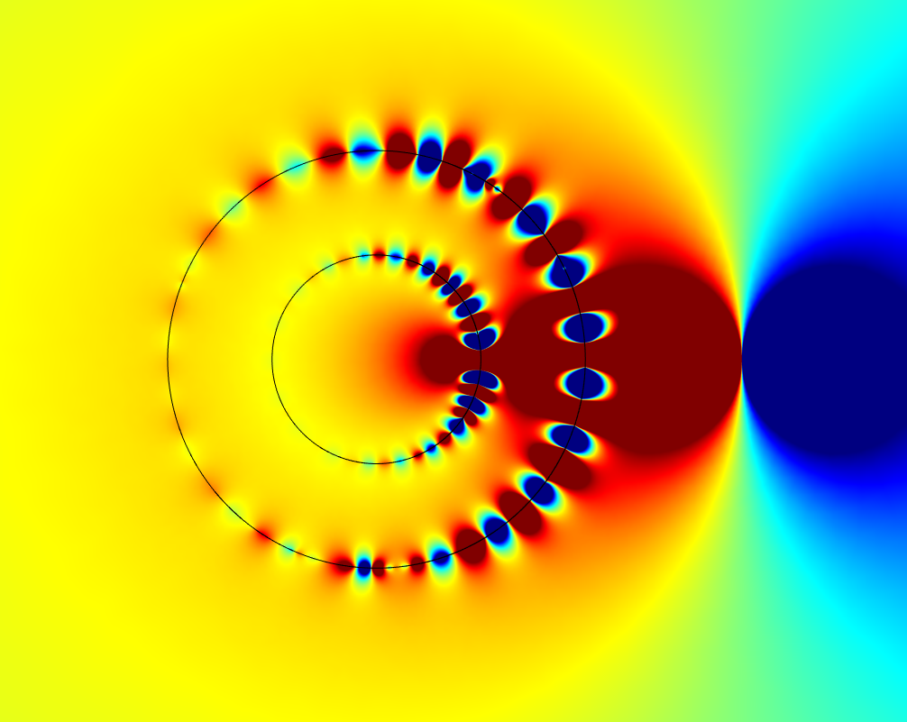
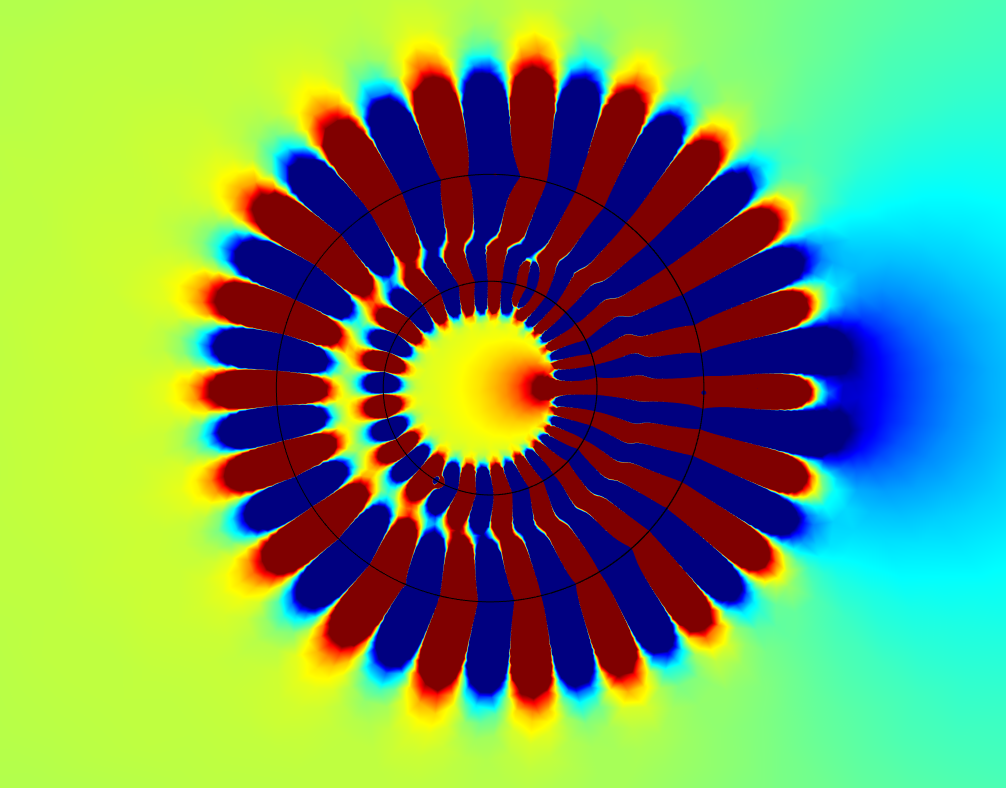
Figure 3: Computational visualization of the occurance of ALR in the electrostatic potential in a quasi-static case that has been observed and analyzed in [22, 23]. The model parameters are $r_{c}=2$, $r_{s}=4$, $\sigma=1\times 10^{-7}$, $\mathbf{p}=\mathbf{u}_{x}p_{x}$. Left panel: $r_{0}=7$, Right panel: $r_{0}=5$.

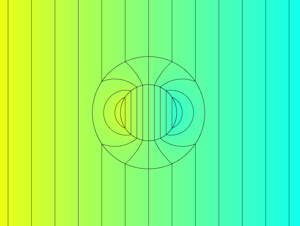
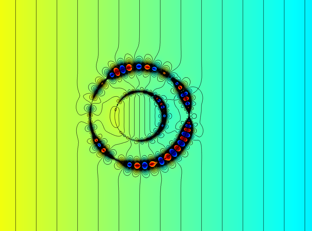
Figure 4: The cloaking based on ALR with quasi-static approximation (for detailed analysis, see [22, 23] and [3]). Potential distribution in the vicinity of a layered cylindrical structure with $r_{c}=1$ and $r_{s}=2$. The permittivity of the annulus $r_{c}<r<r_{s}$ is $\varepsilon_{\text{r}}=-1$. Left: The structure remains invisible in a uniform external field. Right: A small polarized cylinder at $r_{0}=2.5$ excites the ALR in the structure and becomes cloaked.

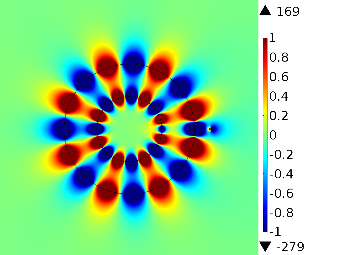
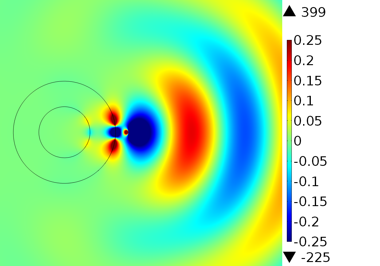
Figure 5: Visualization of the axial magnetic field $H_{z}$ in the electrodynamic case, i.e., without quasi-static approximation. The model parameters are $r_{c}=2$, $r_{s}=4$, $\sigma=1\times 10^{-5}$, $\mathbf{p}=1\mathbf{u}_{y}$ and $r_{0}=5$. Left panel: The frequency is $f=12.5\times 10^{6}$ $(2r_{s}=\lambda/3)$, Right panel: The frequency is $f=37.5\times 10^{6}$ $(2r_{s}=\lambda)$. Note, that our results do not cover the general 2D case i.e. without the quasi-static approximation. This is still an open problem.

Next we consider the electrodynamic case outside the quasistatic regime where the size of the cylindrical structure is no longer significantly small compared with the wavelength. Let us computationally study the geometry setup given in the right panel of Fig. 3 using a radiating line dipole instead of the static one without using the quasi-static approximation. It turns out that for better numerical convergence it is more practical to choose the dipole $\mathbf{u}_{y}$-polarized and increase the material losses to $\sigma=1\times 10^{-5}$. Figure 5 shows the axial magnetic field component $H_{z}$. In the left panel, the frequency ($f=12.5\times 10^{6}$) is chosen such that the outer radius of the cylinder, $2r_{s}$, is one third of the wavelength of the fields radiated by the dipole. A resonance that resembles ALR is still seen occurring in the structure even though its size starts to be comparable with the wavelength. In the right panel ($f=37.5\times 10^{6}$) the radius of the cylinder is exactly one wavelength, $2r_{s}=\lambda$. Here we observe a qualitatively different behavior. Even though a very strong field enhancement is seen on the boundary of the outer annulus in the near vicinity of the dipole, the scattering from the structure is dominant and the localized resonance phenomenon that would cover the the whole structure is absent. Hence, there obviously is an upper limit for the electrical size of the cylindrical structure where the ALR type of resonance is no longer supported. With these particular geometry and material parameters, this happens approximately at $2r_{s}\approx 3\lambda/5.$

Considering an actual realization is this kind of structure, a possible choice for the material of the negative-permittivity annulus could be silver at ultraviolet A range. The permittivity of silver is often described using Drude dispersion model

$$\varepsilon_{\text{Ag}}(\lambda)=\varepsilon_{0}\left(\varepsilon_{\infty}-\frac{(\lambda/\lambda_{p})^{2}}{\bf 1+i\lambda/\lambda_{d}}\right)$$ (5.12)

where $\lambda$ denotes the free-space wavelength. Based on the measured values presented in [16], Ref. [32] applies the model (5.12) with fitted parameters $\varepsilon_{\infty}=5.5$, $\lambda_{p}={\rm 130\,nm}$ and $\lambda_{d}={\rm 30\,nm}$ for wavelength range ${\rm 320\,nm}<\lambda<{\rm 700\,nm}$ (${\rm 430\,THz}\lesssim f\lesssim{\rm 940\,THz}$). At UVA wavelength $\lambda={\rm 331\,nm}$ ($f\approx{\rm 906\,THz}$) this model would give silver the relative permittivity $\varepsilon_{\text{r}}=-1+i0.07.$

Also, it is mentioned in [24] that silicon carbide (SiC) would have a relative permittivity $\varepsilon_{\text{r}}=-1+i0.1$ at much longer infrared wavelength $\lambda={\rm 10.550}\,\mu{\rm m}$ ($f\approx{\rm 28.4\,THz}$).

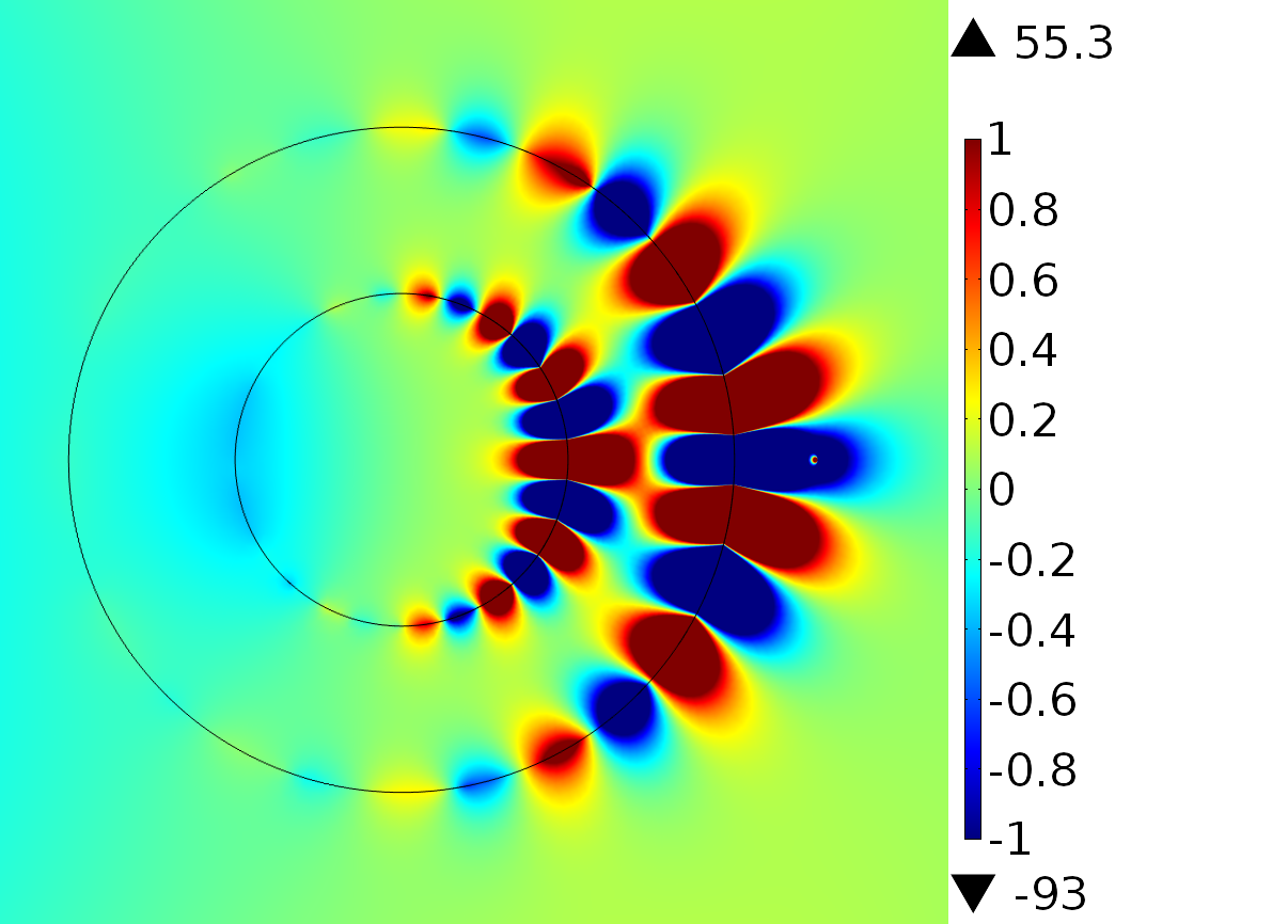
Figure 6: Visualization of the axial magnetic field $H_{z}$ for a double negative 2D layer in the dynamic case. Parameters: $r_{c}=2$, $r_{s}=4$, $r_{0}=5$, $\mathbf{p}=1\mathbf{u}_{y}$ $\varepsilon_{\text{r}}=-1+i1\times 10^{-5}$, $\mu_{r}=-1$, $f=12.5\times 10^{6}$.

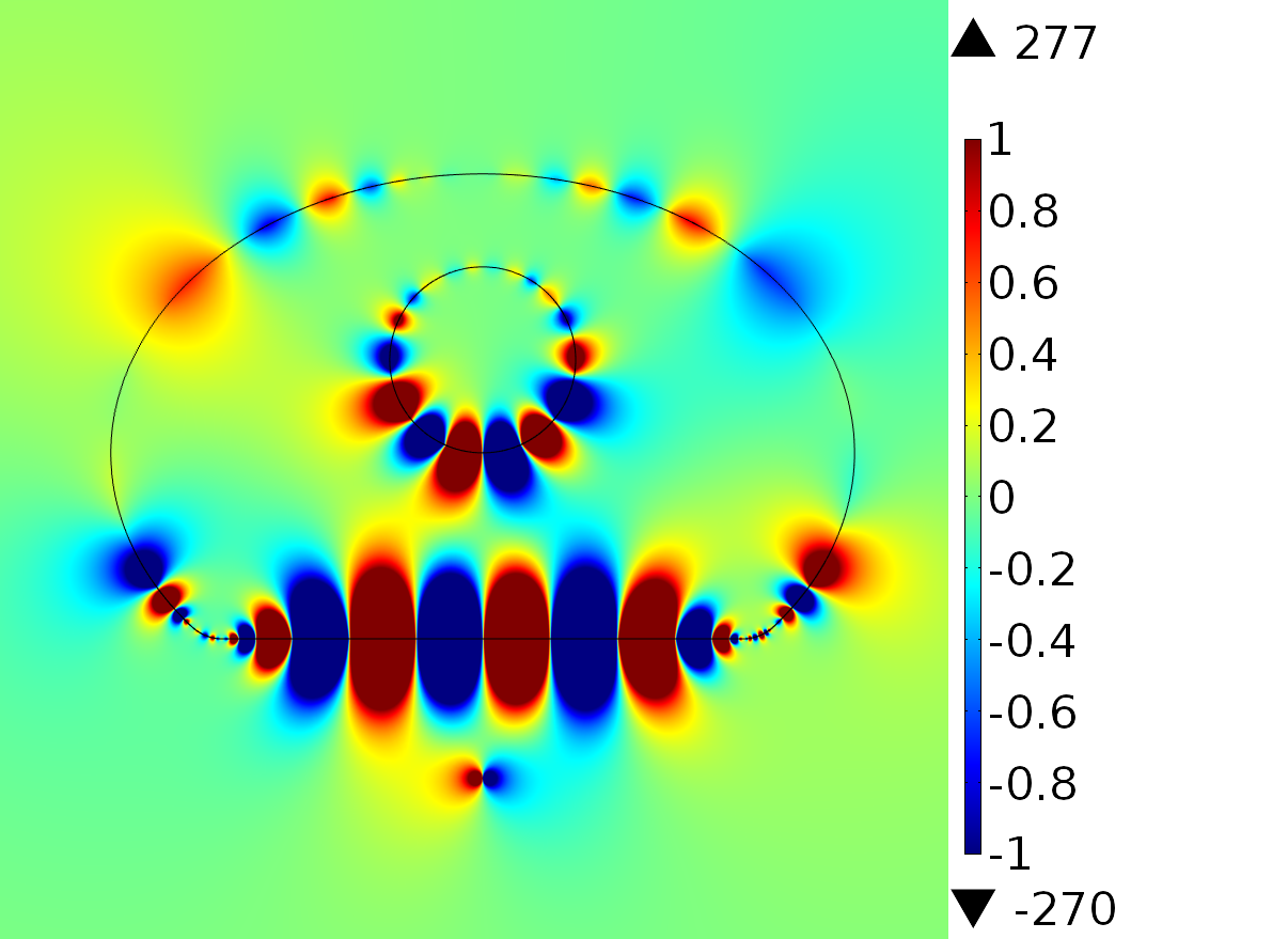
Figure 7: Visualization of the axial magnetic field $H_{z}$ for a 2D double negative domain with a flat part on the boundary. An ellipse semiaxes $a_{s}=4$ and $b_{s}=3$, material parameters $\varepsilon_{\text{r}}=-1+i1\times 10^{-5}$, $\mu=-1$ and a circular hole with radius $r_{c}=1$ is excited by a dipole $\mathbf{p}_{y}=1\mathbf{u}_{y}$ at frequency $f=1.25\times 10^{6}$. The lower part of the ellipse is cut flat, and the resulting corners have been smoothed out. The dipole is located $r_{0}=3.5$ below the center point of the ellipse.

Above it is assumed that only the permittivity of the annulus is negative. In the lossless case with $\varepsilon_{\text{r}}=-1$ and $\mu_{r}=1$, the wave number $k=k_{0}\sqrt{\varepsilon_{\text{r}}}\sqrt{\mu_{r}}$ becomes purely imaginary and no wave propagation inside the annulus is possible. Also, $k^{2}=-k_{0}^{2}$ and the Helmholtz equation (5.10) inside the annulus $r_{s}<r<r_{c}$ reduces to the form

$$(\Delta-k_{0}^{2})H_{z}=0.$$ (5.13)

Instead, if also $\mu_{r}=-1$, the material of the annulus becomes double negative and supports propagating backward waves with negative wave number $k=k_{0}\sqrt{\varepsilon_{\text{r}}}\sqrt{\mu_{r}}=-k_{0}$. The square of $k$ is again positive resulting into the ordinary Helmholtz equation

$$(\Delta+k_{0}^{2})H_{z}=0.$$ (5.14)

Figure 6 visualizes the case for a double negative annulus. The parameters are otherwise the same as in the left panel of Fig. 5, except for $\mu=-1$. We note that in this double negative case, the resonance does not occur symmetrically around the structure, but is more focused in the vicinity of the exciting dipole. Furthermore, the maximum amplitude of the field has decreased. In Fig. 7, the structure is reshaped to resemble the one depicted in Fig. 2. The shape of the outer annulus is elliptic and the center of the inner circular hole is located $0.5$ above the center of the ellipse. Furthermore, the bottom of the ellipse is cut flat, and the resulting corners have been rounded to ensure that the interface remains smooth. The dipole with $\mathbf{p}=1\mathbf{u}_{y}$ is now located $3.5$ below the center of the ellipse. The material parameters and the frequency are the same as in Fig. 6. We note that the strongest resonance is focused on the flat part of the interface.

References

- [1] A. Alù and N. Engheta, Achieving transparency with plasmonic and metamaterial coatings, Phys. Rev. E 72, (2005), 016623.
- [2] H. Ammari, G. Ciraolo, H. Kang, H. Lee, G. W. Milton, Spectral theory of a Neumann–Poincaré -type operator and analysis of cloaking due to anomalous localized resonance. Arch. Ration. Mech. Anal. 208, (2013), 667–692.
- [3] H. Ammari, G. Ciraolo, H. Kang, H. Lee, G. W. Milton, Spectral theory of a Neumann–Poincaré -type operator and analysis of cloaking due to anomalous localized resonance II, Contemporary Mathematics 615, (2014), 1-14.
- [4] H. Ammari, G. Ciraolo, H. Kang, H. Lee, G. W. Milton, Anomalous localized resonance using a folded geometry in three dimensions, Proc. R. Soc. A 469, (2013), 20130048.
- [5] L. Boutet de Monvel, Boundary problems for pseudo-differential operators, Acta Math 126 (1971), 11–51.
- [6] D. Chung, H. Kang, K. Kim, H. Lee, Cloaking due to anomalous localized resonance in plasmonic structures of confocal ellipses, arXiv:1306.6679
- [7] D. L. Colton, R. Kress, Rainer: Integral equation methods in scattering theory. Pure and Applied Mathematics (New York). A Wiley-Interscience Publication. Wiley, New York, 1983.
- [8] M. Costabel, E. Stephan, A direct boundary integral equation method for transmission problems, J. Math. Anal. Appl. 106 (1985), 367–413.
- [9] D. Gilbarg and N. Trudinger, Elliptic partial differential equations of second order. Springer, 2001.
- [10] A. Greenleaf, Y. Kurylev, M. Lassas and G. Uhlmann, Full-wave invisibility of active devices at all frequencies, Comm. Math. Phys. 275 (2007), 749-789.
- [11] A. Greenleaf, Y. Kurylev, M. Lassas and G. Uhlmann, Cloaking devices, electromagnetic wormholes and transformation optics, SIAM Review 51, (2009), 3-33.
- [12] A. Greenleaf, Y. Kurylev, M. Lassas and G. Uhlmann, Invisibility and inverse problems, Bulletin of the American Mathematical Society 46, (2009), 55-97.
- [13] A. Greenleaf, Y. Kurylev, M. Lassas, U. Leonhardt and G. Uhlmann, Cloaked electromagnetic, acoustic, and quantum amplifiers via transformation optics, Proceedings of the National Academy of Sciences (PNAS) 109, (2012), 10169-10174.
- [14] A. Greenleaf, M. Lassas, and G. Uhlmann, Anisotropic conductivities that cannot be detected by EIT, Physiolog. Meas. 24, (special issue on Impedance Tomography), (2003), 413-420.
- [15] A. Greenleaf, M. Lassas and G. Uhlmann, On nonuniqueness for Calderón’s inverse problem, Math. Res. Lett. 10 (2003), 685-693.
- [16] P. B. Johnson and R. W. Christy, Optical constants of the noble metals, Phys. Rev. B 6, (1972), 4370–4379.
- [17] R. E. Kleinman and P. A. Martin, On single integral equations for the transmission problem of acoustics. SIAM J. Appl. Math. 48 (1988), no. 2, 307 325.
- [18] R. V. Kohn, J. Lu, B. Schweizer and M. I. Weinstein, A variational perspective on cloaking by anomalous localized resonance, Comm. Math. Phys. 328 (2014), 1–27.
- [19] R. V. Kohn, D. Onofrei, M. S. Vogelius, M. I. Weinstein, Cloaking via change of variables for the Helmholtz equation, Comm. Pure Appl. Math. 63, (2010), 973–1016.
- [20] R. Kohn, H. Shen, M. Vogelius, and M. Weinstein, Cloaking via change of variables in electrical impedance tomography, Inver. Prob. 24, (2008), 015016.
- [21] W. McLean, Strongly elliptic systems and boundary integral equations, Cambridge University Press, Cambridge, 2000.
- [22] G. W. Milton, N.-A. P. Nicorovici, R. C. McPhedran, and V. A. Podolskiy, A proof of superlensing in the quasistatic regime, and limitations of superlenses in this regime due to anomalous localized resonance, Proc. R. Soc. A 461, (2005), 3999–4034.
- [23] G. W. Milton and N.-A. P. Nicorovici, On the cloaking effects associated with anomalous localized resonance, Proc. R. Soc. A 462, (2006), 3027–3059.
- [24] N. A. Nicorovici, R. C. McPhedran, and G. W. Milton, Optical and dielectric properties of partially resonant composites, Phys. Rev. B 49, (1994), 8479–8482.
- [25] H.-M. Nguyen, A study of negative index materials using transformation optics with applications to super lenses, cloaking, and illusion optics: the scalar case, preprint.
- [26] H.-M. Nguyen and L. H. Nguyen, Localized and complete resonance in plasmonic structures, preprint
- [27] P. Ola, Remarks on a transmission problem. J. Math. Anal. Appl. 196 (1995), 639–658.
- [28] J. B. Pendry, D. Schurig and D.R. Smith, Controlling electromagnetic fields, Science 312, (2006), 1780-1782.
- [29] S. Rempel, B.-W. Schulze, Index theory of elliptic boundary problems, Akademie-Verlag, Berlin, 1982.
- [30] A. Sihvola, Peculiarities in the dielectric response of negative–permittivity scatterers, Progress in Electromagnetic Research, PIERS 66 (2002), 191–198.
- [31] M. E. Taylor, Partial differential equations II. Qualitative studies of linear equations. Second edition. Applied Mathematical Sciences, 116. Springer, New York, 2011.
- [32] H. Wallén, H. Kettunen and A. Sihvola, Composite near-field superlens design using mixing formulas and simulations, Metamaterials 3 (2009), 129–139.
- [33] F. Guevara Vasquez, G. W. Milton, D. Onofrei, Exterior cloaking with active sources in two dimensional acoustics. Wave Motion 48, (2011), 515-524.
- [34] F. Guevara Vasquez, G. W. Milton, D. Onofrei, Mathematical analysis of the two dimensional active exterior cloaking in the quasistatic regime. Anal. Math. Phys. 2 (2012), 231-246.
- [35] G. Uhlmann, Developments in inverse problems since Calderón’s foundational paper, Chapter 19 in Harmonic Analysis and Partial Differential Equations, M. Christ, C. Kenig and C. Sadosky, eds., University of Chicago Press (1999), 295-345. PIE
- [36] G. Uhlmann, Inverse boundary value problems and applications, Astérisque 207(1992), 153–211.