Probabilistic flows of inhabitants in urban areas and self-organization in housing markets

Abstract

We propose a simple probabilistic model to explain the spatial structure of the rent distribution of housing market in city of Sapporo. Here we modify the mathematical model proposed by Gauvin et. al. Nadal . Especially, we consider the competition between two distances, namely, the distance between house and center, and the distance between house and office. Computer simulations are carried out to reveal the self-organized spatial structure appearing in the rent distribution. We also compare the resulting distribution with empirical rent distribution in Sapporo as an example of cities designated by ordinance. We find that the lowest ranking agents (from the viewpoint of the lowest ‘willing to pay’) are swept away from relatively attractive regions and make several their own ‘communities’ at low offering price locations in the city.

1 Introduction

Collective behaviour of interacting animals such as flying birds, moving insects or swimming fishes has attracted a lot of attentions by scientists and engineers due to its highly non-trivial properties. Several remarkable attempts have even done to figure out the mechanism of the collective phenomena by collecting empirical data of flocking of starlings with extensive data analysis Ballerini , by computer simulations of realistic flocking based on a simple algorithm called BOIDS Reynolds ; Makiguchi . Applications of such collective behavior of animals also have been proposed in the context of engineering Olfati .

Apparently, one of the key factors to emerge such non-trivial collective phenomena is ‘local interactions’ between agents. The local interaction in the microscopic level causes non-trivial structures appearing in the macroscopic system. In other words, there is no outstanding leader who designs the whole system, however, the spatio-temporal patterns exhibited by the system are ‘self-organized’ by local decision making of each interacting ingredient in the system.

These sorts of self-organization by means of local interactions between agents might appear not only in natural phenomena but also in some social systems including economics. For instance, decision making of inhabitants in urban areas in order to look for their houses, the resulting organization of residential street (area) and behavior of housing markets are nice examples for such collective behavior and emergent phenomena. People would search suitable location in their city and decide to live a rental (place) if the transaction is approved after negotiation in their own way on the rent with buyers. As the result, the spatio-temporal patterns might be emerged, namely, both expensive and cheap residential areas might be co-existed separately in the city. Namely, local decision makings by ingredients — inhabitants — determine the whole structure of the macroscopic properties of the city, that is to say, the density of residents, the spatial distribution of rent, and behavior of housing markets.

Therefore, it is very important for us definitely to investigate which class of inhabitants chooses which kind of locations, rentals, and what is the main factor for them to decide their housings. The knowledge obtained by answering the above naive questions might be useful when we consider the effective urban planning. Moreover, such a simple but essential question is also important and might be an advanced issue in the context of the so-called spatial economics Fujita .

In fact, constructing new landmarks or shopping districts might encourage inhabitants to move to a new place to live, and at the same time, the resulting distribution of residents induced by the probabilistic flow of inhabitants who are looking for a new place to live might be important information for the administrator to consider future urban planning. Hence, it could be regarded as a typical example of ‘complex systems’ in which macroscopic information (urban planning) and microscopic information (flows of inhabitants to look for a new place to live) are co-evolved in relatively long time scale under weak interactions.

To investigate the macroscopic properties of the system from the microscopic viewpoint, we should investigate the strategy of decision making for individual person. However, it is still extremely difficult for us to tackle the problem by making use of scientifically reliable investigation. This is because there exists quite large person-to-person fluctuation in the observation of individual behaviour. Namely, one cannot overcome the individual variation to find the universal fact in the behaviour even though several attempts based on impression evaluation or questionnaire survey have been done extensively. On the other hand, in our human ‘collective’ behaviour instead of individual, we sometimes observe several universal facts which seem to be suitable materials for computer scientists to figure out the phenomena through sophisticated approaches such as agent-based simulations or multivariate statistics accompanying with machine learning technique.

In a mathematical housing market modeling recently proposed by Gauvin et. al. Nadal , they utilized several assumptions to describe the decision making of each inhabitant in Paris. Namely, they assumed that the intrinsic attractiveness of a city depends on the place and there exists a single peak at the center. They also used the assumption that each inhabitant tends to choose the place where the other inhabitants having the similar or superior income to himself/herself are living. In order to find the best possible place to live, each buyer in the system moves from one place to the other according to the transition (aggregation) probability described by the above two assumption and makes a deal with the seller who presents the best condition for the buyer. They concluded that the resulting self-organized rent distribution is almost consistent with the corresponding empirical evidence in Paris. However, it is hard for us to apply their model directly to the other cities having plural centers (not only a single center as in Paris).

Hence, here we shall modify the Gauvin’s model Nadal to include the much more detail structure of the attractiveness by taking into account the empirical data concerning the housing situation in the city of Sapporo.

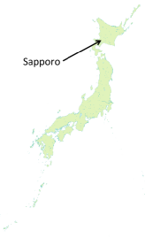
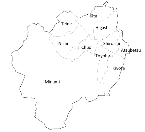
Figure 1: Sapporo is the largest city on the northern Japanese island of Hokkaido. Sapporo is also recognized as one of big cities designated by ordinance and it has ten wards (we call ‘ku’ for ‘ward’ in Japanese), namely, Chuo (Central), Higashi (East), Nishi (West), Minami, Kita (North), Toyohira, Shiraishi, Atsubetsu, Teine and Kiyota.

Sapporo is the fourth-largest city in Japan by population, and the largest city on the northern Japanese island of Hokkaido. Sapporo is also recognized as one of big cities designated by ordinance and it has ten wards (we call ‘ku’ for ‘ward’ in Japanese), namely, Chuo (Central), Higashi (East), Nishi (West), Minami, Kita (North), Toyohira, Shiraishi, Atsubetsu, Teine and Kiyota as shown in Fig. 1.

We also consider the competition between two distances, namely, the distance between house and center, and the distance between house and office. Computer simulations are carried out to reveal the self-organized structure appearing in the rent distribution. Finally, we compare the resulting distribution with empirical rent distribution in Sapporo as an example of cities designated by ordinance. We find that the lowest ranking agents (from the viewpoint of the lowest ‘willing to pay’) are swept away from relatively attractive regions and make several their own ‘communities’ at low offering price locations in the city.

This paper is organized as follows. In the next section 2, we introduce the Gauvin’s model Nadal and attempt to apply it to explain the housing market in city of Sapporo, which is one of typical cites designated by ordinance in Japan. In section 3, we show the empirical distribution of averaged rent in city of Sapporo and compare the distribution with that obtained by computer simulations in the previous section 2. In section 4, we will extend the Gauvin’s model Nadal in which only a single center exists to much more generalized model having multiple centers located on the places of ward offices. In section 5, we definitely find that our generalized model can explain the qualitative behavior of spatial distribution of rent in city of Sapporo. In the same section, we also show several results concerning the office locations of inhabitants and its effect on the decision making of inhabitant moving to a new place. The last section 6 is devoted to summary and discussion.

2 The model system

Here we introduce our model system which was originally proposed by Gauvin et. al. Nadal . We also mention the difficulties we encounter when one applies it to the case of Sapporo city.

2.1 A city — working space —

We define our city as a set of nodes on the $L\times L$ square lattice. The side of each unit of the lattice is $1$ and let us call the set as $\Omega$. From the definition, the number of elements in the set is given by $|\Omega|\equiv L^{2}$. The center of the city is located at $\bm{O}\equiv(L/2,L/2)$. The distance between the center $\bm{O}$ and the arbitrary place in the city, say, $\bm{X}\equiv(x,y)$ is measured by

$$D(\bm{X})=\sqrt{(x-L/2)^{2}+(y-L/2)^{2}}$$ (1)

where we should keep in mind that $D(\bm{X})\leq L/2$ should be satisfied. Therefore, if totally $\mathcal{N}$ rentals are on sale in the city, $N\equiv\mathcal{N}/L^{2}$ houses are put up for sale ‘on average’ at an arbitrary place $\bm{X}$.

Why do we choose city of Sapporo?

As we will see later, our modeling is applicable to any type of city. However, here we choose our home town, city of Sapporo, as a target city to be examined.

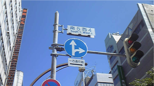
Figure 2: The mark showing where here is in city of Sapporo (urban district). We can easily find it on the top of traffic signal as ‘South 5 West 4’, which means that here is south by 5 blocks, west by 4 blocks from the origin (‘Odori Park’, center).

For the above setting of working space, city of Sapporo is a notable town. This is because the roadways in the urban district are laid to make grid plan road Sapporo . Hence, we can easily specify each location by the two-dimensional vector, say, ‘S5-W4’ which means that south by 5 blocks, west by 4 blocks from the origin (‘Odori Park’, center). Those labels are usually indicated by marks on the top of the traffic signals (see Fig. 2). These kinds of properties might help us to collect the empirical data sets and compare them with the outputs from our probabilistic model.

2.2 Agents

We suppose that there co-exist three distinct agents, namely, ‘buyers’, ‘sellers’ and ‘housed’. The total number of these agents is not constant but changing in time. For instance, in each (unit) time step $t=1$, $\Gamma\,\,(\geq 1)$ agents visit to the city as ‘new buyers’, whereas $\alpha$ percentage of the total housed persons let the house go for some amount of money and they become ‘new sellers’. When the ‘new sellers’ succeeded in selling their houses, they leave the city to move to the other cities. The situation is illustrated by a cartoon in Fig. 3.

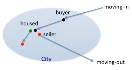
Figure 3: Three kinds of agents in our model system and those typical behaviors. A newcomer as a ‘buyer’ looks for the housing in the city (say, Sapporo). The ‘housed’ who is living his/her own house becomes a ‘seller’ when he/she would move to the other city (e.g., Tokyo or Osaka). Each seller presents the possible rent to the buyers. Once the seller accepts the offer price and makes a contract with the buyer, the buyer becomes a ‘housed’ at the place and the seller immediately leaves from the city (Sapporo).

Ranking of agents

Each of agent is categorized (ranked) according to their degree of ‘willing to pay’ for the housing. Let us define the total number of categories by $K$. Then, the agent belonging to the category $k\in\{0,\cdots,K-1\}$ can pay $P_{k}$ (measured by a currency unit, for instance Japanese yen) for the housing. Hence, we can give the explicit ranking to all agents when we put the price $P_{k}$ in the following order

$$P_{0}<P_{1}<\cdots<P_{K-1}.$$ (2)

In this paper, the price $P_{k}$ of ‘willing to pay’ is given by

$$P_{k}=P_{0}+k\,\frac{\Delta}{K-1},\,\,\,k=0,\cdots,K-1,$$ (3)

namely, as the difference between the highest rent $P_{0}$ and the lowest $P_{K-1}$ leads to a gap $\Delta$, each category (person) is put into one of the $\Delta/K$ intervals. In our computer simulations which would be given later on, the ranking of each agent is allocated randomly from $\{0,\cdots,K-1\}$.

2.3 Attractiveness of locations

A lot of persons are attracted by specific areas close to the railway (subway) stations or big shopping districts for housing. As well-known, especially in city of Sapporo, Maruyama-area which is located in the west side of the Sapporo railway station has been appealed to, in particular, high-ranked persons as an exclusive residential district. Therefore, one can naturally assume that each area in the city possesses its own attractiveness and we might regard the attractiveness as time-independent quantity.

However, the attractiveness might be also dependent on the categories (ranking) of agents in some sense. For instance, the exclusive residential district is not attractive for some persons who have relatively lower income and cannot afford the house. On the other hand, some persons who have relatively higher income do not want to live the area where is close to the busy street or the slum areas.

Taking into account these two distinct facts, the resulting attractiveness for the area $\bm{X}$ should consists of the part of the intrinsic attractiveness $A^{0}(\bm{X})$ which is independent of the categories $k=0,\cdots,K-1$ and the another part of the attractiveness which depends on the categories. Hence, we assume that attractiveness at time $t$ for the person who belongs to the category $k$ at the area $\bm{X}$, that is, $A_{k}(\bm{X},t)$ is updated by the following spatio-temporal recursion relation:

$$A_{k}(\bm{X},t+1)=A_{k}(\bm{X},t)+\omega(A^{0}(\bm{X})-A_{k}(\bm{X},t))+\Phi_{k}(\bm{X},t)$$ (4)

where $A^{0}(\bm{X})$ stands for the time-independent intrinsic attractiveness for which any person belonging to any category feels the same amount of charm.

For example, if the center of the city $\bm{O}=(L/2,L/2)$ possesses the highest intrinsic attractiveness $A^{0}_{\rm max}$ as in Paris Nadal , we might choose the attractiveness $A^{0}(\bm{X})$ as a two-dimensional Gaussian distribution with mean $\bm{O}=(L/2,L/2)$ and the variance $R^{2}$ as

$$A^{0}(\bm{X})=\frac{A^{0}_{\rm max}}{\sqrt{2\pi R^{2}}}\,{\exp}\left[-\frac{\{(x-L/2)^{2}+(y-L/2)^{2}\}}{2R^{2}}\right]$$ (5)

where the variance $R^{2}$ denotes a parameter which controls the range of influence from the center. We should notice that the equation (4) has a unique solution $A^{0}(\bm{X})$ as a steady state when we set $\Phi_{k}(\bm{X},t)=0$.

Incidentally, it is very hard for us to imagine that there exist direct interactions (that is, ‘communications’) between agents who are looking for their own houses. However, nobody doubts that children’s education (schools) or public peace should be an important issue for persons (parents) to look for their housing. In fact, some persons think that their children should be brought up in a favorable environment with their son’s/daughter’s friends of the same living standard as themselves. On the other hand, it might be rare for persons to move to the area where a lot of people who are lower living standard than themselves. Namely, it is naturally assumed that people seek for the area as their housing place where the other people who are higher living standard than themselves are living, and if possible, they would like to move such area.

Hence, here we introduce such ‘collective effects’ into the model system by choosing the term $\Phi_{k}(\bm{X},t)$ as

$$\Phi_{k}(\bm{X},t)=\epsilon\sum_{k^{{}^{\prime}}\geq k}v_{k^{{}^{\prime}}}(\bm{X},t)$$ (6)

where $v_{k}(\bm{X},t)$ stands for the density of housed persons who are in the category $k$ at the area $\bm{X}$ at time $t$. Namely, from equations (4) and (6), the attractiveness of the area $\bm{X}$ for the people of ranking $k$, that is, $A_{k}(\bm{X},t)$ increases at the next time step $t+1$ when persons who are in the same as or higher ranking than $k$ start to live at $\bm{X}$. It should bear in mind that the intrinsic part of attractiveness $A^{0}(\bm{X})$ is time-independent, whereas $\Phi_{k}(\bm{X},t)$ is time-dependent through the flows of inhabitants in the city. Thus, the $A_{k}(\bm{X},t)$ could have a different shape from the intrinsic part $A^{0}(\bm{X})$ due to the effect of the collective behavior of inhabitants $\Phi_{k}(\bm{X},t)$.

2.4 Probabilistic search of locations by buyers

The buyers who have not yet determined their own house should look for the location. Here we assume that they move to an arbitrary area ‘stochastically’ according to the following probability:

$$\pi_{k}(\bm{X},t)=\frac{1-{\exp}(-\lambda A_{k}(\bm{X},t))}{\sum_{\bm{X}^{{}^{\prime}}\in\Omega}\{1-{\exp}(-\lambda A_{k}(\bm{X}^{{}^{\prime}},t))\}}$$ (7)

Namely, the buyers move to the location $\bm{X}$ to look for their housing according to the above probability. The situation is shown as a cartoon in Fig. 4.

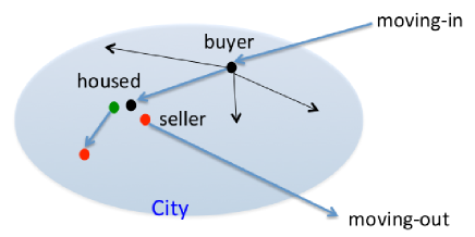
Figure 4: In each time step, a buyer visits a place $\bm{X}$ with a probability (7). By repeating the transition processes, a buyer explores the suitable and desirable location in the city from place to place.

We easily find from equation (7) that for arbitrary $\lambda$, the area which exhibits relatively high attractiveness is more likely to be selected as a candidate to visit at the next round. Especially, in the limit of $\lambda\to\infty$, the buyers who are looking for the locations visit only the highest attractiveness location

$$\bm{X}_{k}={\rm argmax}_{\bm{X}}A_{k}(\bm{X},t).$$ (8)

On the other hand, for $\lambda\ll 1$, equation (7) leads to

$$\pi_{k}(\bm{X},t)=\frac{A_{k}(\bm{X},t)}{\sum_{\bm{X}^{{}^{\prime}}\in\Omega}A_{k}(\bm{X}^{{}^{\prime}},t)},$$ (9)

and the probability for buyers to visit the place $\bm{X}$ at time $t$ is proportional to the attractiveness corresponding to the same area $A_{k}(\bm{X},t)$.

Here we should mention that when we regard the ‘location’ as ‘company’, the present model system is described by similar aggregation probability to the probabilistic labor market proposed by Chen et. al. Chen where the parameter $\gamma$ corresponds to the $\lambda$ in the Gauvin’s model Nadal .

2.5 Offering prices by sellers

It is not always possible for buyers to live at the location $\bm{X}$ where they have selected to visit according to the probability $\pi_{k}(\bm{X},t)$ because it is not clear whether they can accept the price offered by the sellers at $\bm{X}$ or not. Obviously, the offering price itself depends on the ranking $k$ of the sellers. Hence, here we assume that the sellers of ranking $k$ at the location $\bm{X}$ offer the buyers the price:

$$P_{k}^{o}(\bm{X})=P^{0}+[1-{\exp}(-\xi\overline{A}(\bm{X},t))]P_{k}$$ (10)

for the rental housing, where $\overline{A}(\bm{X},t)$ means the average of the attractiveness $A_{k}(\bm{X},t)$ over the all categories $k=0,\cdots,K-1$, that is to say,

$$\overline{A}(\bm{X},t)\equiv\frac{1}{K}\sum_{k=0}^{K-1}A_{k}(\bm{X},t),$$ (11)

and $\xi$ is a control parameter. In the limit of $\xi\to\infty$, the offering price by a seller of ranking $k$ is given by the sum of the basic rent $P^{0}$ and the price of ‘willing to pay’ for the sellers of ranking $k$, namely, $P_{k}$ as $P_{k}^{o}=P^{0}+P_{k}$.

For the location $\bm{X}$ in which any transaction has not yet been approved, the offering price is given as

$$P_{k}^{o}(\bm{X})=P^{0}+[1-{\exp}(-\xi\overline{A}(\bm{X},t))]P^{1}$$ (12)

because the ranking of the sellers is ambiguous for such location $\bm{X}$.

2.6 The condition on which the transaction is approved

It is needed for buyers to accept the price offered by sellers in order to approve the transaction. However, if the offering price is higher than the price of ‘willing to pay’ for the buyer, the buyer cannot accept the offer. Taking into account this limitation, we assume that the following condition between the buyer of the ranking $k$ and the seller of the ranking $k^{{}^{\prime}}$ at the location $\bm{X}$ should be satisfied to approve the transaction.

$$P_{k}>P_{k^{{}^{\prime}}}^{o}(\bm{X})$$ (13)

Thus, if and only if the above condition (13) is satisfied, the buyer can own the housing (the seller can sell the housing).

We should keep in mind that there is a possibility for the lowest ranking people to fail to own any housing in the city even if they negotiate with the person who also belongs to the lowest ranking. To consider the case more carefully, let us set $k=k^{{}^{\prime}}=0$ in the condition (13), and then we have $P_{0}>{P^{0}}/{{\exp}[-\xi\overline{A}(\bm{X},t)]}$. Hence, for the price of ‘willing to pay’ $P_{0}$ of the lowest ranking people, we should determine the lowest rent $P^{0}$ so as to satisfy $P^{0}<{\exp}[-\xi\overline{A}(\tilde{\bm{X}},t)]P_{0}$. Then, the lowest ranking people never fail to live in the city.

We next define the actual transaction price as interior division point between $P_{k}$ and $P_{k^{{}^{\prime}}}^{o}(\bm{X})$ by using a single parameter $\beta$ as

$$P_{\rm tr}=(1-\beta)P_{k^{{}^{\prime}}}(\bm{X})+\beta P_{k}.$$ (14)

By repeating these three steps, namely, probabilistic searching of the location by buyers, offering the rent by sellers, transaction between buyers and sellers for enough times, we evaluate the average rent at each location $\bm{X}$ and draw the density of inhabitants, the spatial distribution of the average rent in two-dimension. In following, we show our preliminary results.

2.7 Computer simulations: A preliminary

In Fig. 5, we show the spatial density distribution $\rho(r)$ of inhabitants by the Gauvin’s model Nadal having a single center in the city. The horizontal axis $r$ of these panels stands for the distance between the center $\bm{O}$ and the location $\bm{X}$, namely, $r=D(\bm{X})$. We set the parameters appearing in the model as $L=100,\alpha=0.1,K=10,P_{0}=15,000,\Delta+P_{0}=120,000\,(\Delta=105,000),\omega=1/15,R=10,\epsilon=0.0022,\lambda=0.01,\zeta=0.1,P^{0}=9,000,P^{1}=200,000,\beta=0.1,\Gamma=L^{2}/K,\\ T=100\,(\equiv\mbox{Total number of updates (\ref{eq:update})})$. It should be noted that the definition of density is given by

$$\rho(r)\equiv\frac{\mbox{($\#$ of inhabitants of ranking $k$ at the location $r$)}}{\mbox{(Total $\#$ of inhabitants at the location $r$)}}.$$ (15)

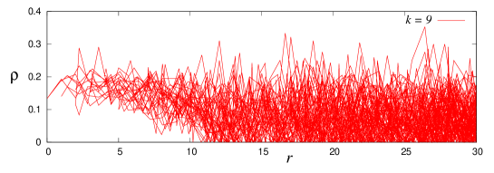
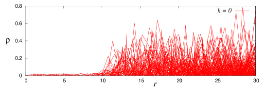
Figure 5: The spatial density $\rho(r)$ of inhabitants obtained by the Gauvin’s model Nadal having a single center in the city. The horizontal axis $r$ stands for the distance between the center $\bm{O}=(L/2,L/2)$ and the location $\bm{X}=(x,y)$, namely, $r=D(\bm{X})$. The upper panel is the result for the highest raining people ($k=K-1$), whereas the lower panel shows the result for the lowest ranking inhabitants ($k=0$). We easily recognize that the persons who are belonging to the lowest ranking cannot live the area close to the center.

From the lower panel, we easily recognize that the persons who are belonging to the lowest ranking cannot live the area close to the center in the city. Thus, we find that there exists a clear division of inhabitants of different rankings.

Intuitively, these phenomena might be understood as follows. The persons of the highest ranking ($k=K-1$) can afford to accept any offering price at any location. At the same time, the effect of aggregation induced by $\Phi_{K-1}(\bm{X},t)$ in the searching probability $\pi_{K-1}(\bm{X},t)$ and the update rule of $A_{K-1}(\bm{X},t)$ in (4) is the weakest among the $K$ categories. As the result, the steady state of the update rule (4) is not so deviated from the intrinsic attractiveness, namely, $A_{K-1}(\mbox{\boldmath$X$},t)\simeq A^{0}(\bm{X})$. Hence, people of the highest ranking are more likely to visit the locations where are close to the center $\bm{X}=\bm{O}$ and they live there. Of course, the density of the highest ranking persons decreases as $r$ increases.

On the other hand, people of the lowest ranking ($k=0$) frequently visit the locations where various ranking people are living due to the aggregation effect of the term $\Phi_{0}(\bm{X},t)$ to look for their housing. However, it is strongly dependent on the offering price at the location whether the persons can live there or not. Namely, the successful rate of transaction depends on which ranking buyer offers the price at the place $\bm{X}$. For the case in which the ‘housed’ people changed to sellers at the location where is close to the center, the seller is more likely to be the highest ranking person because he/she was originally an inhabitant owing the house near the center. As the result, the price offered by them might be too high for the people of the lowest ranking to pay for approving the transaction. Therefore, the lowest raining people might be driven away to the location where is far from the center.

3 Empirical data in city of Sapporo

Apparently, the above simple modeling with a single center of city is limited to the specific class of city like Paris. Turning now to the situation in Japan, there are several major cites designated by ordinance, and city of Sapporo is one of such ‘mega cities’. In Table 1, we show several statistics in Sapporo in 2010. From this table, we recognize that in each year, 63,021 persons are moving into and 57,587 persons are moving out from Sapporo. Hence, the population in Sapporo is still increasing by approximately six thousand in each year.

Wards	$\#$ of moving-in	$\#$ of moving-out	lowest (yen)	highest (yen)
Chuo (Central)	12,132	10,336	19,000	120,000
Kita (North)	8,290	7,970	15,000	73,000
Higashi (East)	7,768	7,218	20,000	78,500
Shiraishi	6,857	6,239	25,000	67,000
Atsubetsu	4,003	3,736	33,000	57,000
Toyohira	7,854	7,037	20,000	69,000
Kiyota	2,560	2,398	30,000	55,000
Minami (South)	3,824	3,794	23,000	58,000
Nishi	6,315	5,788	20,000	80,000
Teine	3,418	3,071	20,000	68,000
Total	63,021	57,587	—	—

Table 1: Statistics in city of Sapporo for the number of persons who were moving-into and -out, the lowest and highest rents (the unit is Japanese yen) of 2DK-type flats in city of Sapporo.

As we already mentioned, Sapporo is the fourth-largest city in Japan by population, and the largest city on the northern Japanese island of Hokkaido. Sapporo is recognized as one of big cities designated by ordinance and it has ten wards (what we call ‘ku’ in Japanese), namely, Chuo, Higashi, Nishi, Minami, Kita, Toyohira, Shiraishi, Atsubetsu, Teine and Kiyota as shown in Table 1 (for details, see Sapporo for example). Hokkaido prefectural office is located in Chuo-ku and the other important landmarks concentrate in the wards. Moreover, as it is shown in Table 1, the highest and the lowest rents for the 2DK-type (namely, a two-room apartment with a kitchen/dining area) flats in Chuo-ku are both the highest among ten wards. In this sense, Chuo-ku could be regarded as a ‘center’ of Sapporo. However, the geographical structure of rent distribution in city of Sapporo is far from the symmetric one as given by the intrinsic attractiveness $A^{0}(\bm{X})$ having a single center (see equation (5)). In fact, we show the rough distribution of average rents in city of Sapporo in Fig.6 by making use of the empirical data collected from Souba . From this figure, we clearly confirm that the spatial structure of rents in city of Sapporo is not symmetric but apparently asymmetric.

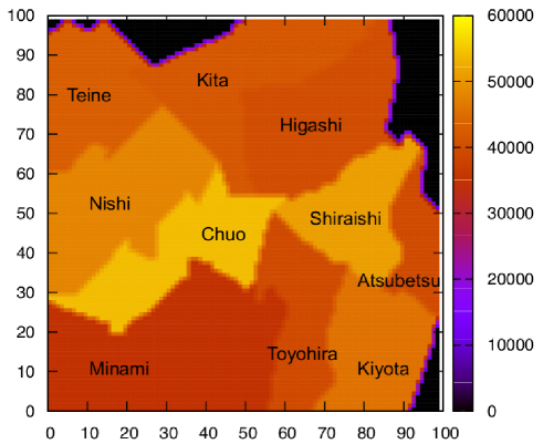
Figure 6: The spatial distribution of the averaged rent in city of Sapporo by using the empirical housing data collected from Souba . In Sapporo, ten wards Chuo (Central), Higashi (East), Nishi (West), Minami (South), Kita, Toyohira, Shiraishi, Atsubetsu, Teine and Kiyota exist. (COLOR ONLINE)

From this distribution, we also find that the average rent is dependent on wards, and actually it is very hard to simulate the similar spatial distribution by using the Gauvin’s model Nadal in which there exists only a single center in the city. This is because in a city designated by ordinance like Sapporo, each ward formulates its own community, and in this sense, each ward should be regarded as a ‘small city’ having a single (or multiple) center(s). It might be one of the essential differences between Paris and Sapporo.

4 An extension to a city having multiple centers

In the previous section 3, we found that the Gauvin’s model Nadal having only a single center is not suitable to explain the empirical evidence for a city designated by ordinance such as Sapporo where multiple centers as wards co-exist.

Therefore, in this section, we modify the intrinsic attractiveness $A^{0}(\bm{X})$ to explain the empirical evidence in city of Sapporo. For this purpose, we use the label $l=1,\cdots,10$ to distinguish ten words in Sapporo, namely, Chuo (Central), Higashi (East), Nishi (West), Minami (South), Kita (North), Toyohira, Shiraishi, Atsubetsu, Teine and Kiyota in this order, and define $\bm{B}_{l}=(x_{B_{l}},y_{B_{l}}),l=1,\cdots,10$ for each location where each ward office is located. Then, we shall modify the intrinsic attractiveness in terms of the $\bm{B}_{l}$ as follows.

$$A^{0}(\bm{X})=\sum_{l=1}^{10}\frac{\delta_{l}}{\sqrt{2\pi}R_{l}}{\exp}\left[-\frac{\{(x-x_{B_{l}})^{2}+(y-y_{B_{l}})^{2}\}}{2R_{l}^{2}}\right]$$ (16)

where

$$\delta_{1}+\cdots+\delta_{10}=1$$ (17)

should be satisfied. Namely, we would represent the intrinsic attractiveness $A^{0}(\bm{X})$ in city of Sapporo by means of a two-dimensional mixture of Gaussians in which each mean corresponds to the location of the ward office. $R_{l}\,(l=1,\cdots,10)$ denotes a set of parameters which control the spread of the center. In our computer simulations, we set $R_{l}=5$ for all $l=1,\cdots,10$ in our intrinsic attractiveness (16).

Here we encounter a problem, namely, we should choose each weight $\delta_{l},\,l=1,\cdots,10$. For this purpose, we see the number of estates (flats) in each wards. From a real-estate agents in Sapporo Homes , we have the statistics as Chuo (Central) ($9,598$), Higashi (East) ($6,433$), Nishi (West) ($5,830$), Minami (South) ($1,634$), Kita (North) ($4,671$), Toyohira ($4,893$), Shiraishi ($5,335$), Atsubetsu ($1,104$), Teine ($2,094$), Kiyota ($962$). Hence, by dividing each number by the maximum $9,598$ for Chuo-ku, the weights $\delta_{l},\,l=1,\cdots,10$ are chosen as Chuo (Central) ($\delta_{1}\propto 1.0$), Higashi (East) ($\delta_{2}\propto 0.67$), Nishi (West) ($\delta_{3}\propto 0.61$), Minami (South) ($\delta_{4}\propto 0.17$), Kita (North) ($\delta_{5}\propto 0.49$), Toyohira ($\delta_{6}\propto 0.51$), Shiraishi ($\delta_{7}\propto 0.56$), Atsubetsu ($\delta_{8}\propto 0.12$), Teine ($\delta_{9}\propto 0.22$), Kiyota ($\delta_{10}\propto 0.1$). Of course, we normalize these parameters so as to satisfy the condition (17).

5 Computer simulations

In this section, we show the results of computer simulations.

5.1 Spatial structure in the distribution of visiting times

In Fig. 7 (left), we show the distributions of the number of persons who checked the information about the flat located at $\bm{X}$ and the number of persons who visited the place $\bm{X}$ according to the transition probability (7) in the right panel. From this figure, we find that the locations (flats) $\bm{X}$ where people checked on the web site Homes most frequently concentrate around each ward office. From this fact, our modeling in which we choose the locations of multiple centers as the places of wards might be approved. Actually, from the right panel of this figure, we are confirmed that the structure of spatial distribution is qualitatively very similar to the counter-empirical distribution (right panel).

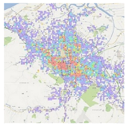
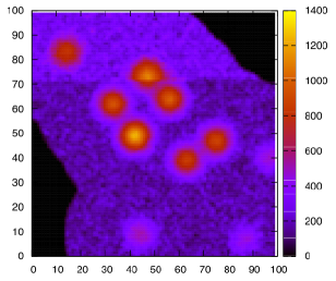
Figure 7: The distributions of the number of persons who checked the information about the flat located at $\bm{X}$ on the web site (left, from Homes ) and the number of persons who visited the place $\bm{X}$ according to the transition probability (7) (right) in our artificial society. (COLOR ONLINE)

In order to investigate the explicit ranking dependence of the housing-search behavior of agents, in Fig. 8 (the upper panels), we plot the spatial distribution of the number of visits for the lowest ranking $k=0$ (left) and the highest ranking $k=9$ (right) agents. We also plot the corresponding spatial distributions of the number of the transaction approvals in the lower two panels. From this figure, we confirm that the lowest ranking agents visit almost whole area of the city, whereas the highest ranking agents narrow down their visiting place for housing search. This result is naturally understood as follows. Although the lowest ranking agents visit some suitable places to live, they cannot afford to accept the offer price given by the sellers who are selling the flats at the place. As the result, such lowest ranking agents should wander from place to place to look for the place where the offer price is low enough for them to accept. That is a reason why the spatial distribution of visit for the lowest ranking agents distributes widely in the city. On the other hand, the highest ranking agents posses enough ‘willing to pay’ $P_{9}$ and they could live any place they want. Therefore, their transactions are easily approved even at the centers of wards with relatively high intrinsic attractiveness $A^{0}(\bm{X})$.

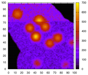
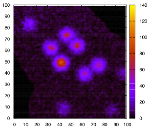
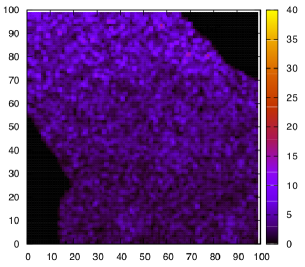
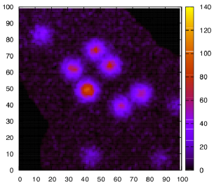
Figure 8: The upper two panels show the spatial distribution of the number of visits consisting of the lowest ranking $k=0$ (left) and the highest ranking $k=9$ (right) agents. The corresponding spatial distributions of the number of the transaction approvals are shown in the lower panels. (COLOR ONLINE)

As a non-trivial finding, it should be noticed from Fig. 8 that in the northern part of the city (a part of Kita and Higashi-ku), several small communities consisting of the lowest ranking persons having their ‘willing to pay’ $P_{0}$ emerge. In our modeling, we do not use any ‘built-in’ factor to generate this sort of non-trivial structure. This result might imply that communities of poor persons could be emerged in any city in any country even like Japan.

Let us summarize our findings from simulation concerning ranking dependence of search-approvals by agents below.

• The lowest ranking agents ($k=0$) visit almost all of regions in city even though such places are highly ‘attractive places’.

• The highest ranking agents ($k=9$) visit relatively high attractive places. The highest ranking agents are rich enough to afford to accept any offering price, namely, $\#$ of contracts $\simeq$ $\#$ of visits.

• The lowest ranking agents are swept away from relatively attractive regions and make several their own ‘communities’ at low offering price locations in the city (the north-east area in Sapporo).

5.2 The rent distribution

In Fig. 9 (left), we plot the resulting spatial distribution of rent in city of Sapporo. From this figure we confirm that the spatial distribution is quantitatively similar to the empirical evidence. We also find that a complicated structure — a sort of spatial anisotropy — emerges and it is completely different from the result by the Gauvin’s model Nadal . In particular, we should notice that relatively high rent regions around Chuo-ku appear. These regions are located near Kita, Higashi, Nishi and Shiraishi.

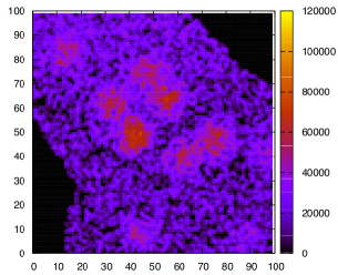
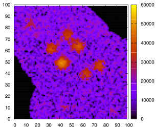
Figure 9: The resulting spatial distributions of rent in city of Sapporo. In the left panel, we do not consider the effect of office locations on buyer’s decision, whereas in the right panel, the effect is taken into account. (COLOR ONLINE)

To see the gap between our result and empirical evidence quantitatively, we show the simulated average rent and the counter-empirical evidence in Table 2. From this table, we find that the order of the top two wards simulated by our model, namely, Chuo and Shiraishi coincides with the empirical evidence, and moreover, the simulated rent itself is very close to the market price. However, concerning the order of the other wards, it is very hard for us to conclude that the model simulates the empirical data. Of course, the market price differences in those wards are very small and it is very difficult to simulate the correct ranking at present. Thus, the modification of our model to generate the correct ranking and to obtain the simulated rents which are much closer to the market prices should be addressed our future study.

ranking	market price (yen)
Chuo (Central)	54,200
Shiraishi	51,100
Nishi (West)	48,200
Kiyota	45,800
Teine	42,900
Kita (North)	41,700
Higashi (East)	40,100
Atsubetsu	39,700
Toyohira	39,600
Minami (South)	34,400

ranking	simulated average rent (yen)
Chuo (Central)	50,823
Shiraishi	43,550
Higashi (East)	44,530
Kita (North)	43,516
Nishi (West)	43,093
Toyohira	42,834
Minami (South)	39,909
Teine	39,775
Kiyota	37,041
Atsubetsu	36,711

Table 2: The left list shows the ranking (order) and the market prices. The simulated average rent for each ward and the ranking are shown in the right list. The unit of price is Japanese yen Homes .

5.3 On the locations of offices

In the previous sections, we modified the intrinsic attractiveness so as to possess the multiple peaks at the corresponding locations of the ward offices by (16). However, inhabitants must go to their office every weekday, and the location of office might give some impact on the decision making of each buyer in the city. For a lot of inhabitants in Sapporo city, their offices are located within the city, however, the locations are distributed. Hence, here we specify the ward in which his/her office is located by the label $m=1,\cdots,10$ and rewrite the intrinsic attractiveness (16) as

$$A_{m}^{0}(\bm{X}) = \sum_{l\neq m}^{10}\frac{\delta_{l}}{\sqrt{2\pi}R_{l}}{\exp}\left[-\frac{\{(x-x_{B_{l}})^{2}+(y-y_{B_{l}})^{2}\}}{2R_{l}^{2}}\right]$$

$$+ \frac{(\delta_{m}+\eta)}{\sqrt{2\pi}R_{m}}{\exp}\left[-\frac{\{(x-x_{B_{m}})^{2}+(y-y_{B_{m}})^{2}\}}{2R_{m}^{2}}\right].$$

Namely, for the buyer who has his/her office within the ward $m$, the ward $m$ might be a ‘special region’ for him/her and the local peak appearing in the intrinsic attractiveness is corrected by $\eta$. If he/she seeks for the housing close to his/her house (because the commuting cost is high if the office is far from his/her house), the correction $\eta$ takes a positive value. On the other hand, if the buyer wants to live the place located far from the office for some reasons (for instance, some people want to vary the pace of their life), the correction $\eta$ should be negative. To take into account these naive assumptions, we might choose $\eta$ as a snapshot from a Gaussian with mean zero and the variance $\sigma^{2}(<\delta_{m})$. From this type of corrections, the buyer, in particular, the buyer of the highest ranking ($k=K-1$) might feel some ‘frustration’ to make their decision, which is better location for them between Chuo-ku as the most attractive ward and the ward $m$ where his/her office is located under the condition $\delta_{1}\simeq\delta_{m}+\eta$. For the set of weights $\delta_{m},\,m=1,\cdots,10$, we take into account the number of offices in each ward, that is, Chuo (23,506), Kita (8,384), Higashi (8,396), Shiraishi (7,444), Toyohira (6.652), Minami (3,418), Nishi (6,599), Atsubetsu (2,633), Teine (3,259), Kiyota (2,546). Then, we choose each $\delta_{m}$ by dividing each number by the maximum of Chuo-ku as Chuo ($\delta_{1}\propto 1.00$), Higashi ($\delta_{2}\propto 0.36$), Nishi ($\delta_{3}\propto 0.28$), Minami ($\delta_{4}\propto 0.15$), Kita ($\delta_{5}\propto 0.36$), Toyohira ($\delta_{6}\propto 0.28$), Shiraishi ($\delta_{7}\propto 0.32$), Atsubetsu ($\delta_{8}\propto 0.11$), Teine ($\delta_{9}\propto 0.14$), Kiyota ($\delta_{10}\propto 0.11$). For the bias parameter $\eta$, we pick up the value randomly from the range:

$$|\eta|<\delta_{m},$$ (18)

instead of the Gaussian.

The resulting spatial distribution is shown in the right panel of Fig. 9. From this panel, we are clearly confirmed that the spatial structure of rents distributes more widely in whole city than that without taking into account the office location (see the left panel in Fig. 9 for comparison). We should notice that the range of simulated rent in the city is remarkably reduced from $[0,120,000]$ to $[0,60,000]$ due to the diversification of values to consider the location of their housing.

5.4 On the effective time-scale of update rule

Until now, we did not make a mention of time scale in the spatio-temporal update rule (4) in the attractiveness $A_{k}(\bm{X},t)$. However, it might be important to for us consider how long the time in our model system (artificial society) goes on for the minimum time step $t\to t+1$, especially when we evaluate the necessary period of time to complete the accumulation of community after new-landmarks or shopping mall come out. To decide the effective time-scale for $t\to t+1$, we use the information about the number of persons moving-into city of Sapporo through the year. Let us define the number from the empirical data by $C$. Then, we should remember that in our simulation, we assumed that in each time step ($t\to t+1$), $\Gamma$ newcomers visit the city. Hence, the actual time $\tau$ for the minimum time step $t\to t+1$ in our artificial society is effectively given by

$$\tau=365\times\frac{\Gamma}{C}\,\,[\mbox{days}].$$ (19)

Therefore, by using our original set-up $\Gamma\equiv L^{2}/K=(100\times 100)/10=1000$ and by making use of the data listed in Table 1, we obtain $C=63021$, and substituting the value into (19), we finally have $\tau=(1000\times 365)/63021=5.79$ [days] for $t\to t+1$. This means that approximately 579 days have passed when we repeat the spatio-temporal update rule (4) by $T=100$ times. This information might be essential when we predict the future housing market, let us say, after constructing the Hokkaido Shinkansen (a rapid express in Japan) railway station, related landmarks and derivative shopping mall.

6 Summary and discussion

In this paper, we modified the Gauvin’s model Nadal to include the city having multiple centers such as the city designated by ordinance by correcting the intrinsic attractiveness $A^{0}(\bm{X})$. As an example for such cities, we selected our home town Sapporo and attempted to simulate the spacial distribution of averaged rent. We found that our model can explain the empirical evidence qualitatively. Especially, we found that the lowest ranking agents (from the viewpoint of the lowest ‘willing to pay’) are swept away from relatively attractive regions and make several their own ‘communities’ at low offering price locations in the city.

However, we should mention that we omitted an important aspect in our modeling. Namely, the spatial resolution of working space and probabilistic search by buyer taking into account their office location. In following, we will make remarks on those two issues.

6.1 The ‘quasi-one-dimensional’ model

The problem of spatially low resolution of working space might be overcame when we model the housing market focusing on Chuo-ku instead of whole (urban) part of Sapporo. In the modeling, we restrict ourselves to the ‘quasi-one-dimensional’ working space and this approach enables us to compare the result with the corresponding empirical data. Although it is still at the preliminary level, we show the resulting rent distribution along the Tozai-subway line which is running across the center of Sapporo (Chuo-ku) from the west to the east as in Fig. 10. Extensive numerical studies accompanying with collecting data with higher resolution are needed to proceed the present study and it should be addressed as our future work.

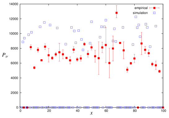
Figure 10: The resulting rent distribution along the Tozai-subway line obtained by the quasi-one-dimensional model. The correspondence between $x$-axis and the location of each subway station is explicitly given as follows: Bus-center mae ($x=86$), $\bar{O}$dori ($x=76$), Nishi 11-Choume ($x=54$), Nishi 18-Choume ($x=36$), Maruyama Kouen ($x=22$), and Nishi 28-Choume ($x=11$).

6.2 Probabilistic search depending on the location of office

Some of buyers might search their housing locations by taking into account the place of their office. Here we consider the attractiveness $B_{k,i}(\bm{X},t)$ of office location $\bm{X}$ for $i$ ranking $k$ at time $t$. Namely, we should remember that the attractiveness for the place to live is updated as

$$A_{k}(\bm{X},t+1)=A_{k}(\bm{X},t)+\omega(A^{0}(\bm{X})-A_{k}(\bm{X},t))+\epsilon\sum_{k^{{}^{\prime}}\geq k}v_{k}^{{}^{\prime}}(\bm{X},t)$$ (20)

depending on the intrinsic attractiveness of place to live, whereas the attractiveness of the place $\bm{X}$ for agent $i$ of ranking $k$ who takes into account the location of their office place $\bm{Y}_{k,i}$ is also defined accordingly and it is governed by

$$B_{k,i}(\bm{X},t+1)=B_{k,i}(\bm{X},t)+\overline{\omega}(B_{k,i}^{0}(|\bm{X}-\bm{Y}_{k,i}|)-B_{k,i}(\bm{X},t))+\overline{\epsilon}\sum_{k^{{}^{\prime}}\geq k}v_{k^{{}^{\prime}}}(\bm{X},t)$$ (21)

where $B_{k,i}^{0}(|\bm{X}-\bm{Y}_{k,i}|)$ is ‘intrinsic attractiveness’ of the location $\bm{X}$ for the agent $i$ whose office is located at $\bm{Y}_{k,i}$ and it is given explicitly by

$$B_{k,i}^{0}(|\bm{X}-\bm{Y}_{k,i}|)=\frac{1}{\sqrt{2\pi}Q}{\exp}\left[-\frac{(\bm{X}-\bm{Y}_{k,i})^{2}}{2\pi Q^{2}}\right],$$ (22)

and $\overline{\omega},\overline{\epsilon}$ are parameters to be calibrated using the empirical data sets.

Then, agent $i$ looks for the candidates $\bm{X}_{A},\bm{X}_{B}$ to live according to the following probabilities

$$\pi_{k}^{(A)}(\bm{X},t) = \frac{1-{\exp}(-\lambda A_{k}(\bm{X},t))}{\sum_{\bm{X}^{{}^{\prime}}\in\Omega}\{1-{\exp}(-\lambda A_{k}(\bm{X}^{{}^{\prime}},t))\}}$$ (23)

$$\pi_{k,i}^{(B)}(\bm{X},t) = \frac{1-{\exp}(-\lambda B_{k,i}(\bm{X},t))}{\sum_{\bm{X}^{{}^{\prime}}\in\Omega}\{1-{\exp}(-\lambda B_{k,i}(\bm{X}^{{}^{\prime}},t))\}}$$ (24)

If the both $\bm{X}_{A},\bm{X}_{B}$ are approved, transaction price for each place is given by

$$P_{\rm tr}^{(A)} = (1-\beta)P_{k^{{}^{\prime}}}(\bm{X}_{A})+\beta P_{k}$$ (25)

$$P_{\rm tr}^{(B)} = (1-\beta)P_{k^{{}^{\prime}}}(\bm{X}_{B})+\beta P_{k}$$ (26)

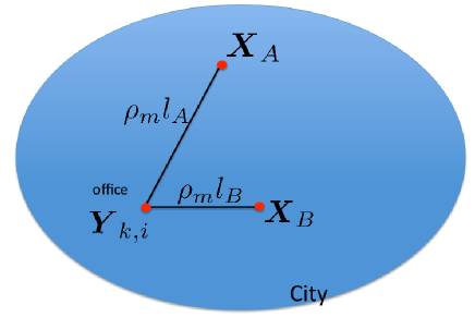
Figure 11: Each buyer decides the final location $\bm{X}_{F}={\arg\min}\{P_{\rm tr}^{(A)}+\rho_{m}l_{A},,P_{\rm tr}^{(B)}+\rho_{m}l_{B}\},F=\{A,B\}$.

The finial decision $\bm{X}_{F}$ is

$$\bm{X}_{F}={\arg\min}\{P_{\rm tr}^{(A)}+\rho_{m}l_{A},,P_{\rm tr}^{(B)}+\rho_{m}l_{B}\},\,F=\{A,B\}$$ (27)

where $\rho_{m}l_{A},\rho_{m}l_{B}$ are travel costs between $\bm{X}_{A},\bm{X}_{B}$ and office (see Fig. 11).

Therefore, the agents might prefer relatively closer place to the office to the attractive place to live when the distance between the attractive place to live and the office is too far for agents to manage the cost by the commuting allowance.

- (1) L. Gauvin, A. Vignes and J.-P. Nadal, Modeling urban housing market dynamics: can the socio-spatial segregation preserve some social diversity?, Journal of Economic Dynamics and Controls 37, Issue 7, pp. 1300-1321 (2013).
- (2) M. Ballerini, N. Cabibbo, R. Candelier, A. Cavagna, E. Cisbani, I. Giardina, V. Lecomte, A. Orlandi, G. Parisi, A. Procaccini, M. Viale and V. Zdravkovic, Interaction Rulling Animal Collective Behaviour Depends on Topological rather than Metric Distance, Evidence from a Field Study, Proceedings of the National Academy of Sciences USA 105, pp.1232-1237 (2008).
- (3) C.W. Reynolds, Flocks, Herds, and Schools: A Distributed Behavioral Model, Computer Graphics 21, 25 (1987).
- (4) M. Makiguchi and J. Inoue, Numerical Study on the Emergence of Anisotropy in Artificial Flocks: A BOIDS Modelling and Simulations of Empirical Findings, Proceedings of the Operational Research Society Simulation Workshop 2010 (SW10), CD-ROM, pp. 96-102 (the preprint version, arxiv:1004 3837) (2010). See also M. Makiguchi and J. Inoue, Emergence of Anisotropy in Flock Simulations and Its Computational Analysis, Transactions of the Society of Instrument and Control Engineers 46, No. 11, pp. 666-675 (2010) (in Japanese).
- (5) R. Olfati-Saber, Flocking for Multi-Agent Dynamic Systems: Algorithms and Theory, IEEE Trans. on Automatic control 51, No. 3, pp.401-420 (2006).
- (6) M. Fujita, P. Krugman and A.J. Venables, The Spatial Economy: Cities, Regions, and International Trade, The MIT Press (2001).
- (7) H. Chen and J. Inoue, Dynamics of probabilistic labor markets: statistical physics perspective, Lecture Notes in Economics and Mathematical Systems 662, pp. 53-64, “Managing Market Complexity”, Springer (2012), H. Chen and J. Inoue, Statistical Mechanics of Labor Markets, Econophysics of systemic risk and network dynamics, New Economic Windows, Springer-Verlag (Italy-Milan), pp. 157-171 (2013), H. Chen and J. Inoue, Learning curve for collective behavior of zero-intelligence agents in successive job-hunting processes with a diversity of Jaynes-Shannon’s MaxEnt principle, Evolutionary and Institutional Economics Review 10, No. 1, pp. 55-80 (2013).
- (8) http://www.souba-adpark.jp/
- (9) http://en.wikipedia.org/wiki/Sapporo
- (10) http://rnk.uub.jp/
- (11) http://www.homes.co.jp/