Bivariate Shepard-Bernoulli operators

Abstract.

In this paper we extend the Shepard-Bernoulli operators introduced in [6] to the bivariate case. These new interpolation operators are realized by using local support basis functions introduced in [23] instead of classical Shepard basis functions and the bivariate three point extension [13] of the generalized Taylor polynomial introduced  by F. Costabile in [11]. The new operators do not require either the use of special partitions of the node convex hull or special structured data as in [8]. We deeply study their approximation properties and provide an application to the scattered data interpolation problem; the numerical results show that this new approach is comparable with the other well known bivariate schemes QSHEP2D and CSHEP2D by Renka [34, 35].

1. The problem

Let $\mathcal{N}=\left\{\boldsymbol{x}_{1},...,\boldsymbol{x}_{N}\right\}$ be a set of $N$ distinct points (called nodes or sample points) of $\mathbb{R}^{s},s\in\mathbb{N}$, and let $f$ be a function defined on a domain $D$ containing $\mathcal{N}$. The classical Shepard operators (first introduced in [37] in the particular case $s=2$) are defined by

(1.1) $$S_{N,\mu}\left[f\right]\left(\boldsymbol{x}\right):={\displaystyle\sum\limits_{i=1}^{N}}A_{\mu,i}\left(\boldsymbol{x}\right)f\left(\boldsymbol{x}_{i}\right),\quad\mu>0,$$

where the weight functions $A_{\mu,i}\left(\boldsymbol{x}\right)$ in barycentric form are

(1.2) $$A_{\mu,i}\left(\boldsymbol{x}\right):=\frac{\left|\boldsymbol{x}-\boldsymbol{x}_{i}\right|^{-\mu}}{{\displaystyle\sum\limits_{k=1}^{N}}\left|\boldsymbol{x}-\boldsymbol{x}_{k}\right|^{-\mu}}$$

and $\left|\cdot\right|$ denotes the Euclidean norm in $\mathbb{R}^{s}$. The interpolation operator $S_{N,\mu}\left[\cdot\right]$ is stable, in the sense that

$$\min_{i}f\left(\boldsymbol{x}_{i}\right)\leq S_{N,\mu}\left[f\right]\left(\boldsymbol{x}\right)\leq\max_{i}f\left(\boldsymbol{x}_{i}\right)$$

but for $\mu>1$ the interpolating function $S_{N,\mu}\left[f\right]\left(\boldsymbol{x}\right)$ has flat spots in the neighborhood of all data points. Moreover, the degree of exactness of the operator $S_{N,\mu}\left[\cdot\right]$ is $0$, i.e. if it is restricted to the polynomial space $\mathcal{P}_{\boldsymbol{x}}^{m}:=\left\{p:\deg\left(p\right)\leq m\right\}$, then $\left.S_{N,\mu}\left[\cdot\right]\right|_{\mathcal{P}_{\boldsymbol{x}}^{m}}=Id_{\mathcal{P}_{\boldsymbol{x}}^{m}}$ (the identity function on $\mathcal{P}_{\boldsymbol{x}}^{m}$) only for $m=0$.

These drawbacks, in particular, can be avoided by replacing each value $f\left(\boldsymbol{x}_{i}\right)$ in (1.1) with an interpolation operator in $\boldsymbol{x}_{i}$, applied to $f$, with a degree of exactness $m>0$ [6]. In addition, to make the Shepard method a local one, according to [23] we multiply Euclidean distances $\left|\boldsymbol{x}-\boldsymbol{x}_{j}\right|,j=1,\ldots,N$ in (1.2) by Franke-Little weights [27]

$$\left(1-\frac{\left|\boldsymbol{x}-\boldsymbol{x}_{j}\right|}{R_{w_{j}}}\right)_{+}^{\mu},\text{ }R_{w_{j}}>0\text{ for each }j=1,\ldots,N$$

where $(\cdot)_{+}$ is the positive part of the argument. As a result, functions $A_{\mu,i}\left(\boldsymbol{x}\right)$ are replaced by compact support functions $\widetilde{W}_{\mu,i}\left(\boldsymbol{x}\right),$ $i=1,\ldots,N$ defined as follows:

(1.3) $$\widetilde{W}_{\mu,i}\left(\boldsymbol{x}\right):=\dfrac{W_{\mu,i}\left(\boldsymbol{x}\right)}{\sum\limits_{k=1}^{N}W_{\mu,k}\left(\boldsymbol{x}\right)}$$

where

$$W_{\mu,i}\left(\boldsymbol{x}\right):=\left(\frac{1}{\left|\boldsymbol{x}-\boldsymbol{x}_{i}\right|}-\frac{1}{R_{w_{i}}}\right)_{+}^{\mu},$$

and $R_{w_{i}}$ is the radius of influence about node $\boldsymbol{x}_{i}$: in practice $R_{w_{i}}$ is taken to be just large enough to include $N_{w}$ nodes in the open ball $B\left(\boldsymbol{x}_{i},R_{w_{i}}\right)=\left\{\boldsymbol{x}\in\mathbb{R}^{s}:\left|\boldsymbol{x}-\boldsymbol{x}_{i}\right|<R_{w_{i}}\right\}$ [34].

More precisely, if $P\left[\cdot,\boldsymbol{x}_{i}\right]$ denotes an interpolation operator in $\boldsymbol{x}_{i}$ based on data in the ball $B\left(\boldsymbol{x}_{i},R_{w_{i}}\right)$, $i=1,\dots,N$, the local combined Shepard operators are then defined as follows:

(1.4) $$\widetilde{S}_{N,\mu}P[f](\boldsymbol{x}):={\displaystyle\sum\limits_{i=1}^{N}}\widetilde{W}_{\mu,i}\left(\boldsymbol{x}\right)P[f,\boldsymbol{x}_{i}]\left(\boldsymbol{x}\right).$$

We emphasize that weight functions $\widetilde{W}_{\mu,i}\left(\boldsymbol{x}\right)$ have the same basic properties as weight functions $A_{\mu,i}\left(\boldsymbol{x}\right)$, but the value of the improved Shepard operator (1.4) at a point $\boldsymbol{x}\in D$ is influenced only by values $\widetilde{W}_{\mu,i}\left(\boldsymbol{x}\right)P[f,\boldsymbol{x}_{i}]\left(\boldsymbol{x}\right)$ with $\boldsymbol{x}_{i}\in\mathcal{N}_{\boldsymbol{x}}:=\left\{\boldsymbol{x}_{k}\in\mathcal{N}:\left|\boldsymbol{x}-\boldsymbol{x}_{k}\right|<R_{w_{k}}\right\}$.

Starting from Shepard himself various combinations have been proposed in order to improve the approximation properties of the Shepard operators (see, for example, [10, 21]): Shepard-Bernoulli operators introduced recently in [6] represent a further attempt. These univariate operators are obtained by replacing each value $f\left(x_{i}\right)$ in (1.1) with the generalized Taylor polynomial $P_{m}[f,x_{i},x_{i+1}](x)$, proposed by F. Costabile in [11]. In [6] the rate of convergence of the Shepard-Bernoulli operators is studied in depth and numerical examples demonstrate the accuracy of the proposed combination in special situations, in particular, when it is applied to the problem of interpolating the discrete solutions of initial value problems for ordinary differential equations. In the conclusion of [6] the possibility of extending the Shepard-Bernoulli operator to higher dimension was hypothesized by using the expansions studied in [12, 13].

In 2007 T. Catinas [8] combined classic Shepard operators with the tensorial extension of the generalized Taylor polynomial discussed in [12]. The resulting combination has separated degree of exactness $m$ with respect to $x$ and $n$ with respect to $y$ when applied to sufficiently smooth functions in the convex hull of data; it uses $N+2\left(N-1\right)$ specially structured three-dimensional data (in the situation depicted in [8] each point of $\mathcal{N}$ is the vertex of a rectangle with vertices in $\mathcal{N}$) but, on account of the nature of the polynomial, it interpolates only $N$ of them. The numerical results provided in the paper, on some of the test functions provided in [32, 36], show that the accuracy of the operator can be improved by using compact support basis functions $\widetilde{W}_{\mu,i}$ instead of the global basis functions $A_{\mu,i}$.

In this paper we extend the Shepard-Bernoulli operators to the bivariate case using local basis functions $\widetilde{W}_{\mu,i}$ and the three point interpolation polynomials discussed in [13] and introduce a new combination which interpolates on all data used for its definition. We do this by associating to each sample point $\boldsymbol{x}_{i}$ a triangle with a vertex in it and other two vertices in $B\left(\boldsymbol{x}_{i},R_{w_{i}}\right)$; the association is done in order to reduce the error of the three point interpolation polynomial based on the three vertices of the triangle. For fixed values of $N_{w}$ [34] this choice allows us to reduce the error of the proposed combination. As a consequence, the resulting operator not only interpolates at each sample point and increases by $1$ the degree of exactness of the Shepard-Taylor operator [21] which uses the same data, but also improves its accuracy.

The paper is organized as follows. We start section 2 by briefly recalling the definition of the generalized Taylor polynomial. Then we deal with the extension $P_{m}^{\left[\Delta_{2}\left(V_{1},V_{2},V_{3}\right);V_{1}\right]}[f]$ of the generalized Taylor polynomial to a generic simplex $\Delta_{2}\left(V_{1},V_{2},V_{3}\right)$ of vertices $V_{1},V_{2},V_{3}\in D$. In particular we provide new results concerning: error of approximation, limit behaviour and interpolation conditions of the given extension. In section 3 we use these results to define the bivariate Shepard-Bernoulli operators and to study their remainder terms and rate of convergence. In section 4 we apply the bivariate Shepard-Bernoulli operators to the scattered data interpolation problem. The numerical results on some commonly used test functions for scattered data approximation [32, 36] show that the bivariate interpolation scheme proposed here is comparable well with the better known operators QSHEP2D [34] and CSHEP2D [35]. Finally, in section 5 we draw conclusions.

2. Further remarks on the generalized Taylor polynomial.

2.1. The univariate expansion in Bernoulli polynomials.

The generalized Taylor polynomial [11] is an expansion in Bernoulli polynomials, i.e. in polynomials defined recursively by means of the following relations [11, 28]

(2.1) $$\left\{\begin{array}[c]{ll}B_{0}\left(x\right)=1,&\\ B_{n}^{\prime}\left(x\right)=nB_{n-1}\left(x\right),&n\geq 1,\\ {\displaystyle\int\limits_{0}^{1}}B_{n}\left(x\right)dx=0,&n\geq 1.\end{array}\right.$$

For functions in the class $C^{m}\left(\left[a,b\right]\right),\ a,b\in\mathbb{R},\ a<b$, this expansion is realized by the equation

(2.2) $$f\left(x\right)=P_{m}[f,a,b](x)+R_{m}\left[f,a,b\right](x),\quad x\in\left[a,b\right],$$

the polynomial approximant is defined by

(2.3) $$P_{m}[f,a,b](x)=f\left(a\right)+{\displaystyle\sum\limits_{k=1}^{m}}\frac{S_{k}\left(\dfrac{x-a}{h}\right)}{k!}h^{k-1}\left(f^{(k-1)}\left(b\right)-f^{\left(k-1\right)}\left(a\right)\right)\$$

and the remainder term is

(2.4) $$R_{m}\left[f,a,b\right](x)=\frac{h^{m-1}}{m!}{\displaystyle\int\limits_{a}^{b}}f^{\left(m\right)}\left(t\right)\left(B_{m}\left(\frac{b-t}{h}\right)-B_{m}\left(\frac{\left(x-t\right)-\left[x-t\right]}{h}\right)\right)dt,$$

where we have set $S_{k}\left(x\right)=B_{k}\left(x\right)-B_{k}$, $B_{k}=B_{k}\left(0\right)$ and we have denoted by $\left[\cdot\right]$ the integer part of the argument and $h=b-a$. The polynomial $P_{m}[f,a,b]$ can be extended in a natural way to the whole real line; in this case Peano’s kernel theorem [20, p. 70] provides an integral expression for the remainder (2.4) [6]. The main properties of the generalized Taylor polynomial have been extensively studied in [6, 11].

2.2. The bivariate extension.

In [13] the univariate expansion (2.2) has been extended to a bivariate expansion for functions of class $C^{m}$ in the standard simplex $\Delta_{2}=\left\{\left(x,y\right)\in\mathbb{R}^{2}:x\geq 0,y\geq 0,x+y\leq 1\right\}$ which interpolates at the vertices of the simplex and it is exact in $\mathcal{P}_{\boldsymbol{x}}^{m}$. As mentioned in [13], this expansion can be generalized to a generic simplex of $\mathbb{R}^{2}$ by means of a linear isomorphism. In this paper we require this general expansion and, in order to formalize it, let us denote by $\mathbb{Z}_{+}^{2}$ the set of all pairs with non-negative integer components in the euclidean space $\mathbb{R}^{2}$. For $\beta=\left(\beta_{1},\beta_{2}\right)\in\mathbb{Z}_{+}^{2}$, we use the notations $\left|\beta\right|=\beta_{1}+\beta_{2}$, $\beta!=\beta_{1}!\beta_{2}!$ and $\beta\leq\alpha$ if and only if $\beta_{i}\leq\alpha_{i}$ for all $i=1,2$. Moreover, we assume that $D$ is a compact convex domain and $V_{1},V_{2},V_{3}\in D$. To fix the ideas we set $V_{1}=(x_{1,}y_{1}),~{}V_{2}=\left(x_{2},y_{2}\right),~{}V_{3}=\left(x_{3},y_{3}\right)$. We denote by $\Delta_{2}\left(V_{1},V_{2},V_{3}\right)$ the simplex of vertices $V_{1},V_{2},V_{3}$, i.e. the convex hull of the set $\left\{V_{1},V_{2},V_{3}\right\}$. The baricentric coordinates $\left(\lambda_{1}\left(\boldsymbol{x}\right),\lambda_{2}\left(\boldsymbol{x}\right),\lambda_{3}\left(\boldsymbol{x}\right)\right)$, of a generic point $\boldsymbol{x}=\left(x,y\right)$$\in\mathbb{R}^{2}$, relative to the simplex $\Delta_{2}\left(V_{1},V_{2},V_{3}\right)$, are defined by

(2.5) $$\begin{array}[c]{ccc}\lambda_{1}\left(\boldsymbol{x}\right)=\dfrac{A\left(\boldsymbol{x},V_{2},V_{3}\right)}{A\left(V_{1},V_{2},V_{3}\right)},&\lambda_{2}\left(\boldsymbol{x}\right)=\dfrac{A\left(V_{1},\boldsymbol{x},V_{3}\right)}{A\left(V_{1},V_{2},V_{3}\right)},&\lambda_{3}\left(\boldsymbol{x}\right)=\dfrac{A\left(V_{1},V_{2},\boldsymbol{x}\right)}{A\left(V_{1},V_{2},V_{3}\right)}\end{array}$$

where $A\left(V_{1},V_{2},V_{3}\right)$ is the signed area of the simplex of vertices $V_{1},V_{2},V_{3}$

$$A\left(V_{1},V_{2},V_{3}\right)=\left|\begin{array}[c]{ccc}1&1&1\\ x_{1}&x_{2}&x_{3}\\ y_{1}&y_{2}&y_{3}\end{array}\right|.$$

If $f$ is a differentiable function, and $V_{i}$ and $V_{j}$ are two distinct vertices of the simplex $\Delta_{2}\left(V_{1},V_{2},V_{3}\right)$, the derivative of $f$ along the directed line segment from $V_{i}$ to $V_{j}$ (side of the simplex) at $\boldsymbol{x}$ is denoted by

(2.6) $$\begin{array}[c]{cc}D_{ij}f\left(\boldsymbol{x}\right):=\left(V_{i}-V_{j}\right)\cdot\nabla f\left(\boldsymbol{x}\right),&i,j=1,2,3,i\neq j,\end{array}$$

where $\cdot$ is the dot product and $\nabla f\left(\boldsymbol{x}\right)=\left(\dfrac{\partial f}{\partial x}\left(\boldsymbol{x}\right),\dfrac{\partial f}{\partial y}\left(\boldsymbol{x}\right)\right)$. The composition of derivatives along the directed sides of the simplex (2.6) are denoted by

(2.7) $$\begin{array}[c]{ccc}D_{1}^{\beta}=D_{21}^{\beta_{1}}D_{31}^{\beta_{2}},&D_{2}^{\beta}=D_{12}^{\beta_{1}}D_{32}^{\beta_{2}},&D_{3}^{\beta}=D_{13}^{\beta_{1}}D_{23}^{\beta_{2}}.\end{array}$$

The following theorem holds:

Theorem 2.1.

Let $f$ be a function of class $C^{m}\left(D\right)$. Then for each $\boldsymbol{x}\in\Delta_{2}\left(V_{1},V_{2},V_{3}\right)$ we have

(2.8) $$f\left(\boldsymbol{x}\right)=P_{m}^{\left[\Delta_{2}\left(V_{1},V_{2},V_{3}\right);V_{1}\right]}[f](\boldsymbol{x})+R_{m}^{\left[\Delta_{2}\left(V_{1},V_{2},V_{3}\right);V_{1}\right]}\left[f\right]\left(\boldsymbol{x}\right)$$

where

(2.9) $$\begin{array}[t]{l}P_{m}^{\left[\Delta_{2}\left(V_{1},V_{2},V_{3}\right);V_{1}\right]}[f](\boldsymbol{x})=f\left(V_{1}\right)\\ \quad\quad+{\displaystyle\sum\limits_{j=1}^{m}}\left(D_{1}^{\left(0,j-1\right)}f\left(V_{3}\right)-D_{1}^{\left(0,j-1\right)}f\left(V_{1}\right)\right)\dfrac{S_{j}\left(\lambda_{2}+\lambda_{3}\right)}{j!}\\ \quad\quad+{\displaystyle\sum\limits_{i=1}^{m}}{\displaystyle\sum\limits_{j=1}^{m-i+1}}\left(\left(-1\right)^{i+j}\left(D_{2}^{\left(j-1,i-1\right)}f\left(V_{2}\right)-D_{2}^{\left(j-1,i-1\right)}f\left(V_{1}\right)\right)\right.\\ \quad\quad\left.+\left(-1\right)^{j}\left(D_{3}^{\left(j-1,i-1\right)}f\left(V_{3}\right)-D_{3}^{\left(j-1,i-1\right)}f\left(V_{1}\right)\right)\right)\\ \quad\quad\times\dfrac{\left(\lambda_{2}+\lambda_{3}\right)^{i-1}S_{i}\left(\frac{\lambda_{2}}{\lambda_{2}+\lambda_{3}}\right)}{i!}\dfrac{S_{j}\left(\lambda_{2}+\lambda_{3}\right)}{j!},\end{array}$$

and $R_{m}^{\left[\Delta_{2}\left(V_{1},V_{2},V_{3}\right);V_{1}\right]}\left[f\right]\left(\boldsymbol{x}\right)$ is the remainder term.

Proof sketch.

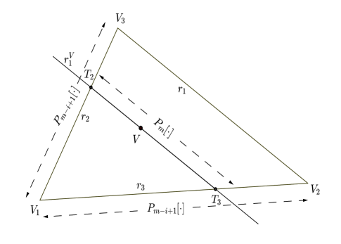
Rather than obtaining expansion (2.9) by using a linear transformation which maps points $\left(0,0\right),\left(1,0\right),\left(0,1\right)$ in points $\left(x_{1},y_{1}\right),\left(x_{2},y_{2}\right),\left(x_{3},y_{3}\right)$ respectively, we proceed by adapting, in this general case, the extension technique to the simplex specially developed in [13, 14] for expansions in Bernoulli and Lidstone polynomials (see also [18] for extensions of asymmetric expansions). We denote by $r_{1}~{}$the line through $V_{2},V_{3}$, by $r_{2}$ the line through $V_{1},V_{3}$ and by $r_{3}$ the line through $V_{1},V_{2}$. Let $V=\left(x,y\right)\in\Delta_{2}\left(V_{1},V_{2},V_{3}\right)$ be an interior point. We denote by $r_{1}^{V}$ the line through $V$ parallel to the line $r_{1}$ and by $T_{2}\left(x,y\right)=\left(x-\lambda_{2}h_{1},y-\lambda_{2}k_{1}\right),T_{3}\left(x,y\right)=\left(x+\lambda_{3}h_{1},y+\lambda_{3}k_{1}\right)$ the intersection points between $r_{1}^{V}$ and $r_{2},r_{3}$, respectively, where $\left(h_{1},k_{1}\right)=V_{2}-V_{3}$. We assign point $V$ to the line segment $S\left(x,y\right)=\left[T_{2},T_{3}\right]$ parameterized by

$$\left\{\begin{array}[c]{cc}\begin{array}[c]{c}x\left(\lambda\right)=x-\lambda_{2}h_{1}+\lambda\left(\lambda_{2}+\lambda_{3}\right)h_{1}\\ y\left(\lambda\right)=y-\lambda_{2}k_{1}+\lambda\left(\lambda_{2}+\lambda_{3}\right)k_{1}\end{array},&\lambda\in\left[0,1\right].\end{array}\right.$$

The restriction of $f$ to $S$ is the univariate function $f\left(x\left(\lambda\right),y\left(\lambda\right)\right)$ in $\left[0,1\right]$ and we expand it by generalized Taylor expansion (2.2). In this expansion we replace parameter $\lambda$ by the value $\frac{\lambda_{2}}{\lambda_{2}+\lambda_{3}}$ which corresponds to point $V$. This results in an expansion in terms of the values at $T_{2},T_{3}$ of $f$ and its derivatives in direction of the side $V_{2},V_{3}$. We reach the vertices of the simplex $\Delta_{2}\left(V_{1},V_{2},V_{3}\right)$ by assigning points $T_{2},T_{3}$ to the segments with end points $V_{1},V_{3}$ and $V_{1},V_{2}$ respectively and by repeated use of the expansion (2.2) on $f$ and its directional derivatives (see fig. 1).

Figure 1. Let $V=\left(x,y\right)\in\Delta_{2}\left(V_{1},V_{2},V_{3}\right)$. By assigning this point to the segment with end-points $T_{2},T_{3}$ we expand $f$ along this segment by generalized Taylor expansion; the vertices of the simplex are then reached by a repeated use of expansion (2.2) with respect to the points $V_{1},V_{3}$ and $V_{1},V_{2}$ on $f$ and its directional derivatives.

∎

If $\boldsymbol{x}\in\Delta_{2}\left(V_{1},V_{2},V_{3}\right)$ an expression for the remainder $R_{m}^{\left[\Delta_{2}\left(V_{1},V_{2},V_{3}\right);V_{1}\right]}\left[f\right]\left(\boldsymbol{x}\right)$ can be obtained by a repeated use of (2.4) as in [13]. If $\boldsymbol{x}\in D$ the following Theorem provides an expression for $R_{m}^{\left[\Delta_{2}\left(V_{1},V_{2},V_{3}\right);V_{1}\right]}\left[f\right]\left(\boldsymbol{x}\right)$ under only slightly stronger hypothesis on $f$. More precisely, we consider the class $C^{m,1}\left(D\right)$ of functions $f\in C^{m}\left(D\right)$ [39] with partial derivatives $\frac{\partial^{m}f}{\partial x^{m-j}\partial y^{j}}$ Lipschitz-continuous in $D$ for each $j=0,\dots,m$ and we set [21]

(2.10) $$\left|f\right|_{m,1}=\sup_{j=0,\dots,m}\left\{\frac{\left|\frac{\partial^{m}f}{\partial x^{m-j}\partial y^{j}}\left(\boldsymbol{u}_{1}\right)-\frac{\partial^{m}f}{\partial x^{m-j}\partial y^{j}}\left(\boldsymbol{u}_{2}\right)\right|}{\left|\boldsymbol{u}_{1}-\boldsymbol{u}_{2}\right|},\boldsymbol{u}_{1}\neq\boldsymbol{u}_{2}\text{ in }D\right\}.$$

Theorem 2.2.

Let $f$ be a function of class $C^{m,1}\left(D\right)$. Then for each $\boldsymbol{x}\in D$ we have

(2.11) $$P_{m}^{\left[\Delta_{2}\left(V_{1},V_{2},V_{3}\right);V_{1}\right]}[f](\boldsymbol{x})=T_{m}\left[f,V_{1}\right]\left(\boldsymbol{x}\right)+\delta_{m}^{\left[\Delta_{2}\left(V_{1},V_{2},V_{3}\right);V_{1}\right]}[f](\boldsymbol{x})$$

where $T_{m}\left[f,V_{1}\right]\left(\boldsymbol{x}\right)$ is the Taylor polynomial of order $m$ for $f$ at $V_{1}$ [1, Ch. 1] and

(2.12) $$\begin{array}[t]{l}\delta_{m}^{\left[\Delta_{2}\left(V_{1},V_{2},V_{3}\right);V_{1}\right]}[f](\boldsymbol{x})=\\ \quad{\displaystyle\sum\limits_{j=1}^{m}}{\displaystyle\int_{0}^{1}}\frac{D_{31}^{m-j+2}D_{1}^{\left(0,j-1\right)}f\left(V_{1}+t\left(V_{3}-V_{1}\right)\right)\left(1-t\right)^{m-j+1}}{\left(m-j+1\right)!}dt\dfrac{S_{j}\left(\lambda_{2}+\lambda_{3}\right)}{j!}\\ \quad+{\displaystyle\sum\limits_{i=1}^{m}}{\displaystyle\sum\limits_{j=1}^{m-i+1}}\left(\left(-1\right)^{i+j}{\displaystyle\int_{0}^{1}}\frac{D_{21}^{m-j-i+3}D_{2}^{\left(j-1,i-1\right)}f\left(V_{1}+t\left(V_{2}-V_{1}\right)\right)\left(1-t\right)^{m-j-i+2}}{(m-j-i+2)!}dt\right.\\ \quad+\left.\left(-1\right)^{j}{\displaystyle\int_{0}^{1}}\frac{D_{31}^{m-j-i+3}D_{3}^{\left(j-1,i-1\right)}f\left(V_{1}+t\left(V_{3}-V_{1}\right)\right)\left(1-t\right)^{m-j-i+2}}{(m-j-i+2)!}dt\right)\\ \quad\times\dfrac{\left(\lambda_{2}+\lambda_{3}\right)^{i-1}S_{i}\left(\frac{\lambda_{2}}{\lambda_{2}+\lambda_{3}}\right)}{i!}\dfrac{S_{j}\left(\lambda_{2}+\lambda_{3}\right)}{j!}.\end{array}$$

Proof.

By applying the Taylor theorem with integral remainder [2, Ch. 7] to all derivative differences in (2.9) we find

$$P_{m}^{\left[\Delta_{2}\left(V_{1},V_{2},V_{3}\right);V_{1}\right]}[f](\boldsymbol{x})=T_{m}\left[f,V_{1}\right]\left(\boldsymbol{x}\right)+\delta_{m}^{\left[\Delta_{2}\left(V_{1},V_{2},V_{3}\right);V_{1}\right]}[f](\boldsymbol{x})$$

where $\delta_{m}^{\left[\Delta_{2}\left(V_{1},V_{2},V_{3}\right);V_{1}\right]}[f](\boldsymbol{x})$ is as in (2.12) and

$$\begin{array}[c]{l}\widetilde{T}_{m}[f,V_{1}](\boldsymbol{x}):=f\left(V_{1}\right)+{\displaystyle\sum\limits_{j=1}^{m}}{\displaystyle\sum\limits_{k=1}^{m-j+1}}\dfrac{1}{k!}D_{1}^{\left(0,k+j-1\right)}f\left(V_{1}\right)\dfrac{S_{j}\left(\lambda_{2}+\lambda_{3}\right)}{j!}\\ \quad+{\displaystyle\sum\limits_{i=1}^{m}}{\displaystyle\sum\limits_{j=1}^{m-i+1}}{\displaystyle\sum\limits_{k=1}^{m-i-j+2}}\dfrac{1}{k!}\left(\left(-1\right)^{i+j+k}D_{2}^{\left(j-1+k,i-1\right)}f\left(V_{1}\right)+\left(-1\right)^{j+k}D_{3}^{\left(j-1+k,i-1\right)}f\left(V_{1}\right)\right)\\ \quad\times\dfrac{\left(\lambda_{2}+\lambda_{3}\right)^{i-1}S_{i}\left(\frac{\lambda_{2}}{\lambda_{2}+\lambda_{3}}\right)}{i!}\dfrac{S_{j}\left(\lambda_{2}+\lambda_{3}\right)}{j!}.\end{array}$$

Since $\delta_{m}^{\left[\Delta_{2}\left(V_{1},V_{2},V_{3}\right);V_{1}\right]}[f](\boldsymbol{x})\equiv 0$ for each $f\in\mathcal{P}_{\boldsymbol{x}}^{m}$ and $\operatorname{dex}\left(P_{m}^{\left[\Delta_{2}\left(V_{1},V_{2},V_{3}\right);V_{1}\right]}\left[\cdot\right]\right)=m$, the polynomial operator $\widetilde{T}_{m}\left[\cdot,V_{1}\right]$ reproduces exactly polynomials up to the degree $m$. For this reason we can affirm that $\widetilde{T}_{m}\left[f,V_{1}\right]$ is the $m$-th order Taylor polynomial $T_{m}\left[f,V_{1}\right]$ for $f$ centered at $V_{1}$

(2.13) $$T_{m}\left[f,V_{1}\right]\left(\boldsymbol{x}\right):=\sum\limits_{\begin{subarray}{c}\left|\alpha\right|\leq m\\ \alpha\in\mathbb{N}_{0}^{2}\end{subarray}}\frac{1}{\alpha!}\frac{\partial^{\left|\alpha\right|}f}{\partial x^{\alpha_{1}}\partial y^{\alpha_{2}}}\left(V_{1}\right)\left(x-x_{1}\right)^{\alpha_{1}}\left(y-y_{1}\right)^{\alpha_{2}}.$$

In fact, $\widetilde{T}_{m}\left[f,V_{1}\right]$ can be expressed, after some computation and rearrangement, in terms of some partial derivatives of $f$ up to the order $m$ at a point $V_{1}\in D$

$$\widetilde{T}_{m}\left[f,V_{1}\right]\left(\boldsymbol{x}\right)=\sum\limits_{\begin{subarray}{c}\left|\alpha\right|\leq m\\ \alpha\in\mathbb{N}_{0}^{2}\end{subarray}}\frac{\partial^{\left|\alpha\right|}f}{\partial x^{\alpha_{1}}\partial y^{\alpha_{2}}}\left(V_{1}\right)p_{\alpha}\left(\boldsymbol{x}\right),$$

where $p_{\alpha}\left(\boldsymbol{x}\right)$ are polynomials of degree at most $m$. Since $\widetilde{T}_{m}\left[f,V_{1}\right]=f$ for each $f\in\mathcal{P}_{\boldsymbol{x}}^{m}$ then $\left\{p_{\alpha}\left(\boldsymbol{x}\right):\left|\alpha\right|\leq m\right\}$ generates $\mathcal{P}_{\boldsymbol{x}}^{m}$, and therefore $p_{\alpha}\left(\boldsymbol{x}\right)\neq 0$ for each $\alpha$. Since $\widetilde{T}_{m}\left[\cdot,V_{1}\right]$ reproduces exactly all polynomials in $\mathcal{P}_{\boldsymbol{x}}^{m}$ it follows that

(2.14) $$\begin{array}[c]{cc}\widetilde{T}_{m}\left[T_{m}\left[f,V_{1}\right],V_{1}\right]\left(\boldsymbol{x}\right)=T_{m}\left[f,V_{1}\right]\left(\boldsymbol{x}\right),&\boldsymbol{x}\in D;\end{array}$$

on the other hand

(2.15) $$\begin{array}[c]{cc}\widetilde{T}_{m}\left[T_{m}\left[f,V_{1}\right],V_{1}\right]\left(\boldsymbol{x}\right)=\widetilde{T}_{m}\left[f,V_{1}\right]\left(\boldsymbol{x}\right),&\boldsymbol{x}\in D,\end{array}$$

since for each $\alpha$, such that $\left|\alpha\right|\leq m$

$$\frac{\partial^{\left|\alpha\right|}T_{m}\left[f,V_{1}\right]}{\partial x^{\alpha_{1}}\partial y^{\alpha_{2}}}\left(V_{1}\right)=\frac{\partial^{\left|\alpha\right|}f}{\partial x^{\alpha_{1}}\partial y^{\alpha_{2}}}\left(V_{1}\right).$$

Therefore, by equaling the right hand side terms of (2.14) and (2.15) we get

$$\widetilde{T}_{m}\left[f,V_{1}\right]\left(\boldsymbol{x}\right)=T_{m}\left[f,V_{1}\right]\left(\boldsymbol{x}\right).$$

∎

Corollary 2.3.

In the hypothesis of Theorem 2.2 equation (2.8) extends to all $\boldsymbol{x}\in D$ by setting

(2.16) $$R_{m}^{\left[\Delta_{2}\left(V_{1},V_{2},V_{3}\right);V_{1}\right]}\left[f\right]\left(\boldsymbol{x}\right)=R_{m}^{T}\left[f,V_{1}\right]\left(x,y\right)\left(\boldsymbol{x}\right)-\delta_{m}^{\left[\Delta_{2}\left(V_{1},V_{2},V_{3}\right);V_{1}\right]}[f](\boldsymbol{x})$$

where $R_{m}^{T}\left[f,V_{1}\right]\left(\boldsymbol{x}\right)$ is the remainder in the Taylor expansion [1, Ch. 1].

We are now able to give a bound for the remainder (2.16). From here on, we shall use the notation $\left|\lambda\right|$ for the absolute value of the real number $\lambda$ and $\left\|v\right\|_{2}$ for the modulus of the vector $v\in\mathbb{R}^{2}$. We set:

(2.17) $$r=\max\left\{\left\|V_{1}-V_{2}\right\|_{2},\left\|V_{1}-V_{3}\right\|_{2},\left\|V_{2}-V_{3}\right\|_{2}\right\}\text{ }$$

and

(2.18) $$S^{-1}=A\left(V_{1},V_{2},V_{3}\right).$$

By settings (2.5) and by the Cauchy-Schwarz inequality, we get the following inequalities

(2.19) $$\begin{array}[t]{lll}\left|\lambda_{i}\right|&\leq rS\left\|\boldsymbol{x}-V_{1}\right\|_{2},&i=2,3,\end{array}$$

(2.20) $$\begin{array}[t]{ll}\left|\lambda_{2}+\lambda_{3}\right|&\leq rS\left\|\boldsymbol{x}-V_{1}\right\|_{2}\end{array}$$

and

(2.21) $$\begin{array}[c]{ccc}\left|\dfrac{\partial\lambda_{i}}{\partial x}\right|\leq rS,&\left|\dfrac{\partial\lambda_{i}}{\partial y}\right|\leq rS,&i=2,3.\end{array}$$

The following Lemma provides bounds for the derivatives of $f$ along the directed sides of the simplex (2.7).

Lemma 2.4.

Let $f\in C^{m,1}\left(D\right)$. The derivatives of $f$ along the directed sides of the simplex $\Delta_{2}\left(V_{1},V_{2},V_{3}\right)$ satisfy

(2.22) $$\begin{array}[c]{cccc}\left|D_{j}^{\beta}f\left(\boldsymbol{x}\right)\right|\leq 2^{\left|\beta\right|}r^{\left|\beta\right|}\left|f\right|_{\left|\beta\right|-1,1},&j=1,2,3&\left|\beta\right|=m+1,&\boldsymbol{x}\in D.\end{array}$$

Proof.

Let us consider the case $j=1$. By (2.7) and (2.6) we have

$$\begin{array}[c]{l}D_{1}^{\beta}f\left(\boldsymbol{x}\right)=D_{21}^{\beta_{1}}D_{31}^{\beta_{2}}f\left(\boldsymbol{x}\right)=\sum\limits_{i=0}^{\beta_{1}}\binom{\beta_{1}}{i}(x_{2}-x_{1})^{\beta_{1}-i}\left(y_{2}-y_{1}\right)^{i}\\ \quad\sum\limits_{j=0}^{\beta_{2}}\binom{\beta_{2}}{j}(x_{3}-x_{1})^{\beta_{2}-j}\left(y_{3}-y_{1}\right)^{j}\frac{\partial^{\left|\beta\right|}f\left(\boldsymbol{x}\right)}{\partial x^{\left|\beta\right|-i-j}\partial y^{i+j}}.\end{array}$$

Since $\left|\beta\right|\geq 1$, at least one between $\left|\beta\right|-i-j$ and $i+j$ is greater than or equal to $1$, $i=0,\dots,\beta_{1}$, $j=0,\dots,\beta_{2}$. If $\left|\beta\right|-i-j\geq 1$

$$\left|\frac{\partial^{\left|\beta\right|}f\left(\boldsymbol{x}\right)}{\partial x^{\left|\beta\right|-i-j}\partial y^{i+j}}\right|=\left|\lim_{h\rightarrow 0}\frac{\frac{\partial^{\left|\beta\right|-1}f\left(x+h,y\right)}{\partial x^{\left|\beta\right|-i-j-1}\partial y^{i+j}}-\frac{\partial^{\left|\beta\right|-1}f\left(x,y\right)}{\partial x^{\left|\beta\right|-i-j-1}\partial y^{i+j}}}{h}\right|\leq\left|f\right|_{\left|\beta\right|-1,1}$$

otherwise

$$\left|\frac{\partial^{\left|\beta\right|}f\left(\boldsymbol{x}\right)}{\partial x^{\left|\beta\right|-i-j}\partial y^{i+j}}\right|=\left|\lim_{h\rightarrow 0}\frac{\frac{\partial^{\left|\beta\right|-1}f\left(x,y+h\right)}{\partial x^{\left|\beta\right|-i-j}\partial y^{i+j-1}}-\frac{\partial^{\left|\beta\right|-1}f\left(x,y\right)}{\partial x^{\left|\beta\right|-i-j}\partial y^{i+j-1}}}{h}\right|\leq\left|f\right|_{\left|\beta\right|-1,1}$$

$i=0,\dots,\beta_{1}$, $j=0,\dots,\beta_{2}$. Therefore we have

$$\begin{array}[c]{l}\left|D_{1}^{\beta}f\left(\boldsymbol{x}\right)\right|=\left|\sum\limits_{i=0}^{\beta_{1}}\binom{\beta_{1}}{i}(x_{2}-x_{1})^{\beta_{1}-i}\left(y_{2}-y_{1}\right)^{i}\right.\\ \qquad\left.\sum\limits_{j=0}^{\beta_{2}}\binom{\beta_{2}}{j}(x_{3}-x_{1})^{\beta_{2}-j}\left(y_{3}-y_{1}\right)^{j}\frac{\partial^{\left|\beta\right|}f\left(\boldsymbol{x}\right)}{\partial x^{\left|\beta\right|-i-j}\partial y^{i+j}}\right|\\ \qquad\leq\sum\limits_{i=0}^{\beta_{1}}\binom{\beta_{1}}{i}\left|\left|x_{2}-x_{1}\right|\right|_{2}^{\beta_{1}-i}\left|\left|y_{2}-y_{1}\right|\right|_{2}^{i}\\ \qquad\sum\limits_{j=0}^{\beta_{2}}\binom{\beta_{2}}{j}\left|\left|x_{3}-x_{1}\right|\right|_{2}^{\beta_{2}-j}\left|\left|y_{3}-y_{1}\right|\right|_{2}^{j}\left|\frac{\partial^{\left|\beta\right|}f\left(\boldsymbol{x}\right)}{\partial x^{\left|\beta\right|-i-j}\partial y^{i+j}}\right|\\ \qquad\leq 2^{\left|\beta\right|}\left|\left|V_{2}-V_{1}\right|\right|_{2}^{\beta_{1}}\left|\left|V_{3}-V_{1}\right|\right|_{2}^{\beta_{2}}\left|f\right|_{\left|\beta\right|-1,1}\\ \qquad\leq 2^{\left|\beta\right|}r^{\left|\beta\right|}\left|f\right|_{\left|\beta\right|-1,1}.\end{array}$$

The cases $j=2,3$ are analogous. ∎

Now, we are able to prove the following Theorem.

Theorem 2.5.

Let $f$ be a function of class $C^{m,1}\left(D\right)$. Then for each $\boldsymbol{x}\in D$ we have the following bound for the derivative $\dfrac{\partial^{\alpha+\beta}\delta_{m}^{\left[\Delta_{2}\left(V_{1},V_{2},V_{3}\right);V_{1}\right]}\left[f\right]\left(\boldsymbol{x}\right)}{\partial x^{\alpha}\partial y^{\beta}}$ of the difference (2.12), for each $\alpha,\beta:$ $0\leq\alpha+\beta\leq m$

(2.23) $$\left|\dfrac{\partial^{\alpha+\beta}\delta_{m}^{\left[\Delta_{2}\left(V_{1},V_{2},V_{3}\right);V_{1}\right]}\left[f\right]\left(\boldsymbol{x}\right)}{\partial x^{\alpha}\partial y^{\beta}}\right|\leq\left|f\right|_{m,1}C_{\alpha,\beta}\left(m\right){\displaystyle\sum\limits_{l=\max\left\{1,\alpha+\beta\right\}}^{m}}r^{m+1-l}\left(r^{2}S\right)^{l}\left\|\boldsymbol{x}-V_{1}\right\|_{2}^{l-\left(\alpha+\beta\right)}$$

where $C_{\alpha,\beta}\left(m\right)$ is a constant independent of $f$ or $\boldsymbol{x}$ explicitly computable.

Proof.

From properties of Bernoulli polynomials [28], [17]

$$B_{n}\left(t\right)={\textstyle\sum\limits_{k=0}^{n}}\dbinom{n}{k}B_{k}t^{n-k},\quad n=0,1,2,\ldots$$

it follows that

(2.24) $$\begin{array}[t]{ll}S_{n}\left(t\right)&=B_{n}\left(t\right)-B_{n}\\ &={\textstyle\sum\limits_{k=0}^{n-1}}\dbinom{n}{k}B_{k}t^{n-k},\quad n=1,2,\ldots\end{array}$$

Moreover, we express the derivative $\dfrac{\partial^{\alpha+\beta}}{\partial x^{\alpha}\partial y^{\beta}}$ as a combination of derivatives along the directed line segments from $V_{2}$ to $V_{1}$ and from $V_{3}$ to $V_{1}$. In fact, from relations (2.6) we obtain

$$\begin{array}[c]{c}\frac{\partial}{\partial x}=\frac{\partial\lambda_{3}}{\partial x}D_{31}+\frac{\partial\lambda_{2}}{\partial x}D_{21},\\ \frac{\partial}{\partial y}=\frac{\partial\lambda_{3}}{\partial y}D_{31}+\frac{\partial\lambda_{2}}{\partial y}D_{21},\end{array}$$

and then

(2.25) $$\begin{array}[c]{c}\dfrac{\partial^{\alpha+\beta}\delta_{m}^{\left[\Delta_{2}\left(V_{1},V_{2},V_{3}\right);V_{1}\right]}\left[f\right]\left(\boldsymbol{x}\right)}{\partial x^{\alpha}\partial y^{\beta}}={\displaystyle\sum\limits_{p=0}^{\alpha}}{\displaystyle\sum\limits_{q=0}^{\beta}}\dbinom{\alpha}{p}\dbinom{\beta}{q}\left(\dfrac{\partial\lambda_{2}}{\partial x}\right)^{p}\left(\dfrac{\partial\lambda_{3}}{\partial x}\right)^{\alpha-p}\\ \times\left(\dfrac{\partial\lambda_{2}}{\partial y}\right)^{q}\left(\dfrac{\partial\lambda_{3}}{\partial y}\right)^{\beta-q}D_{21}^{p+q}D_{31}^{\alpha+\beta-p-q}\delta_{m}^{\left[\Delta_{2}\left(V_{1},V_{2},V_{3}\right);V_{1}\right]}\left[f\right]\left(\boldsymbol{x}\right).\end{array}$$

By taking the modulus of both sides of (2.25) and by using relations (2.21) we get

(2.26) $$\left|\dfrac{\partial^{\alpha+\beta}\delta_{m}^{\left[\Delta_{2}\left(V_{1},V_{2},V_{3}\right);V_{1}\right]}[f](\boldsymbol{x})}{\partial x^{\alpha}\partial y^{\beta}}\right|\leq{\displaystyle\sum\limits_{p=0}^{\alpha}}{\displaystyle\sum\limits_{q=0}^{\beta}}\dbinom{\alpha}{p}\dbinom{\beta}{q}\left(rS\right)^{\alpha+\beta}\left|D_{21}^{p+q}D_{31}^{\alpha+\beta-p-q}\delta_{m}^{\left[\Delta_{2}\left(V_{1},V_{2},V_{3}\right);V_{1}\right]}\left[f\right]\left(\boldsymbol{x}\right)\right|.$$

Therefore we need to calculate and to bound

(2.27) $$D_{21}^{\gamma_{1}}D_{31}^{\gamma_{2}}\delta_{m}^{\left[\Delta_{2}\left(V_{1},V_{2},V_{3}\right);V_{1}\right]}[f](\boldsymbol{x})$$

for each $\gamma_{1}:=p+q$, $\gamma_{2}:=\alpha+\beta-p-q$, $p=0,\dots,\alpha$;  $q=0,\dots,\beta$. In order to calculate (2.27) we substitute relations (2.24) in equation (2.12) and, by the Binomial Theorem, we get

(2.28) $$\begin{array}[t]{l}\delta_{m}^{\left[\Delta_{2}\left(V_{1},V_{2},V_{3}\right);V_{1}\right]}[f](\boldsymbol{x})=\\ \quad{\displaystyle\sum\limits_{j=1}^{m}}{\displaystyle\int_{0}^{1}}\frac{D_{31}^{m-j+2}D_{1}^{\left(0,j-1\right)}f\left(V_{1}+t\left(V_{3}-V_{1}\right)\right)\left(1-t\right)^{m-j+1}}{\left(m-j+1\right)!}dt\dfrac{{\textstyle\sum\limits_{k=0}^{j-1}}\binom{j}{k}B_{k}\left(\lambda_{2}+\lambda_{3}\right)^{j-k}}{j!}\\ \quad+{\displaystyle\sum\limits_{i=1}^{m}}{\displaystyle\sum\limits_{j=1}^{m-i+1}}\left(\left(-1\right)^{i+j}{\displaystyle\int_{0}^{1}}\frac{D_{21}^{m-j-i+3}D_{2}^{\left(j-1,i-1\right)}f\left(V_{1}+t\left(V_{2}-V_{1}\right)\right)\left(1-t\right)^{m-j-i+2}}{(m-j-i+2)!}dt\right.\\ \quad+\left.\left(-1\right)^{j}{\displaystyle\int_{0}^{1}}\frac{D_{31}^{m-j-i+3}D_{3}^{\left(j-1,i-1\right)}f\left(V_{1}+t\left(V_{3}-V_{1}\right)\right)\left(1-t\right)^{m-j-i+2}}{(m-j-i+2)!}dt\right)\\ \quad\times\dfrac{{\textstyle\sum\limits_{k=0}^{i-1}}\binom{i}{k}B_{k}}{i!}\dfrac{\sum\limits_{l=0}^{j-1}\binom{j}{l}B_{l}\sum\limits_{v=0}^{k+j-1-l}\binom{k+j-1-l}{v}\lambda_{2}^{i+j-1-l-v}\lambda_{3}^{v}}{j!}.\end{array}$$

The application of the operator $D_{21}^{\gamma_{1}}D_{31}^{\gamma_{2}}$ to $\delta_{m}^{\left[\Delta_{2}\left(V_{1},V_{2},V_{3}\right);V_{1}\right]}[f](\boldsymbol{x})$ causes the disappearing of some addenda on the right hand side of (2.28) therefore, to highlight this operation we make some changes of dummy index. Firstly we set $j-k=\kappa$ in the first sequence of sums ${\displaystyle\sum\limits_{j=1}^{m}}{\displaystyle\sum\limits_{k=1}^{j}}$ and $i+j-1=\iota$ in the second sequence of sums ${\displaystyle\sum\limits_{i=1}^{m}}{\displaystyle\sum\limits_{j=1}^{m-i+1}}$ and we get, by writing $k$ instead of $\kappa$ and $j$ instead of $\iota$

$$\begin{array}[t]{l}\delta_{m}^{\left[\Delta_{2}\left(V_{1},V_{2},V_{3}\right);V_{1}\right]}[f](\boldsymbol{x})=\\ \quad{\displaystyle\sum\limits_{j=1}^{m}}{\displaystyle\int_{0}^{1}}\frac{D_{31}^{m-j+2}D_{1}^{\left(0,j-1\right)}f\left(V_{1}+t\left(V_{3}-V_{1}\right)\right)\left(1-t\right)^{m-j+1}}{\left(m-j+1\right)!}dt\dfrac{{\textstyle\sum\limits_{k=1}^{j}}\binom{j}{j-\kappa}B_{j-k}\left(\lambda_{2}+\lambda_{3}\right)^{k}}{j!}\\ \quad{\displaystyle\sum\limits_{i=1}^{m}}{\displaystyle\sum\limits_{j=i}^{m}}\left(\left(-1\right)^{j+1}{\displaystyle\int_{0}^{1}}\frac{D_{21}^{m-j-1+3}D_{2}^{\left(j-i,i-1\right)}f\left(V_{1}+t\left(V_{2}-V_{1}\right)\right)\left(1-t\right)^{m-j+1}}{(m-j+1)!}dt\right.\\ \quad+\left.\left(-1\right)^{j-i+1}{\displaystyle\int_{0}^{1}}\frac{D_{31}^{m-j+2}D_{3}^{\left(j-i,i-1\right)}f\left(V_{1}+t\left(V_{3}-V_{1}\right)\right)\left(1-t\right)^{m-j+1}}{(m-j+1)!}dt\right)\\ \quad\times\dfrac{{\displaystyle\sum\limits_{k=0}^{i-1}}{\displaystyle\sum\limits_{l=0}^{j-i}}\binom{j-i+1}{l}B_{l}{\displaystyle\sum\limits_{v=0}^{k+j-i-l}}\binom{k+j-i-l}{v}\lambda_{2}^{j-l-v}\lambda_{3}^{v}}{i!(j-i+1)!}.\end{array}$$

Secondly we set $j-l=\lambda$ in the sequence of sums ${\displaystyle\sum\limits_{j=i}^{m}}{\displaystyle\sum\limits_{l=i}^{j}}$ and we get, by writing $l$ instead of $\lambda$,

$$\begin{array}[t]{l}\delta_{m}^{\left[\Delta_{2}\left(V_{1},V_{2},V_{3}\right);V_{1}\right]}[f](\boldsymbol{x})=\\ \quad{\displaystyle\sum\limits_{j=1}^{m}}{\displaystyle\int_{0}^{1}}\frac{D_{31}^{m-j+2}D_{1}^{\left(0,j-1\right)}f\left(V_{1}+t\left(V_{3}-V_{1}\right)\right)\left(1-t\right)^{m-j+1}}{\left(m-j+1\right)!}dt\dfrac{{\textstyle\sum\limits_{k=1}^{j}}\binom{j}{j-k}B_{j-k}\left(\lambda_{2}+\lambda_{3}\right)^{k}}{j!}\\ \quad+{\displaystyle\sum\limits_{i=1}^{m}}{\displaystyle\sum\limits_{j=i}^{m}}\left(\left(-1\right)^{j+1}{\displaystyle\int_{0}^{1}}\frac{D_{21}^{m-j-1+3}D_{2}^{\left(j-i,i-1\right)}f\left(V_{1}+t\left(V_{2}-V_{1}\right)\right)\left(1-t\right)^{m-j+1}}{(m-j+1)!}dt\right.\\ \quad+\left.\left(-1\right)^{j-i+1}{\displaystyle\int_{0}^{1}}\frac{D_{31}^{m-j+2}D_{3}^{\left(j-i,i-1\right)}f\left(V_{1}+t\left(V_{3}-V_{1}\right)\right)\left(1-t\right)^{m-j+1}}{(m-j+1)!}dt\right)\\ \quad\times\dfrac{\sum\limits_{k=0}^{i-1}\binom{i}{k}B_{k}\sum\limits_{l=i}^{j}\binom{j-i+1}{j-l}B_{j-l}\sum\limits_{v=0}^{k-i-l}\binom{k-i-l}{v}\lambda_{2}^{l-v}\lambda_{3}^{v}}{i!(j-i+1)!}.\end{array}$$

Thirdly we change the order of summations ${\displaystyle\sum\limits_{j=1}^{m}}{\displaystyle\sum\limits_{k=1}^{j}}={\displaystyle\sum\limits_{k=1}^{m}}{\displaystyle\sum\limits_{j=k}^{m}}$ and ${\displaystyle\sum\limits_{i=1}^{m}}{\displaystyle\sum\limits_{j=i}^{m}}{\displaystyle\sum\limits_{l=i}^{j}}={\displaystyle\sum\limits_{l=1}^{m}}{\displaystyle\sum\limits_{i=1}^{l}}{\displaystyle\sum\limits_{j=l}^{m}}$ and we get

$$\begin{array}[t]{l}\delta_{m}^{\left[\Delta_{2}\left(V_{1},V_{2},V_{3}\right);V_{1}\right]}[f](\boldsymbol{x})=\\ \quad{\displaystyle\sum\limits_{k=1}^{m}}{\displaystyle\sum\limits_{j=k}^{m}}{\displaystyle\int_{0}^{1}}\frac{D_{31}^{m-j+2}D_{1}^{\left(0,j-1\right)}f\left(V_{1}+t\left(V_{3}-V_{1}\right)\right)\left(1-t\right)^{m-j+1}}{\left(m-j+1\right)!}dt\dfrac{\tbinom{j}{j-k}B_{j-k}\left(\lambda_{2}+\lambda_{3}\right)^{k}}{j!}\\ \quad+{\displaystyle\sum\limits_{l=1}^{m}}{\displaystyle\sum\limits_{i=1}^{l}}{\displaystyle\sum\limits_{j=l}^{m}}\left(\left(-1\right)^{j+1}{\displaystyle\int_{0}^{1}}\frac{D_{21}^{m-j-1+3}D_{2}^{\left(j-i,i-1\right)}f\left(V_{1}+t\left(V_{2}-V_{1}\right)\right)\left(1-t\right)^{m-j+1}}{(m-j+1)!}dt\right.\\ \quad+\left.\left(-1\right)^{j-i+1}{\displaystyle\int_{0}^{1}}\frac{D_{31}^{m-j+2}D_{3}^{\left(j-i,i-1\right)}f\left(V_{1}+t\left(V_{3}-V_{1}\right)\right)\left(1-t\right)^{m-j+1}}{(m-j+1)!}dt\right)\\ \quad\times\dfrac{\sum\limits_{k=0}^{i-1}\binom{i}{k}B_{k}\binom{j-i+1}{j-l}B_{j-l}\sum\limits_{v=0}^{k-i-l}\binom{k-i-l}{v}\lambda_{2}^{l-v}\lambda_{3}^{v}}{i!(j-i+1)!}.\end{array}$$

Now it is easy to calculate (2.27) by using the relations

$$\begin{array}[c]{cc}D_{21}\lambda_{2}=1,&D_{21}\lambda_{3}=0\\ D_{31}\lambda_{2}=0,&D_{31}\lambda_{3}=1.\end{array}$$

In fact

$$D_{21}^{\gamma_{1}}D_{31}^{\gamma_{2}}\left(\lambda_{2}+\lambda_{3}\right)^{k}=\left\{\begin{array}[c]{cc}\dfrac{k!}{\left(k-\left|\gamma\right|\right)!}\left(\lambda_{2}+\lambda_{3}\right)^{k-\left|\gamma\right|},&k\geq\left|\gamma\right|,\\ 0,&\text{otherwise,}\end{array}\right.$$

$$D_{21}^{\gamma_{1}}D_{31}^{\gamma_{2}}\left(\lambda_{2}^{l-v}\lambda_{3}^{v}\right)=\left\{\begin{array}[c]{cc}\dfrac{\left(l-v\right)!}{\left(l-v-\gamma_{1}\right)!}\dfrac{v!}{\left(v-\gamma_{2}\right)!}\lambda_{2}^{l-v-\gamma_{1}}\lambda_{3}^{v-\gamma_{2}},&\gamma_{2}\leq v\leq l-\gamma_{1},\\ 0,&\text{otherwise,}\end{array}\right.$$

and by the change of dummy index $v+\gamma_{1}=\nu$ we get, by writing $v$ instead of $\nu$ and $l$ instead of $k$ in the first sequence of sums

(2.29) $$\begin{array}[t]{l}D_{21}^{\gamma_{1}}D_{31}^{\gamma_{2}}\delta_{m}^{\left[\Delta_{2}\left(V_{1},V_{2},V_{3}\right);V_{1}\right]}[f](\boldsymbol{x})=\\ \quad{\displaystyle\sum\limits_{l=\max\{1,\left|\gamma\right|\}}^{m}}{\displaystyle\sum\limits_{j=l}^{m}}{\displaystyle\int_{0}^{1}}\frac{D_{31}^{m-j+2}D_{1}^{\left(0,j-1\right)}f\left(V_{1}+t\left(V_{3}-V_{1}\right)\right)\left(1-t\right)^{m-j+1}}{\left(m-j+1\right)!}dt\dfrac{\binom{j}{j-l}B_{j-l}\dfrac{l!}{\left(l-\left|\gamma\right|\right)!}\left(\lambda_{2}+\lambda_{3}\right)^{l-\left|\gamma\right|}}{j!}\\ \quad{\displaystyle\sum\limits_{l=\max\{1,\left|\gamma\right|\}}^{m}}{\displaystyle\sum\limits_{i=1}^{l}}{\displaystyle\sum\limits_{j=l}^{m}}\left(\left(-1\right)^{j+1}{\displaystyle\int_{0}^{1}}\frac{D_{21}^{m-j-1+3}D_{2}^{\left(j-i,i-1\right)}f\left(V_{1}+t\left(V_{2}-V_{1}\right)\right)\left(1-t\right)^{m-j+1}}{(m-j+1)!}dt\right.\\ \quad+\left.\left(-1\right)^{j-i+1}{\displaystyle\int_{0}^{1}}\frac{D_{31}^{m-j+2}D_{3}^{\left(j-i,i-1\right)}f\left(V_{1}+t\left(V_{3}-V_{1}\right)\right)\left(1-t\right)^{m-j+1}}{(m-j+1)!}dt\right)\\ \quad\times\dfrac{\sum\limits_{k=0}^{i-1}\binom{i}{k}B_{k}\binom{j-i+1}{j-l}B_{j-l}\sum\limits_{v=\left|\gamma\right|}^{l}\binom{k-i-l}{v-\gamma_{1}}}{i!(j-i+1)!}\\ \quad\times\dfrac{\left(l-v+\gamma_{1}\right)!}{\left(l-v\right)!}\dfrac{\left(v-\gamma_{1}\right)!}{\left(v-\left|\gamma\right|\right)!}\lambda_{2}^{l-v}\lambda_{3}^{v-\left|\gamma\right|}.\end{array}$$

Now, by taking the modulus of both sides of (2.29) and by using relations (2.19), (2.20) and (2.22) we get

(2.30) $$\begin{array}[t]{l}\left|D_{21}^{\gamma_{1}}D_{31}^{\gamma_{2}}\delta_{m}^{\left[\Delta_{2}\left(V_{1},V_{2},V_{3}\right);V_{1}\right]}[f](\boldsymbol{x})\right|\leq 2^{m+1}\left|f\right|_{m,1}\\ {\displaystyle\sum\limits_{l=\max\left\{1,\left|\gamma\right|\right\}}^{m}}\left({\displaystyle\sum\limits_{j=l}^{m}}\dfrac{\dbinom{j}{j-l}\left|B_{j-l}\right|\dfrac{l!}{\left(l-\left|\gamma\right|\right)!}}{\left(m-j+2\right)!j!}\right.\\ \quad\left.+{\displaystyle\sum\limits_{i=1}^{l}}{\displaystyle\sum\limits_{j=l}^{m}}\dfrac{{\displaystyle\sum\limits_{k=0}^{i-1}}2\dbinom{i}{k}\left|B_{k}\right|\binom{j-i+1}{j-l}\left|B_{j-l}\right|{\displaystyle\sum\limits_{v=\left|\gamma\right|}^{l}}\binom{k-i-l}{v-\gamma_{1}}}{(m-j+2)!i!(j-i+1)!}\right.\\ \quad\left.\times\dfrac{\left(l-v+\gamma_{1}\right)!}{\left(l-v\right)!}\dfrac{\left(v-\gamma_{1}\right)!}{\left(v-\left|\gamma\right|\right)!}\right)r^{m+1}\left(rS\right)^{l-\left|\gamma\right|}\left\|\boldsymbol{x}-V_{1}\right\|_{2}^{l-\left|\gamma\right|}\end{array}$$

Finally by using inequality (2.26) we get

$$\begin{array}[c]{l}\left|\dfrac{\partial^{\alpha+\beta}\delta_{m}^{\left[\Delta_{2}\left(V_{1},V_{2},V_{3}\right);V_{1}\right]}\left[f\right]\left(\boldsymbol{x}\right)}{\partial x^{\alpha}\partial y^{\beta}}\right|\leq 2^{m+1}\left|f\right|_{m,1}{\displaystyle\sum\limits_{p=0}^{\alpha}}{\displaystyle\sum\limits_{q=0}^{\beta}}\dbinom{\alpha}{p}\dbinom{\beta}{q}\\ {\displaystyle\sum\limits_{l=\max\left\{1,\alpha+\beta\right\}}^{m}}\left({\displaystyle\sum\limits_{j=l}^{m}}\dfrac{\dbinom{j}{j-l}\left|B_{j-l}\right|\dfrac{l!}{\left(l-\alpha-\beta\right)!}}{\left(m-j+2\right)!j!}\right.\\ \quad\left.+{\displaystyle\sum\limits_{i=1}^{l}}{\displaystyle\sum\limits_{j=l}^{m}}\dfrac{{\displaystyle\sum\limits_{k=0}^{i-1}}2\dbinom{i}{k}\left|B_{k}\right|\dbinom{j-i+1}{j-l}\left|B_{j-l}\right|{\displaystyle\sum\limits_{v=\alpha+\beta}^{l}}\dbinom{k-i-l}{v-\alpha}}{(m-j+2)!i!(j-i+1)!}\right.\\ \quad\left.\times\dfrac{\left(l-v+p+q\right)!}{\left(l-v\right)!}\dfrac{\left(v-p-q\right)!}{\left(v-\alpha-\beta\right)!}\right)r^{m+1-l}\left(r^{2}S\right)^{l}\left\|\boldsymbol{x}-V_{1}\right\|_{2}^{l-\left(\alpha+\beta\right)}\end{array}$$

We get the bound (2.23) by the equality ${\displaystyle\sum\limits_{p=0}^{\alpha}}{\displaystyle\sum\limits_{q=0}^{\beta}}\dbinom{\alpha}{p}\dbinom{\beta}{q}=2^{\alpha+\beta}$ and by setting

(2.31) $$\begin{array}[c]{l}C_{\alpha,\beta}\left(m\right)=2^{m+1+\alpha+\beta}\left({\displaystyle\sum\limits_{j=l}^{m}}\dfrac{\dbinom{j}{j-l}\left|B_{j-l}\right|\dfrac{l!}{\left(l-\alpha-\beta\right)!}}{\left(m-j+2\right)!j!}\right.\\ \quad\left.+{\displaystyle\sum\limits_{i=1}^{l}}{\displaystyle\sum\limits_{j=l}^{m}}\dfrac{{\displaystyle\sum\limits_{k=0}^{i-1}}2\dbinom{i}{k}\left|B_{k}\right|\dbinom{j-i+1}{j-l}\left|B_{j-l}\right|{\displaystyle\sum\limits_{v=\alpha+\beta}^{l}}\dbinom{k-i-l}{v-\alpha}}{(m-j+2)!i!(j-i+1)!}\right.\\ \quad\left.\times\dfrac{\left(l-v+p+q\right)!}{\left(l-v\right)!}\dfrac{\left(v-p-q\right)!}{\left(v-\alpha-\beta\right)!}\right).\end{array}$$

∎

Remark 2.6.

Let us observe that the bound in Theorem (2.5) implies that for $r\rightarrow 0$

$$\lim_{h\rightarrow 0}P_{m}^{\left[\Delta_{2}\left(V_{1,}V_{1}+h\left(V_{2}-V_{1}\right),V_{1}+h\left(V_{3}-V_{1}\right)\right);V_{1}\right]}[f](\boldsymbol{x})=T_{m}\left[f,V_{1}\right]\left(\boldsymbol{x}\right).$$

Corollary 2.7.

In the hypothesis of Theorem 2.5 we have for each $\boldsymbol{x}\in D$ the following bound for the error (2.16):

(2.32) $$\begin{array}[c]{l}\left|\dfrac{\partial^{\alpha+\beta}R_{m}^{\left[\Delta_{2}\left(V_{1},V_{2},V_{3}\right);V_{1}\right]}\left[f\right]\left(\boldsymbol{x}\right)}{\partial x^{\alpha}\partial y^{\beta}}\right|\leq\left|f\right|_{m,1}\left(\dfrac{2^{m-\left(\alpha+\beta\right)}}{\left(m-\left(\alpha+\beta\right)-1\right)!}\left\|\boldsymbol{x}-V_{1}\right\|_{2}^{m+1-\left(\alpha+\beta\right)}\right.\\ \left.\qquad+C_{\alpha,\beta}\left(m\right)\sum\limits_{l=\max\left\{1,\alpha+\beta\right\}}^{m}r^{m+1-l}\left(r^{2}S\right)^{l}\left\|\boldsymbol{x}-V_{1}\right\|_{2}^{l-\left(\alpha+\beta\right)}\right)\end{array}$$

Proof.

The thesis follows from (2.16) by an application of the triangle inequality, by (2.23) bounding the derivatives of Taylor remainder as in [21]. ∎

Remark 2.8.

The previous result gives a positive answer to a conjecture made in [13]. Therefore, we can refer to polynomial $P_{m}^{\left[\Delta_{2}\left(V_{1},V_{2},V_{3}\right);V_{i}\right]}[f]$ as the generalized Taylor polynomial on $\Delta_{2}\left(V_{1},V_{2},V_{3}\right)$ with respect to the vertex $V_{i},\ i=1,2,3$. This polynomial joins other bivariate polynomials with similar properties (see for example [5]).

Corollary 2.9.

In the hypothesis of Theorem 2.2 for each $\alpha$,$\beta\geq 0$, $1\leq\alpha+\beta\leq m$ we have

(2.33) $$\frac{\partial^{\alpha+\beta}P_{m}^{\left[\Delta_{2}\left(V_{1},V_{2},V_{3}\right);V_{1}\right]}[f]}{\partial x^{\alpha}\partial y^{\beta}}(V_{1})=\frac{\partial^{\alpha+\beta}f}{\partial x^{\alpha}\partial y^{\beta}}\left(V_{1}\right)+O\left(r^{m+1-\left(\alpha+\beta\right)}\right).$$

Proof.

By Theorem 2.2 and by interpolation conditions satisfied by the Taylor polynomial [4] it follows that

$$\frac{\partial^{\alpha+\beta}P_{m}^{\left[\Delta_{2}\left(V_{1},V_{2},V_{3}\right);V_{1}\right]}[f]}{\partial x^{\alpha}\partial y^{\beta}}(V_{1})-\frac{\partial^{\alpha+\beta}f}{\partial x^{\alpha}\partial y^{\beta}}\left(V_{1}\right)=\frac{\partial^{\alpha+\beta}\delta_{m}^{\left[\Delta_{2}\left(V_{1},V_{2},V_{3}\right);V_{1}\right]}\left[f\right]\left(V_{1}\right)}{\partial x^{\alpha}\partial y^{\beta}}.$$

Now we use the bound (2.23) in the particular case $\boldsymbol{x}=V_{1}$ to get the thesis, recalling that $r^{2}S$ depends only on the shape of the triangle. ∎

Remark 2.10.

By rearranging the terms in the sums on the right hand side of (2.9) we note that

$$P_{1}^{\left[\Delta_{2}\left(V_{1},V_{2},V_{3}\right);V_{1}\right]}[f](\boldsymbol{x})=f\left(V_{1}\right)\lambda_{1}+f\left(V_{2}\right)\lambda_{2}+f\left(V_{3}\right)\lambda_{3}$$

is the Lagrange interpolant at the nodes $V_{1},V_{2},V_{3}$ and therefore it does not depend on the choice of the vertex $V_{1}$; the polynomial

$$\begin{array}[c]{c}P_{2}^{\left[\Delta_{2}\left(V_{1},V_{2},V_{3}\right);V_{3}\right]}[f]\left(\boldsymbol{x}\right)=P_{1}^{\left[\Delta_{2}\left(V_{1},V_{2},V_{3}\right);V_{1}\right]}[f](\boldsymbol{x})\\ \quad+\frac{1}{2}\lambda_{1}\lambda_{2}\left(D_{2}^{\left(1,0\right)}f\left(V_{2}\right)-D_{2}^{\left(1,0\right)}f\left(V_{1}\right)\right)\\ \quad+\frac{1}{2}\lambda_{1}\lambda_{3}\left(D_{1}^{\left(0,1\right)}f\left(V_{1}\right)-D_{1}^{\left(0,1\right)}f\left(V_{3}\right)\right)\\ \quad+\frac{1}{2}\lambda_{2}\lambda_{3}\left(D_{3}^{\left(0,1\right)}f\left(V_{3}\right)-D_{3}^{\left(0,1\right)}f\left(V_{2}\right)\right)\end{array}$$

satisfies the same property and therefore joins well known quadratic triangular finite elements [5]. For $m\geq 3$,

$$P_{m}^{\left[\Delta_{2}\left(V_{1},V_{2},V_{3}\right);V_{1}\right]}[f]\left(\boldsymbol{x}\right)=P_{2}^{\left[\Delta_{2}\left(V_{1},V_{2},V_{3}\right);V_{3}\right]}[f]\left(\boldsymbol{x}\right)+\text{terms of degree at least }3,$$

depends on the choice of the referring vertex.

Remark 2.11.

The polynomial $P_{2}^{\left[\Delta_{2}\left(V_{1},V_{2},V_{3}\right);V_{1}\right]}[f]$ can be used to improve the accuracy of approximation of the triangular Shepard method [31].

3. The bivariate Shepard-Bernoulli operator

Let $V_{i}=\left(x_{i},y_{i}\right),i=1,\ldots,N$ be fixed points of $D$; we set $\mathcal{N}=\left\{V_{i},i=1,\ldots,N\right\}$. We now associate to each point $V_{i}$ a simplex with a vertex in $V_{i}$ for each $i=1,\ldots,N$. Taking into account the bound (2.23) in Theorem 2.5, for each fixed radius of influence $R_{w_{i}}$ about node $V_{i}$ [34] we associate to $V_{i}$ the simplex $\Delta_{2}(i)\subset B\left(V_{i},R_{w_{i}}\right)$ which minimizes the quantity $r_{i}\left(r_{i}^{2}S_{i}\right)$ where, as above, $r_{i}$ is the length of the longest side of the simplex $\Delta_{2}\left(i\right)$ and $S_{i}$ is twice the area of $\Delta_{2}\left(i\right)$. If $\alpha_{i},\beta_{i}$ denote the adjacent angles to the side of length $r_{i}$, then $r_{i}^{2}S_{i}=\frac{\sin\left(\alpha_{i}+\beta_{i}\right)}{\sin\alpha_{i}\sin\beta_{i}}$ depends only on the form of the triangle $\Delta_{2}\left(i\right)$. Such a procedure can be well-defined if the following steps are followed:

1. enumerate the $N_{i}$ nodes in the closed ball $B\left(V_{i},R_{w_{i}}\right)$ according to increasing distance from $V_{i}$ using the induced order of the given set of interpolation nodes;

2. enumerate the triangles according increasing order of the vertices;

3. get the first useful triangle.

Definition 3.1.

For each fixed $\mu>0$ and $m=1,2,\ldots$ the bivariate Shepard-Bernoulli operator is defined by

(3.1) $$\begin{array}[c]{cc}S_{B_{m}}\left[f\right]\left(\boldsymbol{x}\right)=\sum\limits_{i=1}^{N}\widetilde{W}_{\mu,i}\left(\boldsymbol{x}\right)P_{m}^{\Delta_{2}(i)}[f](\boldsymbol{x}),&\boldsymbol{x}\in D\end{array}$$

where $P_{m}^{\Delta_{2}(i)}[f](\boldsymbol{x}),\ i=1,\ldots,N$ is the generalized Taylor polynomial (2.9) over $D$. The remainder term is

(3.2) $$\begin{array}[t]{ll}R_{B_{m}}\left[f\right]\left(\boldsymbol{x}\right)=f\left(\boldsymbol{x}\right)-S_{B_{m}}\left[f\right]\left(\boldsymbol{x}\right),&\boldsymbol{x}\in D.\end{array}$$

The following statements can be checked without any difficulty.

Theorem 3.2.

The operator $S_{B_{m}}\left[\cdot\right]$ is an interpolation operator in $V_{i},$ $i=1,...,N$.

Proof.

In fact $P_{m}^{\Delta_{2}(i)}[f](\boldsymbol{x})$ interpolates at $V_{i},$ $i=1,\ldots,N$ and the assertion follows in view of the fact that the Shepard basis is cardinal:

(3.3) $$\widetilde{W}_{\mu,i}\left(x_{k},y_{k}\right)=\delta_{ik},\quad i,k=1,...,N.$$

∎

Theorem 3.3.

The degree of exactness of the operator $S_{B_{m}}\left[\cdot\right]$ is $m$, i.e. $S_{B_{m}}\left[p\right]=p$ for each bivariate polynomial $p\in\mathcal{P}_{\boldsymbol{x}}^{m}$.

Proof.

The assertion follows from the fact that the Shepard basis is a partition of unity:

(3.4) $$\sum\limits_{i=1}^{N}\widetilde{W}_{\mu,i}\left(\boldsymbol{x}\right)\equiv 1,$$

since the degree of exactness of $P_{m}^{\Delta_{2}(i)}[f]$ is $m$ for $i=1,...,N.$ ∎

As for the continuity class of the Shepard operator, and consequently the continuity class of the Shepard-Bernoulli operators, there is the following result [3].

Theorem 3.4.

If $P[\cdot,x_{i}],\ i=1,...,N$ are polynomial interpolation operators in $x_{i}$, then the continuity class of the operator (3.1) depends upon $\mu$ and, for $\mu>0$, is as follows:

• if $\mu$ is an integer, then $S_{N,\mu}P\left[\cdot\right]\in C^{\mu-1}$;

• if $\mu$ is not an integer, then $S_{N,\mu}P\left[\cdot\right]\in C^{[\mu]}$;

here $[\mu]$ is the largest integer $<\mu$.

Theorem 3.5.

For each $\alpha,\beta\in\mathbb{N}$ s.t. $1\leq\alpha+\beta<\mu$ we have

$$\begin{array}[c]{ll}\dfrac{\partial^{\alpha+\beta}}{\partial x^{\alpha}\partial y^{\beta}}S_{B_{m}}\left[f\right]\left(V_{k}\right)&=\dfrac{\partial^{\alpha+\beta}}{\partial x^{\alpha}\partial y^{\beta}}P_{m}^{\Delta_{2}(k)}[f]\left(V_{k}\right)\\ &=\dfrac{\partial^{\alpha+\beta}f}{\partial x^{\alpha}\partial y^{\beta}}\left(V_{k}\right)+O\left(r_{k}^{m+1-\left(\alpha+\beta\right)}\right)\end{array}$$

for each $k=1,\ldots,N$.

Proof.

It follows from the known relation [24]

(3.5) $$\dfrac{\partial^{\alpha+\beta}}{\partial x^{\alpha}\partial y^{\beta}}\widetilde{W}_{\mu,i}\left(V_{k}\right)=0$$

which holds for $\ i,k=1,...,N$, $1\leq\alpha+\beta$ $<\mu$ by applying the Leibniz rule and by using relations (3.3), (3.4) and finally equation (2.33). ∎

Convergence results can be obtained by following the known approaches [38, § 15.4], [40]. We set:

1. $\mathcal{I}_{\boldsymbol{x}}=\left\{i\in\left\{1,\dots,N\right\}:\left|\left|\boldsymbol{x}-V_{i}\right|\right|_{2}<R_{w_{i}}\right\}$, $\boldsymbol{x}\in D$;

2. $M=\sup\limits_{\boldsymbol{x}\in D}card\left\{\mathcal{I}_{\boldsymbol{x}}\right\}$;

3. $d_{i}=2R_{w_{i}}$, $i=1,\dots,N$,

4. $K_{\alpha,\beta}>0$, $\alpha,\beta\in\mathbb{N}:$ $0\leq\alpha+\beta\leq\mu-1$ constants satisfying

   $$\sup_{\boldsymbol{x}\in B\left(\boldsymbol{V}_{i},R_{w_{i}}\right)}\left|\frac{\partial^{\alpha+\beta}\widetilde{W}_{\mu,i}\left(\boldsymbol{x}\right)}{\partial x^{\alpha}\partial y^{\beta}}\right|\leq\frac{K_{\alpha,\beta}}{d_{i}^{\alpha+\beta}};$$

Theorem 3.6.

Let $f$ be a function of class $C^{m,1}\left(D\right)$. Then for each $\alpha,\beta\in\mathbb{N}:$ $0\leq\alpha+\beta<\mu$ the following bound holds

$$\begin{array}[c]{l}\sup\limits_{\boldsymbol{x}\in D}\left|\dfrac{\partial^{\alpha+\beta}R_{B_{m}}\left[f\right]}{\partial x^{\alpha}\partial y^{\beta}}\right|\leq\left|f\right|_{m,1}M{\displaystyle\sum\limits_{\begin{subarray}{c}0\leq\gamma_{1}\leq\alpha\\ 0\leq\gamma_{2}\leq\beta\end{subarray}}}\dbinom{\alpha}{\gamma_{1}}\dbinom{\beta}{\gamma_{2}}\\ \quad\max\limits_{i\in\mathcal{I}_{\boldsymbol{x}}}\left\{\dfrac{K_{\alpha-\gamma_{1},\beta-\gamma_{2}}}{d_{i}^{\alpha+\beta-\gamma_{1}-\gamma_{2}}}\left(\dfrac{2^{m-\left(\gamma_{1}+\gamma_{2}\right)}}{\left(m-\left(\gamma_{1}+\gamma_{2}\right)-1\right)!}R_{w_{i}}^{m+1-\left(\gamma_{1}+\gamma_{2}\right)}\right.\right.\\ \left.\left.\qquad+C_{\gamma_{1},\gamma_{2}}\left(m\right)\sum\limits_{l=\max\left\{1,\gamma_{1}+\gamma_{2}\right\}}^{m}r_{i}^{m+1-l}\left(r_{i}^{2}S_{i}\right)^{l}R_{w_{i}}^{l-\left(\gamma_{1}+\gamma_{2}\right)}\right)\right\}\end{array}$$

with $C_{\gamma_{1},\gamma_{2}}\left(m\right)$ defined in (2.31).

Proof.

By differentiating $\alpha$ times with respect to $x$ and $\beta$ times with respect to $y$, $0\leq\alpha+\beta<\mu$, both sides of (3.2), by using Leibniz’ rule, we get

$$\begin{array}[c]{l}\dfrac{\partial^{\alpha+\beta}R_{B_{m}}\left[f\right]\left(\boldsymbol{x}\right)}{\partial x^{\alpha}\partial y^{\beta}}=\\ {\displaystyle\sum\limits_{i\in\mathcal{I}_{\boldsymbol{x}}}}{\displaystyle\sum\limits_{\begin{subarray}{c}0\leq\gamma_{1}\leq\alpha\\ 0\leq\gamma_{2}\leq\beta\end{subarray}}}\dbinom{\alpha}{\gamma_{1}}\dbinom{\beta}{\gamma_{2}}\dfrac{\partial^{\alpha+\beta-\gamma_{1}-\gamma_{2}}\widetilde{W}_{\mu,i}\left(\boldsymbol{x}\right)}{\partial x^{\alpha-\gamma_{1}}\partial y^{\beta-\gamma_{2}}}\dfrac{\partial^{\gamma_{1}+\gamma_{2}}R_{m}^{\Delta_{2}\left(i\right)}\left[f\right]\left(\boldsymbol{x}\right)}{\partial x^{\gamma_{1}}\partial y^{\gamma_{2}}}.\end{array}$$

therefore

$$\begin{array}[c]{l}\left|\dfrac{\partial^{\alpha+\beta}R_{B_{m}}\left[f\right]\left(\boldsymbol{x}\right)}{\partial x^{\alpha}\partial y^{\beta}}\right|\leq\\ \qquad{\displaystyle\sum\limits_{i\in\mathcal{I}_{\boldsymbol{x}}}}{\displaystyle\sum\limits_{\begin{subarray}{c}0\leq\gamma_{1}\leq\alpha\\ 0\leq\gamma_{2}\leq\beta\end{subarray}}}\dbinom{\alpha}{\gamma_{1}}\dbinom{\beta}{\gamma_{2}}\left|\dfrac{\partial^{\alpha+\beta-\gamma_{1}-\gamma_{2}}\widetilde{W}_{\mu,i}\left(\boldsymbol{x}\right)}{\partial x^{\alpha-\gamma_{1}}\partial y^{\beta-\gamma_{2}}}\right|\left|\dfrac{\partial^{\gamma_{1}+\gamma_{2}}R_{m}^{\Delta_{2}\left(i\right)}\left[f\right]\left(\boldsymbol{x}\right)}{\partial x^{\gamma_{1}}\partial y^{\gamma_{2}}}\right|\\ \quad\leq{\displaystyle\sum\limits_{i\in\mathcal{I}_{\boldsymbol{x}}}}{\displaystyle\sum\limits_{\begin{subarray}{c}0\leq\gamma_{1}\leq\alpha\\ 0\leq\gamma_{2}\leq\beta\end{subarray}}}\dbinom{\alpha}{\gamma_{1}}\dbinom{\beta}{\gamma_{2}}\dfrac{K_{\alpha-\gamma_{1},\beta-\gamma_{2}}}{d_{i}^{\alpha+\beta-\gamma_{1}-\gamma_{2}}}\left|f\right|_{m,1}\left(\dfrac{2^{m-\left(\gamma_{1}+\gamma_{2}\right)}}{\left(m-\left(\gamma_{1}+\gamma_{2}\right)-1\right)!}\left\|\boldsymbol{x}-V_{i}\right\|_{2}^{m+1-\left(\gamma_{1}+\gamma_{2}\right)}\right.\\ \left.\qquad+C_{\gamma_{1},\gamma_{2}}\left(m\right)\sum\limits_{l=\max\left\{1,\gamma_{1}+\gamma_{2}\right\}}^{m}r_{i}^{m+1-l}\left(r_{i}^{2}S_{i}\right)^{l}\left\|\boldsymbol{x}-V_{i}\right\|_{2}^{l-\left(\gamma_{1}+\gamma_{2}\right)}\right)\\ \quad\leq\left|f\right|_{m,1}M{\displaystyle\sum\limits_{\begin{subarray}{c}0\leq\gamma_{1}\leq\alpha\\ 0\leq\gamma_{2}\leq\beta\end{subarray}}}\dbinom{\alpha}{\gamma_{1}}\dbinom{\beta}{\gamma_{2}}\max\limits_{i\in\mathcal{I}_{\boldsymbol{x}}}\left\{\dfrac{K_{\alpha-\gamma_{1},\beta-\gamma_{2}}}{d_{i}^{\alpha+\beta-\gamma_{1}-\gamma_{2}}}\left(\dfrac{2^{m-\left(\gamma_{1}+\gamma_{2}\right)}}{\left(m-\left(\gamma_{1}+\gamma_{2}\right)-1\right)!}R_{w_{i}}^{m+1-\left(\gamma_{1}+\gamma_{2}\right)}\right.\right.\\ \left.\left.\qquad+C_{\gamma_{1},\gamma_{2}}\left(m\right)\sum\limits_{l=\max\left\{1,\gamma_{1}+\gamma_{2}\right\}}^{m}r_{i}^{m+1-l}\left(r_{i}^{2}S_{i}\right)^{l}R_{w_{i}}^{l-\left(\gamma_{1}+\gamma_{2}\right)}\right)\right\}.\end{array}$$

∎

In the following section we present numerical results that testify to the accuracy of the proposed operator.

4. Numerical tests.

Figure 2. Three of the five sets of nodes used in our numerical experiments with $N=202$ (left), $N=777$ (middle), and $N=2991$ (right) nodes.

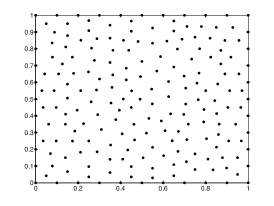
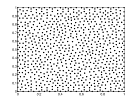
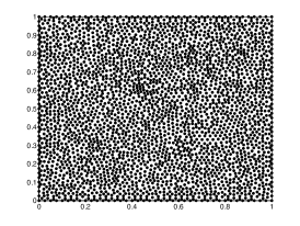
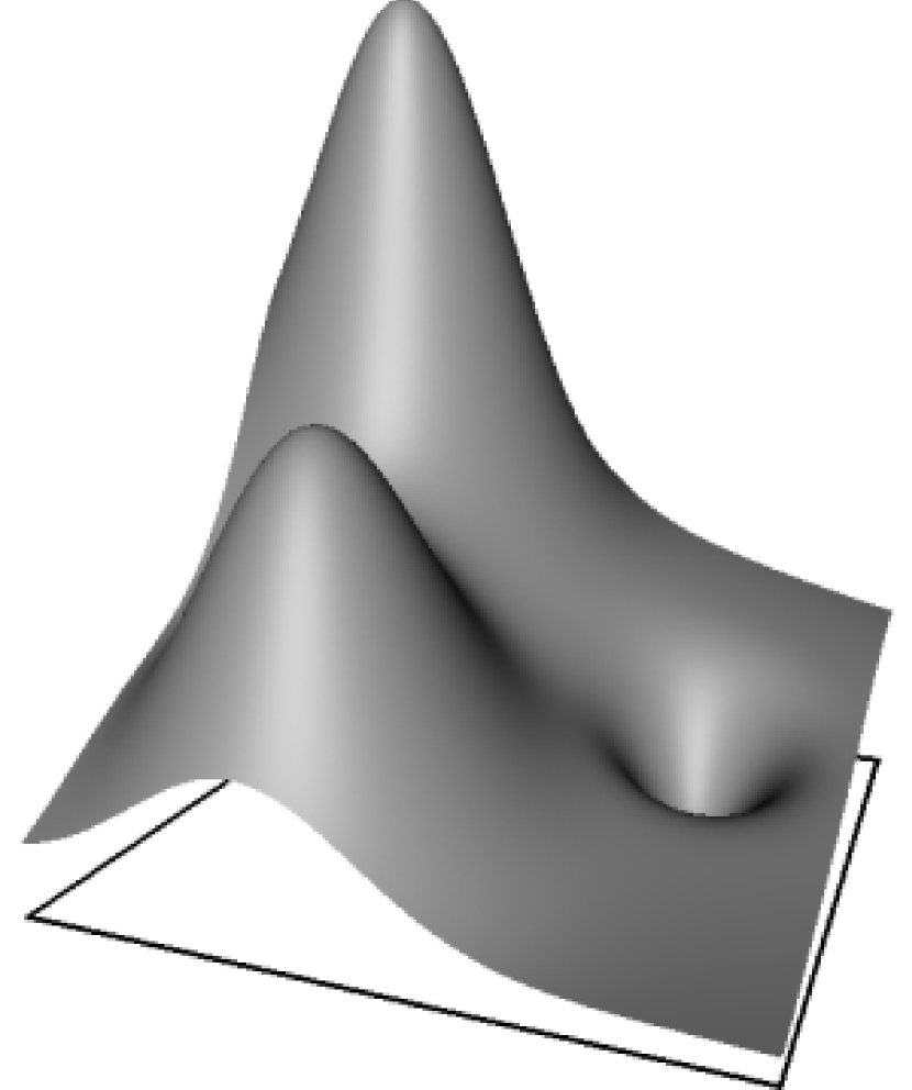
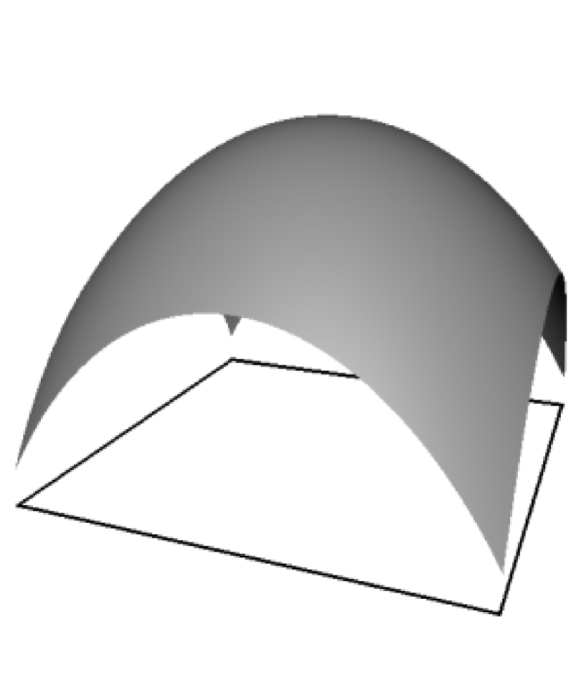
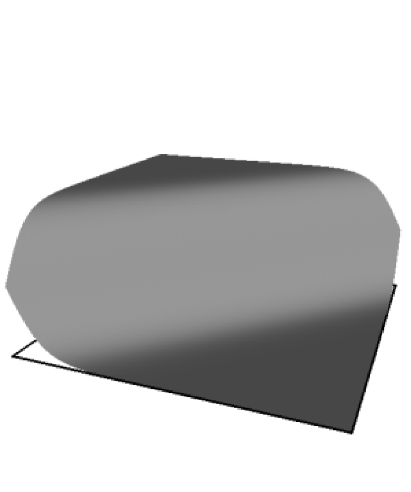
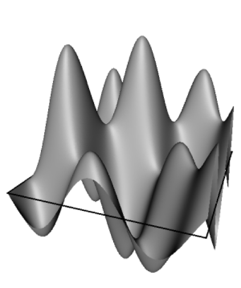
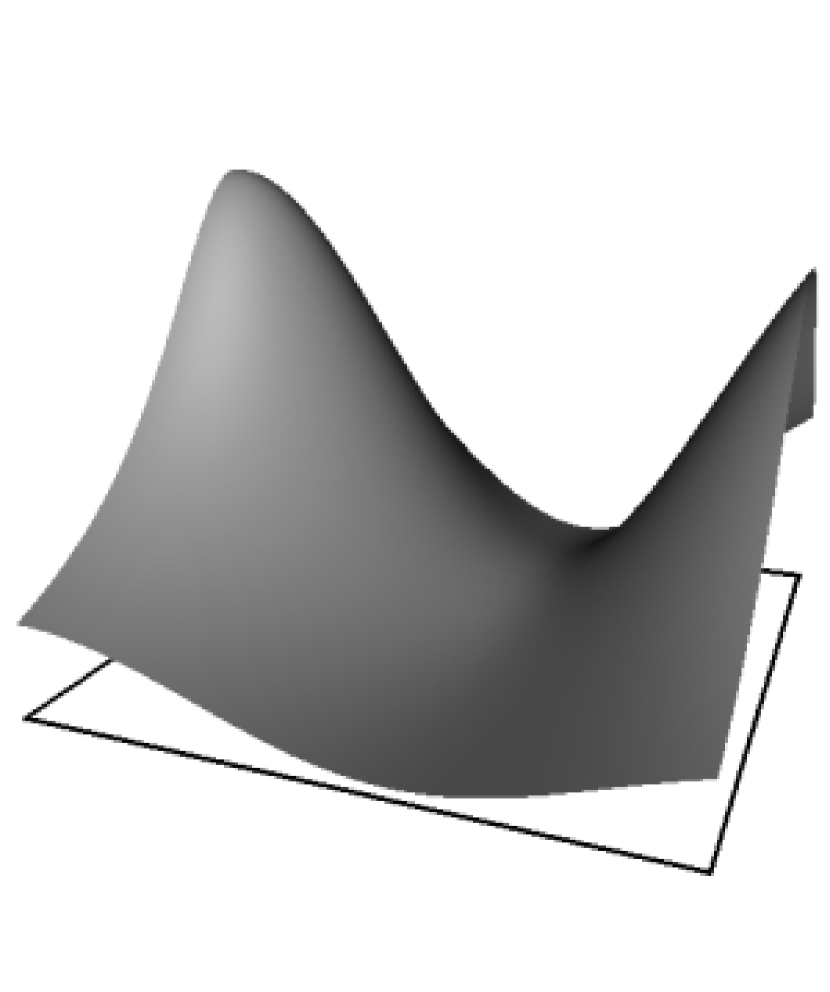
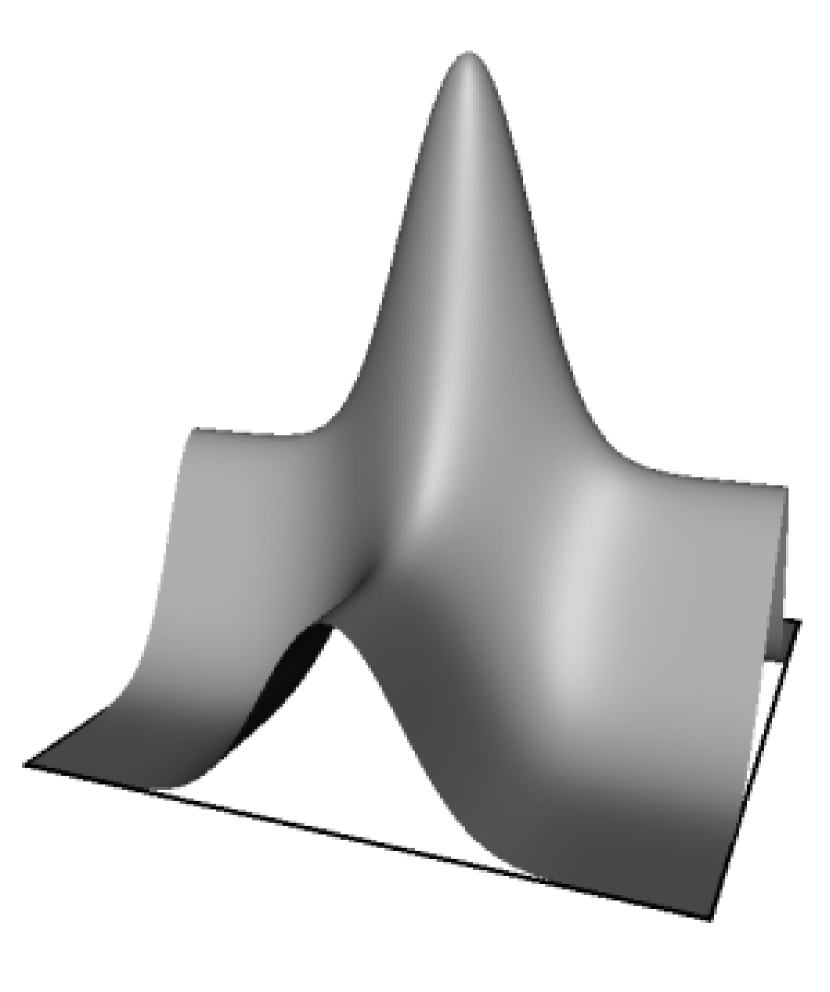
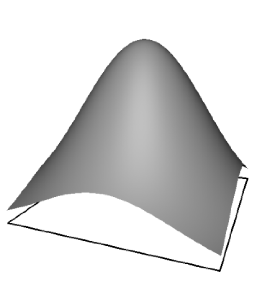
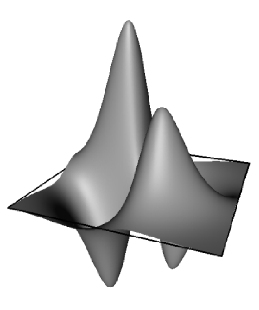
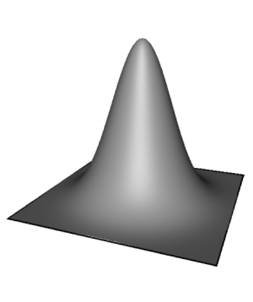
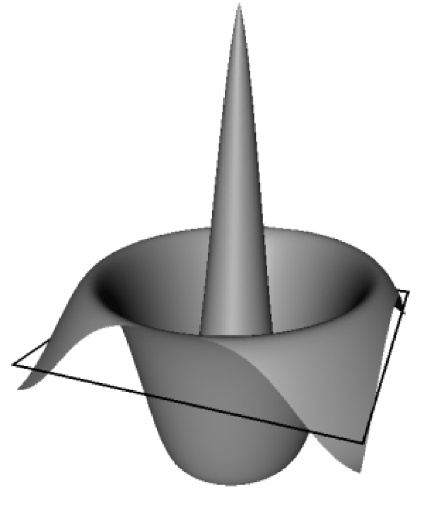
To test the accuracy of approximation of the bivariate Shepard-Bernoulli operator we apply it to different sets of nodes in the rectangle $R=\left[0,1\right]\times\left[0,1\right]$ (see Figure 2) and $10$ test functions (see Figure 3) generally used in the multivariate interpolation of large sets of scattered data [32, 36]. In the following we report the results of some of these experiments.

$f_{1}$

$f_{6}$

$f_{2}$

$f_{7}$

$f_{3}$

$f_{8}$

$f_{4}$

$f_{9}$

$f_{5}$

$f_{10}$

Figure 3. Test functions used in our numerical experiments. The definitions of the test functions can be found in [34].

4.1. Error of approximation when derivative data are given

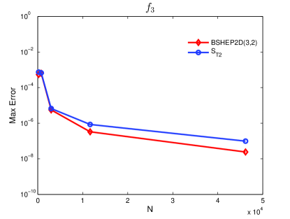
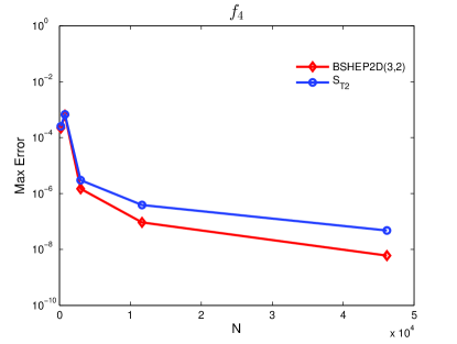
In a first series of experiments, we consider the case in which at each node $V_{i}$ function evaluations and derivative data up to the order $2$ are given. In this case, for each function $f_{i},i=1,\ldots,10$ we compare the numerical results obtained by applying the approximation operator $S_{B_{3}}\left[f\right]$ with those obtained by the local version of the famous Shepard-Taylor operator [21, 40]

(4.1) $$S_{T_{2}}\left[f\right]\left(x,y\right)=\sum\limits_{i=1}^{N}\widetilde{W}_{\mu,i}\left(x,y\right)T_{2}\left[f,V_{i}\right]\left(x,y\right)$$

which uses the same data. We report the results for the first four functions in Figure 4, where we show the maximum interpolation errors, computed for the parameter value $N_{w}=9$. The remaining six functions have a similar behaviour and for this reason we omit them. Numerical results show that the operator $S_{B_{3}}$ improves the accuracy of the operator $S_{T_{2}}$.

Figure 4. Comparison between the maximum approximation error using $S_{T_{2}}$ operator and BSHEP2D(3,2) operators when function evaluations and derivative data up to the order $2$ are given.

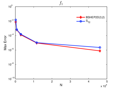
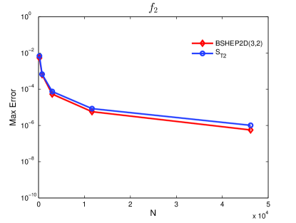
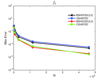
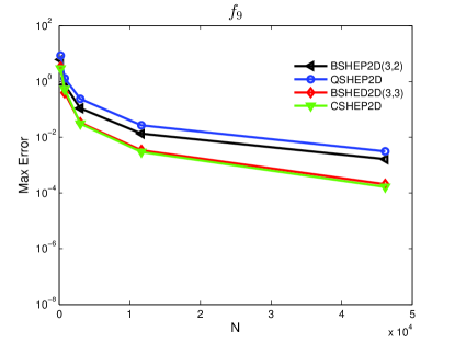
4.2. Error of approximation when only function evaluations are given

In a second series of experiments, we consider the case in which at each node $V_{i}$ only function evaluations are given. In this case, the second order derivatives

(4.2) $$\frac{\partial f}{\partial x},\frac{\partial f}{\partial y},\frac{1}{2}\frac{\partial^{2}f}{\partial x^{2}},\frac{\partial^{2}f}{\partial x\partial y},\frac{1}{2}\frac{\partial^{2}f}{\partial y^{2}}$$

are usually replaced by the coefficients $a_{10},a_{01},a_{20},a_{11},a_{02}$ of the quadratic polynomial

$$Q_{i}\left(x,y\right)=f\left(V_{i}\right)+\sum_{\begin{subarray}{c}r+s=1\\ r\geq 0,s\geq 0\end{subarray}}^{2}a_{rs}\left(x-x_{i}\right)^{r}\left(y-y_{i}\right)^{s}$$

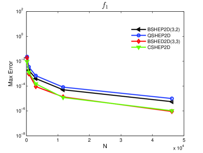
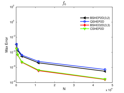
which fits data values $\left(V_{k},f\left(V_{k}\right)\right),k=1,\ldots,N$ on a set of nearby nodes in a weighted least-square sense, as in the definition of operator QSHEP2D [34]. The procedure for computing these coefficients is well detailed in [32] and it is based on the choice of another radius of influence about node $V_{i}$, $R_{q}$, which varies with $i$ and is taken to be just large enough to include $N_{q}$ nodes in $B\left(\boldsymbol{x}_{i},R_{q_{i}}\right)$. At the same time the derivative data (4.2) at $V_{i},i=1,\ldots,N$ can be replaced by the coefficients $b_{10},b_{01},b_{20},b_{11},b_{02}$ of the cubic polynomial

$$C_{i}\left(x,y\right)=f\left(V_{i}\right)+\sum_{\begin{subarray}{c}r+s=1\\ r\geq 0,s\geq 0\end{subarray}}^{3}b_{rs}\left(x-x_{i}\right)^{r}\left(y-y_{i}\right)^{s}$$

which fits the data values $\left(V_{k},f\left(V_{k}\right)\right),k=1,\ldots,N$ on a set of nearby nodes in a weighted least-square sense, as in the definition of operator CSHEP2D in [35]. In the following we denote by BSHEP2D(3,2) the Shepard-Bernoulli operator obtained by substituting the partial derivatives in $S_{B_{3}}\left[f\right]$ with linear combinations of $a_{10},a_{01},a_{20},a_{11},a_{02}$ and by BSHEP2D(3,3) the Shepard-Bernoulli operator obtained by substituting the partial derivatives in $S_{B_{3}}\left[f\right]$ with linear combinations of $b_{10},b_{01},b_{20},b_{11},b_{02}$. Therefore the operator BSHEP2D(3,2) has degree of exactness $2$ as the operator QSHEP2D, while the operator BSHEP2D(3,3) has degree of exactness $3$ as the operator CSHEP2D. We report the results for the first four functions in Figure 5, where we show the maximum interpolation errors, computed for the parameter value $N_{w}=9$ and $N_{q}=13$ for the operator QSHEP2D and $N_{q}=17$ when we replace the derivative data by using the cubic polynomial $C_{i}(x,y)$. The remaining six functions have a similar behaviour and for this reason we omit them. Numerical results show that the operator $S_{B_{3}}$ improves the accuracy of the operator QSHEP2D and is comparable with the operator CSHEP2D.

Figure 5. Comparison between the maximum approximation error using QSHEP2D and CSHEP2D operators and BSHEP2D(3,2) and BSHEP2D(3,3) operator when only function evaluations are given.

With regard to the computational cost we note that the point-triangle associations which reduce the error of the three point interpolation polynomials (2.8) involves an additional cost of $O\left(N\right)$ calculations that do not modify the computational cost of operator QSHEP2D which is $O\left(N\right)$ for uniform distributions of nodes and $O\left(N^{2}\right)$ in worst cases [36]. On the other hand, local basis (1.3) used to define our operators, containing a considerably lower number of nodes compared to the choices recommended by Renka, involve a better localization of the combined operator.

5. Conclusions

In this paper we propose a new definition of the bivariate Shepard-Bernoulli operators which avoids the drawbacks of Catinas extension [8]. These new interpolation operators are realized by using local support basis functions introduced in [23] instead of classical Shepard basis functions and the bivariate three point extension [13] of the generalized Taylor polynomial introduced by F. Costabile in [11]. Their definition requires the association, to each sample point, of a triangle with a vertex in it and other two vertices in its neighborhood. The proposed point-triangle association is carried out to reduce the error of the three point interpolation polynomial. As a consequence, the resulting operator not only inherits interpolation conditions that each three point local interpolation polynomial satisfies at the referring vertex and increases by $1$ the degree of exactness of the Shepard-Taylor operator [21] which uses the same data, but also improves its accuracy. In this sense, the Shepard-Bernoulli operators belong to a recently introduced class of operators for enhancing the approximation order of Shepard operators by using supplementary derivative data [7, 15, 16]. For the general problem of the enhancement of the algebraic precision of linear operators of approximation see the papers [26, 25, 30] and the references therein. Moreover, when applied to the scattered data interpolation problem, the Shepard-Bernoulli operator $S_{B_{3}}$ improves the accuracy of the operator QSHEP2D and is comparable with the operator CSHEP2D by Renka [34, 35]. Finally, the quadratic triangular finite element $P_{2}^{\left[\Delta_{2}\left(V_{1},V_{2},V_{3}\right);V_{3}\right]}[f]\left(\boldsymbol{x}\right)$ can be used to improve the accuracy of approximation of the triangular Shepard method [31].

References

- [1] Atkinson, K.E.: An Introduction to Numerical Analysis. John Wiley & Sons, New York (1978)
- [2] Apostol, T.: Calculus, Vol. 1. John Wiley & Sons, Inc., New York (1967)
- [3] Barnhill,R.E.: Representation and approximation of surfaces. In: Mathematical software III, J.R. Rice, eds. Academic Press, New York, 68-119 (1977)
- [4] Bojanov, Borislav D., Hakopian, H., Sahakian,B.: Spline Functions and Multivariate Interpolations. Kluwer Academic Publishers, Dordrecht (1993)
- [5] Brenner, S.C., Scott, L.R.:The Mathematical Theory of Finite Elements Methods. Springer-Verlag, New York (1994)
- [6] Caira, R., Dell’Accio, F.: Shepard-Bernoulli operators. Mathematics of Computation, 76, 299-321 (2007)
- [7] Caira, R., Dell’Accio, F., Di Tommaso, F.: On the bivariate Shepard-Lidstone operators. Journal of Computational and Applied Mathematics, 236, 1691-1707 (2012)
- [8] Catinas, T.: The bivariate Shepard operator of Bernoulli type. Calcolo 44, 189-202 (2007)
- [9] Chui, C.K., Lai, M.J.: Multivariate vertex splines and finite elements. Journal of Approximation Theory 60, 245-343 (1990)
- [10] Coman, Gh., Trîmbiţaş, R.T.: Combined Shepard univariate operators. East Journal of Approximation 7, 471-483 (2001)
- [11] Costabile,F.A.: Expansions of real functions in Bernoulli polynomials and applications. Conferenze del Seminario di Matematica, Università di Bari 273, 1-13 (1999)
- [12] Costabile,F.A., Dell’Accio,F.: Expansion over a rectangle of real functions in Bernoulli polynomials and applications. BIT 41, 451-464 (2001)
- [13] Costabile,F.A., Dell’Accio,F.: Expansions over a simplex of real functions by means of Bernoulli polynomials. Numerical Algorithms 28, 63-86 (2001)
- [14] Costabile,F.A., Dell’Accio,F.: Lidstone Approximation on the triangle. Applied Numerical Mathematics, 339-361 (2005)
- [15] Costabile,F.A., Dell’Accio,F., Di Tommaso F.: Enhancing the approximation order of local Shepard operators by Hermite polynomials. Computers & Mathematics with Applications, 64, 3641-3655 (2012)
- [16] Costabile,F.A., Dell’Accio,F., Di Tommaso F.: Complementary Lidstone interpolation on scattered data sets. Numerical Algorithms,64, 157-180 (2013)
- [17] Costabile,F.A., Dell’Accio,F., Gualtieri, M.I.: A new approach to Bernoulli polynomials on the Triangle. Rendiconti di Matematica e delle sue Applicazioni, 26, 1-12 (2006)
- [18] Costabile, F.A., Dell’Accio, F., Guzzardi, L.: New bivariate polynomial expansion with only boundary data on the simplex. Calcolo, 45, 177-192 (2008)
- [19] Costabile, F.A., Dell’Accio, F., Luceri, R.: Explicit polynomial expansions of regular real functions by means of even order Bernoulli polynomials and boundary values. Journal of Computational and Applied Mathematics, 176, 77-90 (2005)
- [20] Davis, P.J. Interpolation & Approximation. Dover Publications, Inc., New York (1975)
- [21] Farwig, R.: Rate of convergence of Shepard’s global interpolation formula. Mathematics of Computation, 46, 577-590 (1986)
- [22] Franke, R.: Scattered data interpolation: tests of some methods. Mathematics of Computation 38, 181-200 (1982)
- [23] Franke, R., Nielson, G.: Smooth interpolation of large sets of scattered data. International Journal for Numerical Methods in Engineering, 15, 1691-1704 (1980)
- [24] Gordon, W.J., Wixom, J.A.: Shepard’s Method of ”Metric Interpolation” to Bivariate and Multivariate Interpolation. Mathematics of Computation, 32, 253-264 (1978)
- [25] Guessab, A., Nouisser, O., Schmeisser, G.: Multivariate approximation by a combination of modified Taylor polynomials. Journal of Computational and Applied Mathematics, 196, 162-179 (2006)
- [26] Xuli, H.: Multi-node higher order expasions of a functions. Journal of Approximation Theory 124, 242-253 (2003)
- [27] Hoschek, J., Lasser, D.: Fundamentals of Computer Aided Geometric Design. A. K. Peters, USA (1989)
- [28] Jordan, R.: Calculus of Finite Differences. Chelsea Publishing Co., New York (1960)
- [29] Kraaijpoel, D., van Leeuwen, L.: Raising the order of multivariate approximation schemes using supplementary derivative data. Procedia Computer Science, 1, 307-316 (2010)
- [30] Lamnii, M., Mazroui, A., Tijini, A.: Raising the approximation order of multivariate quasi-interpolants. BIT Numerical Mathematics, DOI 10.1007/s10543-014-0470-8 (2014)
- [31] Little, F.: Convex Combination Surfaces. In Surfaces in Computer Aided Geometric Design, 99-108 (1982)
- [32] Renka, R.J., Cline, A.K.: A triangle-based interpolation method. Rocky Mountain Journal of Mathematics, 14, 223-237 (1984)
- [33] Renka, R.J.: Multivariate Interpolation of Large Sets of Scattered Data. ACM Transactions on Mathematical Software, 14, 139-148 (1988)
- [34] Renka, R.J.: Algorithm 660, QSHEP2D: Quadratic Shepard Method for Bivariate Interpolation of Scattered Data. ACM Transactions on Mathematical Software, 14, 149-150 (1988)
- [35] Renka, R.J.: Algorithm 790, CSHEP2D: Cubic Shepard Method for Bivariate Interpolation of Scattered Data. ACM Transactions on Mathematical Software, 25, 70-73 (1999)
- [36] Renka, R.J., Brown, R.: Algorithm 792: Accuracy Tests of ACM Algorithms for Interpolation of Scattered Data in the Plane. ACM Transactions on Mathematical Software, 25, 78-94 (1999)
- [37] Shepard, D.: A two-dimensional interpolation function for irregularly-spaced data. In Proceedings of the 1968 23rd ACM National Conference, ACM Press, New York, 517-524 (1968)
- [38] Wendland, H.: Scattered Data Approximation. Cambridge University Press (2005)
- [39] Whitney, H.: Functions differentiable on the boundaries of regions. Annals of Mathematics 35, 482-485 (1934)
- [40] Zuppa, C.: Error estimates for modified local Shepard’s interpolation formula. Applied Numerical Mathematics, 49, 245-259 (2004)