Quantum Wronskian approach to six-point gluon scattering amplitudes at strong coupling

Abstract

We study the six-point gluon scattering amplitudes in ${\cal N}=4$ super Yang-Mills theory at strong coupling based on the twisted ${\mathbb{Z}}_{4}$-symmetric integrable model. The lattice regularization allows us to derive the associated thermodynamic Bethe ansatz (TBA) equations as well as the functional relations among the Q-/T-/Y-functions. The quantum Wronskian relation for the Q-/T-functions plays an important role in determining a series of the expansion coefficients of the T-/Y-functions around the UV limit, including the dependence on the twist parameter. Studying the CFT limit of the TBA equations, we derive the leading analytic expansion of the remainder function for the general kinematics around the limit where the dual Wilson loops become regular-polygonal. We also compare the rescaled remainder functions at strong coupling with those at two, three and four loops, and find that they are close to each other along the trajectories parameterized by the scale parameter of the integrable model.

June 2014

1. Introduction

The gluon scattering amplitudes in ${\cal N}=4$ super Yang-Mills theory are a subject of great interest in recent years. In the planar limit, they are dual to the null-polygonal Wilson loops whose segments are light-like and proportional to external gluon momenta [1, 2, 3, 4, 5]. The duality implies a conformal symmetry in the dual space [1, 6, 7, 8]. This dual conformal symmetry strongly constrains the form of the amplitudes. In particular, the maximal helicity violating (MHV) amplitude is expressed as a sum of the Bern, Dixon and Smirnov (BDS) formula [9] and a finite remainder (remainder function), which is a function of the cross-ratios of the cusp coordinates for the null polygon.

The amplitudes have been studied intensively from both weak- and strong-coupling sides. At weak coupling, recent developments using the mixed motive theory have made it possible to evaluate the remainder function for the six-point amplitudes up to four-loop level [10]. Moreover a method based on the OPE and integrability has been proposed to calculate the scattering amplitudes in this theory, which is expected to be applicable to the intermediate coupling region[11, 12, 13, 14].

At strong coupling, the AdS/CFT correspondence asserts explicit relations between ${\cal N}=4$ super Yang-Mills theory and the superstring theory in AdS${}_{5}\times$S⁵. Alday and Maldacena have thereby proposed that the MHV amplitude can be evaluated by the area of the minimal surfaces in AdS with a null-polygonal boundary along the Wilson loop [1]. It turns out later that the remainder function for the null-polygonal minimal surfaces is calculated with the help of integrability [15]. Namely it is obtained by solving the Y-system or the thermodynamic Bethe ansatz (TBA) system related to certain two-dimensional quantum integrable systems [16, 17, 18]. The cross-ratios are given by the Y-functions at special values of the spectral parameter and the remainder function is expressed by the free energy of the TBA system and the Y-functions.

For the null-polygonal minimal surfaces in AdS₃ and AdS₄ space-time, the relevant integrable systems are the homogeneous sine-Gordon models [19] with purely imaginary resonance parameters [18], which are the perturbed SU($N$)_k/U(1)^N-1 coset conformal field theory (CFT) at level $k=2$ and $4$, respectively. Around the limit where the null boundary becomes regular polygonal, corresponding to the UV limit of the two-dimensional systems, the remainder functions are calculated analytically for lower point amplitudes [20, 21, 22]. There, the free-energy part is evaluated by the standard bulk conformal perturbation theory (CPT). In order to evaluate the Y-functions, the $g$-function or the boundary entropy is utilized because the Y-function itself is not well incorporated in quantum field theory. The boundary CPT then efficiently yields the analytic expansions of the Y-functions. The resultant remainder functions are observed to be close to the two-loop results after an appropriate normalization/rescaling. Numerically, one also finds that this similarity extends beyond the UV limit. The minimal surfaces in these cases, however, give the amplitudes with some specific kinematic configurations of gluon momenta.

The null-polygonal minimal surface in AdS₅ with six cusps is the simplest non-trivial example that allows the most general kinematic configuration. At strong coupling, the relevant two-dimensional system is the $\mathbb{Z}_{4}$-symmetric integrable model [23, 24, 25] with a boundary twist [26]. The remainder function around the UV limit in this case has been studied in detail in [27]. Although the free-energy part is analytically evaluated by the bulk CPT for the twisted $\mathbb{Z}_{4}$-parafermion, the expansion of the Y-functions there is determined by numerical fitting. The difference from the the AdS₃ and AdS₄ cases come from the fact that the TBA equations in the AdS₅ case have a twist parameter, and it is unclear how to construct the $g$-function with this twist parameter.

Given the analytic results at weak coupling as well as the OPE method for finite coupling, the analytic data at strong coupling would provide pieces of the whole picture of the scattering amplitudes. They would also be useful for a check of the finite-coupling analysis. In this report, we thus decide to devote ourselves to the analytic expansions of the remainder function for the general kinematics.

In order to overcome the problem mentioned above, we take below another route for the UV expansion of the Y-functions, which does not rely on the $g$-function. Instead, our analysis is based on a seminal work by Bazhanov, Lukyanov and Zamolodchikov [28, 29], where the role of quantum monodromy matrix is clarified in the minimal CFT, ${\cal M}_{2,2n+3}$, perturbed by the $\Phi_{1,3}$ operator. Most remarkably, a new object in field theories, Baxter’s Q operator, is introduced in this work. They noted the importance of the fundamental relations among the T- and Q-functions, the quantum Wronskian relation [29]. The T- and Y-systems can be regarded as colloraries of this. The Q operators and the quantum Wronskian relation have also played important roles in the non-equilibrium current problem [30], in the ODE/IM correspondence [31], in the spectral problem of the AdS₅/CFT₄ correspondence [32] and so on.

In this report, we provide a yet another application: the quantum Wronskian relation is very efficient in obtaining the analytic expansion of the Y-functions particularly in the CFT limit. Specifically, we apply it, for the first time, to the $\mathbb{Z}_{4}$-symmetric integrable model or its lattice regularization. The lattice regularization adopted here allows one to elucidate the analyticity of the T-/Y-functions numerically. The expansion of the Y-functions around the UV limit is then determined analytically up to and including the terms of order (mass)${}^{\frac{4}{3}}$. A series of the higher-order coefficients is also determined recursively.

Combined with the free-energy part, the UV expansion of the Y-functions gives the analytic expansion of the six-point reminder function for the general kinematic configuration. We also compare the strong-coupling results with the perturbative ones, and find that the rescaled remainder functions are close to each other for large ranges of the parameters. This is in accord with the previous observations in the AdS₃ and AdS₄ cases [33, 20, 21, 22] as well as in the perturbative cases [34, 10].

This paper is organized as follows: In Section 2, we review the TBA-system for the six-point gluon scattering amplitudes at strong coupling and express the remainder functions using Y-functions. In Section 3, we reconsider the Y-/T-functions based on the lattice model. Taking the scaling limit, we derive the TBA system for the amplitudes. In Section 4, we study the CFT limit of the TBA system. Based on the T-Q relation and the quantum Wronskian relation, we calculate the analytic expansion of the Y-function in the CFT limit. The detailed analysis of the asymptotics of the related spectral determinant based on non-linear integral equations is studied in Appendix A. In Section 5, we apply the analytic expansion of the Y-functions to determine the leading expansion of the remainder function for the six-point amplitudes and compare it with the perturbative calculations.

2. Y-system and TBA for scattering amplitudes at strong coupling

Let us begin with a review on the evaluation of the six-point MHV amplitudes at strong coupling using TBA of the twisted ${\mathbb{Z}}_{4}$-symmetric integrable model.

2.1. Hitchin system and Stokes data

Alday and Maldacena proposed a method of computing the gluon scattering amplitudes in ${\cal N}=4$ super Yang–Mills using the AdS/CFT correspondence [1, 15]. Consider the the scalar part of the $n$-point gluon MHV scattering amplitudes in the strong coupling limit, and factor out the contribution of the tree amplitudes. According to [1], the result can be evaluated by computing the area $A$ of the corresponding classical open string solutions in AdS₅ spacetime:

$$\frac{{\text{(amplitude)}}}{\text{(tree)}}\sim{\rm e}^{-\frac{\sqrt{\lambda}}{2\pi}A}$$

where $\lambda$ denotes the ’t Hooft coupling. A string solution represents a minimal surface whose boundary is a polygon located on the boundary of AdS₅. The polygon consists of $n$ null edges given by the $n$ momenta of incoming gluons. Note that the amplitudes are defined in space-time with signature (3,1), (2,2) or (1,3).

The equations of motion of the string under the Virasoro constraints are rephrased as the SU(4) Hitchin equations for the connections $(A_{z},A_{\bar{z}})$ and the adjoint scalar fields $(\Phi_{z},\Phi_{\bar{z}})$ with the ${\mathbb{Z}}_{4}$ automorphism[16]. They are equivalently presented by the linear equations for a four component vector $q(z,{\bar{z}};\zeta)$,

$$\Bigl{(}D_{z}+\zeta^{-1}\Phi_{z}\Bigr{)}q(z,{\bar{z}};\zeta)=0,\qquad\Bigl{(}D_{\bar{z}}+\zeta\Phi_{\bar{z}}\Bigr{)}q(z,{\bar{z}};\zeta)=0,$$ (2.1)

with appropriate boundary conditions. Here $D_{z}$ and $D_{\bar{z}}$ denote the covariant derivatives and $\zeta$ stands for the spectral parameter. The explicit forms of $D_{z}$ and $D_{\bar{z}}$ are given in [16]. The information of the null polygon is encoded in the asymptotic behavior of $\Phi_{z}$, which is diagonalized at infinity by an appropriate gauge transformation:

$$h^{-1}\Phi_{z}h \to \frac{1}{\sqrt{2}}{\text{diag}}\bigl{(}P(z)^{1/4},-iP(z)^{1/4},-P(z)^{1/4},iP(z)^{1/4}\bigr{)}.$$ (2.2)

The polynomial degree of $P(z)$ is $n-4$ and its coefficients parameterize the shape of the polygon. When $n>4$, the linear equation necessarily possesses irregular singularity at infinity, which implies the Stokes phenomena. Customarily, the whole complex plane is divided into sectors,

$$W_{k}:\frac{\pi(2k-3)}{n}+\frac{4}{n}\arg\zeta<\arg z<\frac{\pi(2k-1)}{n}+\frac{4}{n}\arg\zeta.$$ (2.3)

We denote by $s_{k}(z,{\bar{z}};\zeta)$, the most recessive solution as $|z|\to\infty$ in $W_{k}$. One can consistently choose $(s_{k},s_{k+1},s_{k+2},s_{k+3})$ as a linearly independent basis in $W_{k}$. This implies a linear dependent relation among five neighboring $s_{j}$’s,

$$s_{k}+s_{k+4}=a_{k}s_{k+1}+b_{k+1}s_{k+2}+c_{k+3}s_{k+3},$$ (2.4)

where $b_{k+1}$ and $c_{k+1}$ are some constants. Note the periodicity $b_{i+3}=b_{i}$.

The normalization of $s_{j}(z,{\bar{z}};\zeta)$ is fixed such that

$$\langle s_{j},s_{j+1},s_{j+2},s_{j+3}\rangle=1,$$ (2.5)

where $\langle s_{i},s_{j},s_{k},s_{l}\rangle\equiv\det(s_{i}s_{j}s_{k}s_{l})$. The ${\mathbb{Z}}_{4}$ automorphism results in the following relations for the Stokes data,

$$\langle s_{k},s_{k+1},s_{j},s_{j+1}\rangle(\zeta) = \langle s_{k-1},s_{k},s_{j-1},s_{j}\rangle(i\zeta),$$ (2.6)

$$\langle s_{j},s_{k},s_{k+1},s_{k+2}\rangle(\zeta) = \langle s_{j},s_{j-1},s_{j-2},s_{k}\rangle(i\zeta).$$ (2.7)

Below, we confine our argument to the $n=6$ case where

$$P(z)=z^{2}-U.$$ (2.8)

For $W_{j+6}=W_{j}$, we shall impose the boundary condition,

$$s_{j+6}=\mu^{(-1)^{j}}s_{j}.$$ (2.9)

The multiplier $\mu$ is parametrized as

$$\mu=e^{i\frac{3}{2}\phi},$$ (2.10)

where $\phi$ is real for solutions in the $(1,3)$ or in the $(3,1)$ signature of the four-dimensional space-time whereas it is purely imaginary for the $(2,2)$ signature. It also appears, e.g., in the relation among $b_{i}$,

$$b_{1}b_{2}b_{3}=b_{1}+b_{2}+b_{3}+\mu+\mu^{-1}.$$ (2.11)

2.2. Y-functions, TBA and evaluation of area

The key ingredients in the following discussion are the Y-functions, which are defined explicitly by

$$Y_{1}(\theta) = -\langle s_{2},s_{3},s_{5},s_{6}\rangle(e^{\theta}),$$ (2.12)

$$Y_{2}(\theta) = \langle s_{1},s_{2},s_{3},s_{5}\rangle\langle s_{2},s_{4},s_{5},s_{6}\rangle(e^{\theta+\pi i/4}),$$ (2.13)

$$Y_{3}(\theta) = Y_{1}(\theta).$$ (2.14)

Then it was shown in [16] that the Hirota bilinear identities (or Plücker relations), as well as the relations (2.9), (2.6) and (2.7), lead to the following Y-system,

$$Y_{1}\left(\theta+\frac{\pi i}{4}\right)Y_{1}\left(\theta-\frac{\pi i}{4}\right) = 1+Y_{2}(\theta),$$ (2.15)

$$Y_{2}\left(\theta+\frac{\pi i}{4}\right)Y_{2}\left(\theta-\frac{\pi i}{4}\right) = \bigl{(}1+\mu Y_{1}(\theta)\bigr{)}\bigl{(}1+\mu^{-1}Y_{1}(\theta)\bigr{)}.$$ (2.16)

The asymptotic behavior of the Y-functions is shown to be

$$\log Y_{1}(\theta)\to|Z|e^{\pm(\theta-i\varphi)},\qquad\log Y_{2}(\theta)\to\sqrt{2}|Z|e^{\pm(\theta-i\varphi)}$$

$$\mbox{for}\quad{\rm Re\,}\theta\to\pm\infty,\qquad\varphi-\frac{\pi}{4}<{\rm Im\,}\theta<\varphi+\frac{\pi}{4},$$ (2.17)

where $Z$ is a complex parameter with phase $\varphi$. This is related to the moduli parameter $U$ in (2.8) as

$$Z\equiv|Z|e^{i\varphi}=U^{\frac{3}{4}}\int_{-1}^{1}(1-t^{2})^{\frac{1}{4}}dt=\frac{\sqrt{\pi}\Gamma(\frac{1}{4})}{3\Gamma(\frac{3}{4})}U^{\frac{3}{4}}.$$ (2.18)

We further introduce

$$\epsilon(\theta)=\log Y_{1}(\theta+i\varphi),\qquad{\tilde{\epsilon}}(\theta)=\log Y_{2}(\theta+i\varphi).$$ (2.19)

The asymptotic behavior (2.2.), together with the assumption of the analyticity of $\epsilon,{\tilde{\epsilon}}$ in the strip $\,{\rm Im}\,\theta\in(-\frac{\pi}{4},\frac{\pi}{4})$, leads to the integral equations,

$$\epsilon = 2|Z|\cosh\theta+{\cal K}_{2}\ast\log\bigl{(}1+e^{-{\tilde{\epsilon}}}\bigr{)}+{\cal K}_{1}\ast\log\bigl{(}1+\mu e^{-\epsilon}\bigr{)}\bigl{(}1+\mu^{-1}e^{-\epsilon}\bigr{)},$$ (2.20)

$${\tilde{\epsilon}} = 2\sqrt{2}|Z|\cosh\theta+2{\cal K}_{1}\ast\log\bigl{(}1+e^{-{\tilde{\epsilon}}}\bigr{)}+{\cal K}_{2}\ast\log\bigl{(}1+\mu e^{-\epsilon}\bigr{)}\bigl{(}1+\mu^{-1}e^{-\epsilon}\bigr{)},\qquad$$ (2.21)

where

$${\cal K}_{1}(\theta)=\frac{1}{2\pi\cosh\theta},\qquad{\cal K}_{2}(\theta)=\frac{\sqrt{2}\cosh\theta}{\pi\cosh 2\theta},\qquad$$ (2.22)

and the symbol $*$ denotes the convolution, $f\ast g=\int_{-\infty}^{\infty}d\theta^{\prime}f(\theta-\theta^{\prime})g(\theta^{\prime})$. These turn out be identical to the TBA equations for the $\mathbb{Z}_{4}$-symmetric integrable model [23, 24, 25] twisted by $\mu$. The equations (2.20) and (2.21) determine $\epsilon$ and ${\tilde{\epsilon}}$ in the strip completely.

In the original setting, the geometric data such as cross-ratios are given first, and then the area of the surfaces should be evaluated. Below, we slightly deform this logic: the TBA equations are given first, then the cross-ratios and the area are evaluated second. Once the TBA equations are solved, the coefficient $b_{k}$ in eq. (2.4) and the cross-ratios of gluon momenta are given by

$$b_{k}=Y_{1}\left(\frac{(k-1)\pi i}{2}\right),\qquad U_{k}=1+Y_{2}\left(\frac{(2k+1)\pi i}{4}\right),$$ (2.23)

for $k=1,2,3$ (mod 3), where

$$U_{1}=b_{2}b_{3}=\frac{x_{14}^{2}x_{36}^{2}}{x_{13}^{2}x_{46}^{2}},\qquad U_{2}=b_{3}b_{1}=\frac{x_{25}^{2}x_{14}^{2}}{x_{24}^{2}x_{15}^{2}},\qquad U_{3}=b_{1}b_{2}=\frac{x_{36}^{2}x_{25}^{2}}{x_{35}^{2}x_{26}^{2}}.$$ (2.24)

The cusp coordinates $x_{j}$ are related to the external momenta through $p_{j}=x_{j}-x_{j+1}$. In the literature, $u_{k}:=1/U_{k}$ are often used as a basis of independent cross-ratios for the six-point case. The number of the independent cross-ratios matches that of the parameters in the TBA system $(|Z|,\varphi,\mu)$.

Naively, the values of $Y_{j}$ outside the analytic strip are necessary in order to evaluate $U_{k}\,(1\leq k\leq 3)$. Although this can be accomplished by the analytic continuation in principle, we can avoid this by a clever choice of quantities. For example, suppose $\varphi$ is negative and small. Two quantities, $b_{1}$ and $U_{2}=U_{-1}$, are readily calculated by (2.23). Then one evaluates $b_{3}$ by the second equation in (2.24). The final piece, $b_{2}$, is obtained from (2.11). Given $b_{i}$, other cross ratios are now accessible via (2.24). Alternatively, one may also use the Y-system (2.15), (2.16) as recurrence relations to generate $Y_{j}(k\pi i/4)$ for any $k\in{\mathbb{Z}}$ from a set of $Y_{j}(k^{\prime}\pi i/4)$ in the analytic strip. As discussed shortly, the Y-functions have the periodicity $Y_{j}(\theta+3\pi i/2)=Y_{j}(\theta)$, and thus the procedure terminates after a few steps.

We are now in position to write down the area $A$ of the 6-cusp solutions or the scalar magnitude of the gluon scattering amplitudes in the strong coupling limit. Instead of $A$ itself, we deal with the finite remainder defined by

$$R=A_{\mbox{\scriptsize BDS}}-A,$$ (2.25)

where $A_{\mbox{\scriptsize BDS}}$ is the all-order ansatz for the MHV amplitude proposed by Bern, Dixon and Smirnov[9], including the divergent part. The present formulation then yields

$$R = \Delta A_{\rm BDS}-A_{\mbox{\scriptsize periods}}-A_{\mbox{\scriptsize free}},$$ (2.26)

and each part reads

$$\Delta A_{\rm BDS} = -\frac{1}{4}\sum_{k=1}^{3}\operatorname{Li_{2}}\left(1-U_{k}\right),$$ (2.27)

$$A_{\mbox{\scriptsize periods}} = |Z|^{2},$$ (2.28)

$$A_{\mbox{\scriptsize free}} = \frac{1}{2\pi}\int_{-\infty}^{\infty}d\theta\biggl{(}2|Z|\cosh\theta\log\bigl{(}1+\mu e^{-\epsilon(\theta)}\bigr{)}\bigl{(}1+\mu^{-1}e^{-\epsilon(\theta)}\bigr{)}$$ (2.29)

$$\hskip 50.00008pt{}+2\sqrt{2}|Z|\cosh\theta\log\bigl{(}1+e^{-{\tilde{\epsilon}}(\theta)}\bigr{)}\biggr{)}.$$

The minus of the last term $F=-A_{\rm free}$ coincides with the free energy whereas $2|Z|$ is identified with the mass/scale parameter of the ${\mathbb{Z}}_{4}$-symmetric integrable model. The overall coupling dependence $\sqrt{\lambda}$ has been omitted above.

Within the framework described above, the numerical solutions of (2.20) and (2.21) yield explicit evaluation of the gluon scattering amplitudes[27] . Although the analytic solution to the TBA equations for generic $Z$ and $\mu$ is beyond our reach, two limiting cases are accessible [36]. One is the limit where $|Z|\to\infty$. In this case, the integrable model reduces to a free massive theory, and the free-energy part $A_{\rm free}$ and the Y-functions $Y_{j}(\theta)$ are expanded by multiple integrals. Via analytic continuation, this limit is also relevant for the amplitudes in the Regge limit [37, 38]. Another limit is $|Z|\to 0$, which we are interested in here.

When $|Z|$ is strictly zero, $A_{\rm free}$ and $Y_{j}$ are obtained as the central charge of the ${\mathbb{Z}}_{4}$-parafermion theory and a solution to the constant Y-system, respectively. Moreover, for small $|Z|$ the free-energy part is expanded by the bulk conformal perturbation theory (CPT). The Y-functions are expanded by the boundary CPT through the relation to the $g$-function for $\mu=1$ [22], corresponding to the minimal surfaces in AdS₄. For generic $\mu$, however, it is still unclear how to incorporate $\mu$ in the framework of the boundary CPT.

In the following, we take an approach to the problem, which is different from any of the above, and is based on the integrable field theoretical structure proposed in [29]. This allows us to analytically evaluate the Y-functions for small $|Z|$, as shown in section 4..

3. T-functions from the lattice regularization and their scaling limit

In this section we embed the Y-system into another tractable object in integrable systems, the T-system. This enable us to apply the machinery of the latter to evaluate the Y-functions for small $|Z|$ in the next section.

There are several ways to introduce the T-system which is equivalent to the Y-system in (2.15) and (2.16). Here we start with the lattice regularization[39]. One advantage of this choice is that analyticity assumptions, necessary to derive the TBA equations, can be checked numerically.

As is well known, the $\mathbb{Z}_{4}$ parafermion model is related to the spin-${1\over 2}$ XXZ model. Its Hamiltonian and spectrum can be studied from the transfer matrix. In order to define the latter, we introduce $R(v)$, the $U_{q}(\widehat{\mathfrak{sl}_{2}})$ $R$ matrix of spin $\frac{1}{2}$ representation:

$$R(v) =\begin{pmatrix}a(v)&&&&\\ &b(v)&c(v)&&\\ &c^{-1}(v)&b(v)&&\\ &&&a(v)&\end{pmatrix},$$

$$a(v) =\frac{\sin(v+\gamma)}{\sin\gamma},\qquad b(v)=\frac{\sin(v)}{\sin\gamma},\qquad c(v)={\rm e}^{-v},$$

where $q={\rm e}^{i\gamma}$. Let $V^{(m)}$ be the $m+1$ dimensional $U_{q}(\mathfrak{sl}_{2})$ module and $V^{(m)}(v)$ be the corresponding $U_{q}(\widehat{\mathfrak{sl}_{2}})$ module. By $V^{(m)}_{i}(v)$ we mean its i-th copy. The $R$ matrix acting on $V_{i}^{(1)}(v_{i})\otimes V^{(1)}_{j}(v_{j})$ is denoted by $R_{i,j}(v_{i}-v_{j})$.

Then one can construct an inhomogeneous transfer matrix ${\mathbf{T}}_{1}(x)$ acting on $2N$ sites by,

$${\mathbf{T}}_{1}(x)={\rm Tr}_{0}D_{\phi}R_{0,2N}(ix+i\Lambda)R_{0,2N-1}(ix-i\Lambda)\cdots R_{0,2}(ix+i\Lambda)R_{0,1}(ix-i\Lambda),$$ (3.1)

where suffix 0 denotes the auxiliary space. The spectral parameter $x$ is set via $v=ix$ for later convenience. We have also introduced the diagonal twist matrix $D_{\phi}=[{\rm e}^{-\frac{\phi}{2}i},{\rm e}^{\frac{\phi}{2}i}]$ under the trace. The quantity $\mu={\rm e}^{i\frac{3}{2}\phi}$ is to be identified with the multiplier in (2.10).

To diagonalize ${\mathbf{T}}_{1}$, Baxter[40] ingeniously introduced an operator ${\mathbf{Q}}$ which commutes with ${\mathbf{T}}_{1}(x)$. They satisfy Baxter’s TQ relation,

$${\mathbf{T}}_{1}(x){\mathbf{Q}}(x)=\Phi(x+i\frac{\gamma}{2}){\mathbf{Q}}(x-i\gamma)+\Phi(x-i\frac{\gamma}{2}){\mathbf{Q}}(x+i\gamma),$$ (3.2)

where

$$\Phi(x)=\bigl{(}-4\sinh(x-\Lambda)\sinh(x+\Lambda)\bigr{)}^{N}.$$

Below we shall consider ${\mathbf{T}}_{1}$ and ${\mathbf{Q}}$ on their common eigenspace, thus we do not distinguish operators from their eigenvalues. The eigenvalue of ${\mathbf{Q}}$ is explicitly written with a set of Bethe roots $\{x_{j}(\phi)\}$ with twist $\phi$,

$$\qquad{\mathbf{Q}}(x)={\rm e}^{\frac{x}{2\gamma}\phi}\prod_{j=1}^{m}2\sinh(x-x_{j}(\phi)).$$

This, together with (3.2), parameterizes the eigenvalue of the transfer matrix.

The fusion method generates a series of vertex models such that the auxiliary space is $V^{(j)}(v)$. Let ${\mathbf{T}}_{j}(x)$ be the corresponding inhomogeneous transfer matrix, with a suitable normalization. By construction $\{{\mathbf{T}}_{j}(x)\}$ constitute a commutative family and they satisfy the T-system of SU(2) type,

$${\mathbf{T}}_{j}(x+\frac{\gamma}{2}i){\mathbf{T}}_{j}(x-\frac{\gamma}{2}i)=f_{j}(x)+{\mathbf{T}}_{j+1}(x){\mathbf{T}}_{j-1}(x),\qquad j\in\mathbb{N}$$ (3.3)

where

$${\mathbf{T}}_{0}(x) :=\Phi(x),\qquad f_{j}(x)={\mathbf{T}}_{0}(x+\frac{j+1}{2}\gamma i){\mathbf{T}}_{0}(x-\frac{j+1}{2}\gamma i).$$

Note the periodicity of ${\mathbf{T}}_{j}(x)$ in the present normalization is

$${\mathbf{T}}_{j}(x+\pi i)={\mathbf{T}}_{j}(x).$$ (3.4)

There is an additional relation when $q$ is at a root of unity, which is crucial in obtaining a closed set of functional relations. From now on we fix

$$\gamma=\frac{2\pi}{3}.$$ (3.5)

Then the desired relation is

$${\mathbf{T}}_{3}(x)={\mathbf{T}}_{1}(x)+{\mathbf{T}}_{0}(x)\bigl{(}\mu+\mu^{-1}).$$ (3.6)

The equation for $j=2$ in (3.3) can be thus rewritten as

$${\mathbf{T}}_{2}(x+\frac{\pi}{3}i){\mathbf{T}}_{2}(x-\frac{\pi}{3}i)=({\mathbf{T}}_{1}(x)+\mu{\mathbf{T}}_{0}(x))({\mathbf{T}}_{1}(x)+\mu^{-1}{\mathbf{T}}_{0}(x)),$$ (3.7)

thereby yielding a closed functional relations among ${\mathbf{T}}_{1}$ and ${\mathbf{T}}_{2}$.

Below we will show that (3.3) for $j=1$ and (3.7) can be transformed into TBA equations. Before doing this, we elucidate the analytic properties of ${\mathbf{T}}_{j}$ deduced from numerics, as a merit in the lattice regularization. By definition, ${\mathbf{T}}_{j}$ has $2N$ zeros and has no poles in complex $x$ plane. Led by numerical observations we conjecture that all zeros of ${\mathbf{T}}_{1}(x)$ are on the $\,{\rm Im}\,x=\frac{\pi}{2}$ line while those of ${\mathbf{T}}_{2}(x)$ are on the real axis in the ground state. Below, quantities which have no zeros and poles in the strip including the real axis will play an important role. We thus define

$${\mathbf{T}}^{\vee}_{j}(x)={\mathbf{T}}_{j}(x+\frac{(j-1)\pi}{2}i)\qquad j=1,2.$$ (3.8)

Then the closed functional relations now read

$${\mathbf{T}}^{\vee}_{1}(x+\frac{\pi}{6}i){\mathbf{T}}^{\vee}_{1}(x-\frac{\pi}{6}i) =f_{1}(x+\frac{\pi}{2}i)+{\mathbf{T}}_{0}(x+\frac{\pi}{2}i){\mathbf{T}}^{\vee}_{2}(x),$$

$${\mathbf{T}}^{\vee}_{2}(x+\frac{\pi}{6}i){\mathbf{T}}^{\vee}_{2}(x-\frac{\pi}{6}i) =({\mathbf{T}}^{\vee}_{1}(x)+\mu{\mathbf{T}}_{0}(x))({\mathbf{T}}^{\vee}_{1}(x)+\mu^{-1}{\mathbf{T}}_{0}(x)).$$

By adopting the change of variables,

$${\mathbf{Y}}_{1}(x)=\frac{{\mathbf{T}}^{\vee}_{1}(x)}{{\mathbf{T}}_{0}(x)},\qquad{\mathbf{Y}}_{2}(x)=\frac{{\mathbf{T}}_{0}(x+\frac{\pi}{2}i){\mathbf{T}}_{2}^{\vee}(x)}{f_{1}(x+\frac{\pi}{2}i)},$$

it is easily checked that ${\mathbf{Y}}_{1}$ and ${\mathbf{Y}}_{2}$ satisfy the same Y-system as (2.15) and (2.16) if $\theta=\frac{3x}{2}$.

Thanks to the knowledge on the zeros of the T-functions, one concludes that ${\mathbf{Y}}_{1}(x)$ possesses poles of order $N$ at $x=\pm\Lambda$ while ${\mathbf{Y}}_{2}(x)$ possesses poles of order $N$ at $x=\pm\Lambda\pm\frac{\pi}{6}i$. There are no other poles or zeros of ${\mathbf{Y}}_{1}(x)$, ${\mathbf{Y}}_{2}(x)$ in the strip $\,{\rm Im}\,x\in[-\frac{\pi}{6},\frac{\pi}{6}]$. This motivates us to define the pole-free functions,

$${\widetilde{\mathbf{Y}}}_{1}(x)={\mathbf{Y}}_{1}(x)\mathbf{D}_{1}(x),\qquad{\widetilde{\mathbf{Y}}}_{2}(x)={\mathbf{Y}}_{2}(x)\mathbf{D}_{2}(x),$$

where

$$\mathbf{D}_{1}(x)=\bigl{(}-\tanh\frac{3}{4}(x-\Lambda)\tanh\frac{3}{4}(x+\Lambda)\bigr{)}^{N},\qquad\mathbf{D}_{2}(x)=\mathbf{D}_{1}(x+i\frac{\pi}{6})\mathbf{D}_{1}(x-i\frac{\pi}{6}).$$

One then derives the functional equations,

$$\frac{{\widetilde{\mathbf{Y}}}_{1}(x+\frac{\pi}{6}i){\widetilde{\mathbf{Y}}}_{1}(x-\frac{\pi}{6}i)}{{\widetilde{\mathbf{Y}}}_{2}(x)} =\Bigl{(}1+\bigl{(}{\mathbf{Y}}_{2}(x)\bigr{)}^{-1}\Bigr{)},$$

$$\frac{{\widetilde{\mathbf{Y}}}_{2}(x+\frac{\pi}{6}i){\widetilde{\mathbf{Y}}}_{2}(x-\frac{\pi}{6}i)}{\bigl{(}{\widetilde{\mathbf{Y}}}_{1}(x)\bigr{)}^{2}} =(1+\mu{\mathbf{Y}}_{1}^{-1}(x))(1+\mu^{-1}{\mathbf{Y}}_{1}^{-1}(x)),$$

where both sides do not have any zeros or poles in the strip. Thanks to the analyticity, one arrives at

$$\log{\mathbf{Y}}_{1}(x) =-\log\mathbf{D}_{1}(x)+K_{1}*\log\Bigl{(}1+\frac{\mu^{-1}}{{\mathbf{Y}}_{1}}\Bigr{)}\Bigl{(}1+\frac{\mu}{{\mathbf{Y}}_{1}}\Bigr{)}(x)+K_{2}*\log\Bigl{(}1+\frac{1}{{\mathbf{Y}}_{2}}\Bigr{)}(x),$$

$$\log{\mathbf{Y}}_{2}(x) =-\log\mathbf{D}_{2}(x)+K_{2}*\log\Bigl{(}1+\frac{\mu^{-1}}{{\mathbf{Y}}_{1}}\Bigr{)}\Bigl{(}1+\frac{\mu}{{\mathbf{Y}}_{1}}\Bigr{)}(x)+2K_{1}*\log\Bigl{(}1+\frac{1}{{\mathbf{Y}}_{2}}\Bigr{)}(x),$$

where

$$K_{1}(x)=\frac{3}{4\pi\cosh\frac{3}{2}x},\qquad K_{2}(x)=\frac{3\cosh\frac{3}{2}x}{\sqrt{2}\pi\cosh 3x}.$$

Now consider the following scaling limit,

$$\lim_{N\rightarrow\infty}4N{\rm e}^{-\frac{3}{2}\Lambda}=2|Z|=\ell.$$ (3.9)

In this limit, the driving terms become

$$\lim_{N\to\infty}\log\mathbf{D}_{1}(x)=-\ell\cosh\left(\frac{3x}{2}\right),\quad\lim_{N\to\infty}\log\mathbf{D}_{2}(x)=-\sqrt{2}\ell\cosh\left(\frac{3x}{2}\right).$$ (3.10)

We denote the Y-functions in the scaling limit by $\mathbf{Y}^{\text{sc}}_{j}(x)$. If changing the variables as $\theta=\frac{3}{2}x$, we recover (2.20) and (2.21) by the identification,

$$\log{\mathbf{Y}}_{1}^{\text{sc}}(x)=\epsilon(\theta),\qquad\log{\mathbf{Y}}_{2}^{\text{sc}}(x)={\tilde{\epsilon}}(\theta).$$

We also define the T-functions in the scaling limit by

$$\mathbf{T}^{\text{sc}}_{j}(x)=\lim_{N\to\infty}{\rm e}^{-2\Lambda N}\mathbf{T}_{j}(x),$$ (3.11)

where especially $\mathbf{T}^{\text{sc}}_{0}(x)=1$. In the scaling limit, the relations between the Y-functions and the T-functions are drastically simplified,

$${\mathbf{Y}}_{1}^{\text{sc}}(x)={\mathbf{T}}_{1}^{\text{sc}}(x),\qquad{\mathbf{Y}}_{2}^{\text{sc}}(x)={\mathbf{T}}_{2}^{\text{sc}}(x+\frac{\pi i}{2}).$$ (3.12)

For later use, we shall also discuss the scaling limit of $\mathbf{Q}$. The Bethe ansatz roots are roughly classified into two clusters, $x_{j}^{\ell}\sim-\Lambda$ and $x_{j}^{r}\sim\Lambda$. We thus adopt parameterizations,

$$\tilde{x}_{j}^{r}(\phi)=x_{j}^{r}(\phi)-\Lambda,\qquad\tilde{x}_{j}^{\ell}(\phi)=x_{j}^{\ell}(\phi)+\Lambda,$$

and

$$\lambda={\rm e}^{x}={\rm e}^{\frac{2}{3}\theta},\qquad\lambda_{j}^{r}(\phi)={\rm e}^{\tilde{x}_{j}^{r}(\phi)}(2N)^{\frac{2}{3}},\qquad\lambda_{j}^{\ell}(\phi)={\rm e}^{-\tilde{x}_{j}^{\ell}(\phi)}(2N)^{\frac{2}{3}}.$$

Then the scaling limit of $\mathbf{Q}^{\text{sc}}$ reads

$$\mathbf{Q}^{\text{sc}}(\lambda) =\lim_{N\rightarrow\infty,\ell=\text{fixed}}{\rm e}^{-N\Lambda}\mathbf{Q}(x)$$

$$={\mathfrak{C}}(\phi)\lambda^{\frac{3\phi}{4\pi}}\prod_{j}\Bigl{(}1-\bigl{(}\frac{(\frac{\ell}{2})^{\frac{2}{3}}\lambda}{\lambda_{j}^{r}(\phi)}\bigr{)}^{2}\Bigr{)}\prod_{j}\Bigl{(}1-\bigl{(}\frac{(\frac{\ell}{2})^{\frac{2}{3}}\lambda^{-1}}{\lambda_{j}^{\ell}(\phi)}\bigr{)}^{2}\Bigr{)},$$ (3.13)

where we assumed the numbers of roots in the left and the right clusters are identically equal to $\frac{N}{2}$. The prefactor stands for

$${\mathfrak{C}}(\phi)=\prod_{j}{\rm e}^{\tilde{x}_{j}^{r}(\phi)-\tilde{x}_{j}^{\ell}(\phi)+\pi i}.$$ (3.14)

This Q-function plays an important role for studying analytical properties of the Y-functions.

4. Expansions of T-/Y-functions around CFT limit

In this section, we consider the expansions of the T- and Y-functions around $\ell=2|Z|=0$. As mentioned in the previous section, such expansions for the minimal surface in AdS₃ or AdS₄ were studied in detail in [20, 21, 22] through the bulk and boundary conformal perturbation theory. Also, in [27], the expansions of the Y-functions for the six-point case in AdS₅ were considered, but there remained an unknown function $Y_{j}^{(1,0)}(\phi)$ at order $\ell^{4/3}$. Our goal here is to determine the analytic form of this unknown function. The key idea is to use the quantum Wronskian, which is naturally derived from the discretized lattice regularization reviewed in the previous section. The quantum Wronskian determines not only $Y_{j}^{(1,0)}(\phi)$ but also the expansion of $Y_{j}$ in the CFT limit defined below. For the time being, we set $Z$ to be real, i.e., $\varphi=0$.

4.1. General argument

Let us start with a general argument on the expansions of the T- and Y-functions. Solutions to the Y-system have a periodicity as conjectured first in [41], and it played an important role in the analysis of the perturbed CFT (see, e.g. [36]). Here we have an apparent periodicity inherited from the underlying lattice model (see (3.4)), and it motivates the expansions of $Y_{j}(\theta)$ and $T_{j}(\theta)$,

$$Y_{j}(\theta)=\sum_{p=0}^{\infty}2Y^{(p)}_{j}\ell^{\frac{4}{3}p}\cosh\frac{4p}{3}\theta,\qquad T_{j}(\theta)=\sum_{p=0}^{\infty}2T^{(p)}_{j}\ell^{\frac{4}{3}p}\cosh\frac{4p}{3}\theta,$$ (4.1)

where $Y_{j}(\theta)$ ($T_{j}(\theta)$) is $\mathbf{Y}_{j}^{\text{sc}}(x)$ ($\mathbf{T}_{j}^{\text{sc}}(x)$) as a function of $\theta$. The conformal perturbative argument suggests that the coefficients are also expanded around $\ell=0$,

$$Y^{(p)}_{j}=\sum_{q}Y^{(p,q)}_{j}\ell^{\frac{4}{3}q}\qquad T^{(p)}_{j}=\sum_{q}T^{(p,q)}_{j}\ell^{\frac{4}{3}q}.$$ (4.2)

The central issue here is to determine these coefficients.

4.2. Quantum Wronskian and CFT limit

We remind that Baxter’s TQ-relation (3.2) is a second order difference equation, and there are two linearly independent solutions. Let $\{x_{j}(-\phi)\}$ be a set of BAE roots for negative twist $-\phi$, then the second solution reads $\bar{{\mathbf{Q}}}(x)={\rm e}^{-\frac{x}{\gamma}\phi}\prod_{j}2\sinh(x-x_{j}(-\phi))$. Its scaling limit is obtained from (3.) by $\phi\rightarrow-\phi$.

There exist remarkable relations (the quantum Wronskian relations) between such two independent solutions of Baxter’s TQ relation and the fusion transfer matrices[29],

$$2i\sin\frac{\phi}{2}\mathbf{T}_{j}(x)= {\mathbf{Q}}(x-i\frac{j+1}{3}\pi)\bar{{\mathbf{Q}}}(x+i\frac{j+1}{3}\pi)$$

$$-{\mathbf{Q}}(x+i\frac{j+1}{3}\pi)\bar{{\mathbf{Q}}}(x-i\frac{j+1}{3}\pi),\qquad j=0,1,2,\cdots.$$ (4.3)

The same relation naturally arises in the context of the massive generalization of the ODE/IM correspondence[46]. A little bit different view from the lattice model is remarked in [47].

Below we will show that coefficients $Y^{(p,0)}_{j}\,(j=1,2)$ are determined by applying the above relations. We start with the scaling limit of (4.3),

$$2i\sin\frac{\phi}{2}\mathbf{T}^{\text{sc}}_{j}(\lambda)={\mathbf{Q}}^{\text{sc}}(\lambda q^{-\frac{j+1}{2}})\bar{{\mathbf{Q}}}^{\text{sc}}(\lambda q^{\frac{j+1}{2}})-{\mathbf{Q}}^{\text{sc}}(\lambda q^{\frac{j+1}{2}})\bar{{\mathbf{Q}}}^{\text{sc}}(\lambda q^{-\frac{j+1}{2}}).$$ (4.4)

Note $q={\rm e}^{\frac{2\pi}{3}i}$. We further take the CFT limit $\ell\rightarrow 0$ with the shift $\lambda\rightarrow\bigl{(}\frac{\ell}{2}\bigr{)}^{-\frac{2}{3}}\lambda$. Let us define scaled functions,

$$\mathbf{T}^{\text{CFT}}_{j}(\lambda^{2})=\lim_{\ell\rightarrow 0}\mathbf{T}^{\text{sc}}_{j}(\bigl{(}\frac{\ell}{2}\bigr{)}^{-\frac{2}{3}}\lambda),$$ (4.5)

$$\mathbf{A}(\lambda)=\lim_{\ell\rightarrow 0}\prod_{j}\Bigl{(}1-\bigl{(}\frac{\lambda}{\lambda^{r}_{j}(\phi)}\bigr{)}^{2}\Bigr{)}, \bar{\mathbf{A}}(\lambda)=\lim_{\ell\rightarrow 0}\prod_{j}\Bigl{(}1-\bigl{(}\frac{\lambda}{\lambda^{r}_{j}(-\phi)}\bigr{)}^{2}\Bigr{)}.$$ (4.6)

Then the quantum Wronskian relation takes the form,

$$2i\sin\frac{\phi}{2}\mathbf{T}^{\text{CFT}}_{j}(\lambda^{2})={\rm e}^{i\frac{\phi}{2}(j+1)}{\mathbf{A}}(\lambda q^{-\frac{j+1}{2}})\bar{{\mathbf{A}}}(\lambda q^{\frac{j+1}{2}})-{\rm e}^{-i\frac{\phi}{2}(j+1)}{\mathbf{A}}(\lambda q^{\frac{j+1}{2}})\bar{{\mathbf{A}}}(\lambda q^{-\frac{j+1}{2}}),$$ (4.7)

where we used ${\mathfrak{C}}(\phi){\mathfrak{C}}(-\phi)=1$, as $\{x_{j}(\phi)\}=\{-x_{j}(-\phi)\}$ resulting form the Bethe ansatz equations. The same limit of the Y-functions is denoted by $Y_{j}^{\text{CFT}}(\lambda^{2})=\lim_{\ell\rightarrow 0}Y_{j}(\theta-\log\frac{\ell}{2})$, which has an obvious expansion from (4.1) and (4.2),

$$Y_{j}^{\text{CFT}}(\lambda^{2})=2Y_{j}^{(0,0)}+\sum_{p=1}^{\infty}Y_{j}^{(p,0)}2^{\frac{4p}{3}}\lambda^{2p}.$$ (4.8)

In the literature, the limit, $\ell\to 0$ without rescaling in the spectral parameter is also referred to as the CFT limit. In this paper, we call it the UV limit in order to avoid confusion. In the CFT limit, the mass terms in the TBA equations become chiral, and we are left with the massless TBA system.

Our strategy here is to use the quantum Wronskian relation to evaluate $Y_{j}^{\text{CFT}}(\lambda^{2})$ and then read off the coefficients $Y_{j}^{(p,0)}$. Let the “$n$-th (inverse) moment” of BAE roots be $a_{n}$ and $\bar{a}_{n}$,

$$a_{n}=\lim_{\ell\rightarrow 0}\frac{1}{n}\sum_{j}\Bigl{(}\frac{1}{(\lambda^{r}_{j}(\phi))^{2}}\Bigr{)}^{n},\qquad\bar{a}_{n}=\lim_{\ell\rightarrow 0}\frac{1}{n}\sum_{j}\Bigl{(}\frac{1}{(\lambda^{r}_{j}(-\phi))^{2}}\Bigr{)}^{n}.$$ (4.9)

Then the following expansion is valid for $0\leq\phi\leq 2(\pi-\gamma)$,

$$\ln{\bf A}(\lambda)=-\sum_{n=1}^{\infty}a_{n}\lambda^{2n},\qquad\ln\bar{{\bf A}}(\lambda)=-\sum_{n=1}^{\infty}\bar{a}_{n}\lambda^{2n}.$$ (4.10)

In the CFT limit, the relations between the Y-functions and the T-functions are simple,

$$Y_{1}^{\text{CFT}}(\lambda^{2})={\mathbf{T}}_{1}^{\text{CFT}}(\lambda^{2}),\qquad Y_{2}^{\text{CFT}}(\lambda^{2})={\mathbf{T}}_{2}^{\text{CFT}}(-\lambda^{2}).$$ (4.11)

Using the quantum Wronskian (4.7), one can relate the coefficients $Y_{j}^{(p,0)}$ to $a_{n}$. To do so, let us introduce polynomials $p_{n}(y)$ in $\{y_{1},y_{2},\cdots\}$ by

$$\exp(\sum_{n=1}^{\infty}y_{n}x^{n})=\sum_{\nu=0}^{\infty}p_{\nu}(y)x^{\nu}.$$ (4.12)

Here $p_{0}(y)=1$, $p_{1}(y)=y_{1}$, $p_{2}(y)={1\over 2}y_{1}^{2}+y_{2}$ etc. Then from (4.7), one obtains

$$Y_{j}^{(0,0)} ={\sin\left({j+1\over 2}\phi\right)\over 2\sin{\phi\over 2}},$$ (4.13)

$$Y_{j}^{(n,0)} =(-1)^{n(j-1)}2^{-{4\over 3}n}\sum_{\nu=0}^{n}p_{\nu}(-a)p_{n-\nu}(-\bar{a})\frac{\sin{j+1\over 2}\left({4\pi\over 3}(n-2\nu)+\phi\right)}{\sin{\phi\over 2}},\quad(n\geq 1).$$

Some examples are listed as follows,

$$Y_{1}^{(0,0)} =\cos\left(\frac{\phi}{2}\right),$$

$$2^{\frac{4}{3}}Y_{1}^{(1,0)} =-\frac{1}{\sin\left(\frac{\phi}{2}\right)}\left(a_{1}\cos\left(\phi+\frac{\pi}{6}\right)-\bar{a}_{1}\cos\left(\frac{\pi}{6}-\phi\right)\right),$$ (4.14)

$$2^{\frac{8}{3}}Y_{1}^{(2,0)} =\frac{1}{2\sin\left(\frac{\phi}{2}\right)}\left(2a_{1}\bar{a}_{1}\sin(\phi)+\left(\bar{a}_{1}^{2}-2\bar{a}_{2}\right)\cos\left(\phi+\frac{\pi}{6}\right)-\left(a_{1}^{2}-2a_{2}\right)\cos\left(\frac{\pi}{6}-\phi\right)\right),$$

$$2^{4}Y_{1}^{(3,0)} =\frac{1}{6\sin\left(\frac{\phi}{2}\right)}\Bigl{(}\left(-\bar{a}_{1}^{3}+6\bar{a}_{1}\bar{a}_{2}-a_{1}^{3}+6a_{2}a_{1}-6(a_{3}+\bar{a}_{3})\right)\sin(\phi)$$

$$-3\left(a_{1}^{2}-2a_{2}\right)\bar{a}_{1}\cos\left(\phi+\frac{\pi}{6}\right)+3a_{1}\left(\bar{a}_{1}^{2}-2\bar{a}_{2}\right)\cos\left(\frac{\pi}{6}-\phi\right)\Bigr{)},$$

and

$$Y_{2}^{(0,0)} =\cos(\phi)+\frac{1}{2},$$

$$2^{\frac{4}{3}}Y_{2}^{(1,0)} =\left(\bar{a}_{1}+a_{1}\right)(2\cos(\phi)+1),$$ (4.15)

$$2^{\frac{8}{3}}Y_{2}^{(2,0)} =\frac{1}{2}\left(2a_{1}\bar{a}_{1}+\bar{a}_{1}^{2}-2\bar{a}_{2}+a_{1}^{2}-2a_{2}\right)(2\cos(\phi)+1),$$

$$2^{4}Y_{2}^{(3,0)} =\frac{1}{6}\left(\left(\bar{a}_{1}+a_{1}\right)\left(\left(\bar{a}_{1}+a_{1}\right){}^{2}-6\left(\bar{a}_{2}+a_{2}\right)\right)+6\left(\bar{a}_{3}+a_{3}\right)\right)(2\cos(\phi)+1).$$

Thus once the “moments ”$a_{n}$ and $\bar{a}_{n}$ are known, $Y_{j}^{(p,0)}$ are easily evaluated. These “moments” satisfy the discrete Wiener-Hopf equations[31]. They are obtained from $j=0$ case in (4.7) by expanding the both sides order by order in $\lambda^{2}$. Explicitly they are of the form,

$$\sum_{\nu=0}^{n}p_{n}(-a)p_{n-\nu}(-\bar{a})\sin{1\over 2}\left({4\pi\over 3}(n-2\nu)+\phi\right)=0.$$ (4.16)

Since $p_{n}(-a)$ is of the form $-a_{n}+\cdots$ with the ellipses being a polynomial in $a_{1},\cdots,a_{n-1}$, the above relation reduces to

$$\sin(n\gamma-\frac{\phi}{2})a_{n}-\sin(n\gamma+\frac{\phi}{2})\bar{a}_{n}={\mathfrak{r}}_{n}(\phi),$$ (4.17)

where $\gamma$ is defined in (3.5). The explicit forms of the first few ${\mathfrak{r}}_{n}(\phi)$ read

$${\mathfrak{r}}_{1}(\phi) =0,$$

$${\mathfrak{r}}_{2}(\phi) =\frac{\sin\frac{\phi}{2}}{2}\Bigl{(}a_{1}^{2}+\bar{a}_{1}^{2}+2\cos 2\gamma a_{1}\bar{a}_{1}\Bigr{)},$$

$${\mathfrak{r}}_{3}(\phi) =\frac{1}{6}\left(\bar{a}_{1}^{3}+a_{1}^{3}\right)\sin\left(\frac{\phi}{2}\right)-\left(\bar{a}_{1}\bar{a}_{2}+a_{1}a_{2}\right)\sin\left(\frac{\phi}{2}\right)$$

$$+a_{2}\bar{a}_{1}\cos\left(\frac{1}{6}(\pi-3\phi)\right)-a_{1}\bar{a}_{2}\cos\left(\frac{1}{6}(3\phi+\pi)\right).$$

In general ${\mathfrak{r}}_{n}$ is a polynomial of $a_{j}$ and $\bar{a}_{j}$ for $1\leq j\leq n-1$.

Remarkably, they are sufficient to determine $a_{n}(\phi)$ [30, 31]. To be precise, we need two assumptions to accomplish this. First, we presume that $a_{n}$ ($\bar{a}_{n})$ is analytic for $\phi>-\frac{2}{3}\pi$ ($\phi<\frac{2}{3}\pi$).

This is consistent with the observation from BAE: as $\phi\rightarrow-\frac{2}{3}\pi$ one of the roots $\lambda^{r}\rightarrow 0$ thus $a_{n}$ diverges. This implies the existence of overlapping of the analytic strips near the origin of $\phi$ for both $a_{n}$ and $\bar{a}_{n}$. Second, the following asymptotic behavior of $a_{n}$ as $\phi\rightarrow\infty$ is postulated,

$$a_{n}\sim\alpha_{n}\bigl{(}\frac{\phi}{2\pi}\bigr{)}^{1-\frac{4n}{3}},$$ (4.18)

where the coefficient reads explicitly,

$$\alpha_{n}=\frac{\Gamma(\frac{n}{3})\Gamma(\frac{2n}{3}-\frac{1}{2})}{4\pi^{\frac{1}{2}}n!}\Bigl{(}\pi^{\frac{1}{2}}\frac{\Gamma(\frac{1}{4})}{\Gamma(\frac{3}{4})}\Bigr{)}^{-\frac{4n}{3}}.$$ (4.19)

This is deduced from the analysis on the Bethe ansatz equations in the large $\phi$ limit, as shortly discussed in Appendix A. The first member, $\alpha_{1}$ can also be fixed by the expansion of the Y-functions for the AdS₄ case corresponding to $\phi=0$ [22].

Once these assumptions are taken for granted, we can successively determine $a_{n}$. The first order equation is simply solvable and one finds

$$a_{1}(\phi)=\frac{\Gamma(\frac{1}{3}+\frac{\phi}{2\pi})}{\Gamma(\frac{2}{3}+\frac{\phi}{2\pi})}\alpha_{1}.$$ (4.20)

For $\,{\rm Re}\,\phi>0$, the second moment is given explicitly,

$$a_{2}(\phi)=\frac{3\alpha_{1}^{2}}{8\pi^{3}}\frac{\Gamma(\frac{2}{3}+\frac{\phi}{2\pi})}{\Gamma(\frac{1}{3}+\frac{\phi}{2\pi})}\int_{-\infty}^{\infty}\frac{dx}{2\pi}\frac{\sinh\frac{x}{2}}{x+i\phi}\bigl{(}\Gamma(\frac{1}{3}+\frac{ix}{2\pi})\Gamma(\frac{1}{3}-\frac{ix}{2\pi})\bigr{)}^{3}.$$ (4.21)

For $\,{\rm Re}\,\phi<0$, $a_{2}(\phi)$ is evaluated by the analytic continuation of the above expression. A double integral formula for the third moment $a_{3}$ is derived similarly. For the evaluation up to $Y_{j}^{(3,0)}$, however, the explicit forms of $a_{3}$ and $\bar{a}_{3}$ are dispensable. This is due to the fact that only the sum, $a_{3}+\bar{a}_{3}$, appears in $Y_{j}^{(3,0)}$ and this sum also appears in the condition (4.17) for $n=3$, in the special case $\gamma=\frac{2\pi}{3}$,

$$a_{3}+\bar{a}_{3}=-\frac{{\mathfrak{r}}_{3}(\phi)}{\sin\frac{\phi}{2}}.$$ (4.22)

In this way, one can determine $Y_{j}^{(p,0)}$ successively. In particular, the first non-trivial coefficients are especially simple, to be given explicitly by

$$2^{\frac{4}{3}}Y^{(1,0)}_{1} =\frac{2\sqrt{3}\pi\alpha_{1}}{\Gamma(\frac{2}{3}+\frac{\phi}{2\pi})\Gamma(\frac{2}{3}-\frac{\phi}{2\pi})}$$

$$2^{\frac{4}{3}}Y^{(1,0)}_{2} =\frac{4\sqrt{3}\alpha_{1}\pi^{2}}{\Gamma(\frac{2}{3}+\frac{\phi}{2\pi})\Gamma(\frac{2}{3}-\frac{\phi}{2\pi})\Gamma(\frac{1}{2}+\frac{\phi}{2\pi})\Gamma(\frac{1}{2}-\frac{\phi}{2\pi})},$$

with

$$\alpha_{1}=\frac{1}{4\pi^{\frac{7}{6}}}\Gamma\left(\frac{1}{6}\right)\Gamma\left(\frac{1}{3}\right)\left(\frac{\Gamma(\frac{1}{4})}{\Gamma(\frac{3}{4})}\right)^{-\frac{4}{3}}.$$

As a check, one can compare the above result with the relations of $Y_{j}^{(p,q)}$ which follow from the Y-system (2.15), (2.16). For example, the Y-system requires $Y_{2}^{(1,0)}/Y_{1}^{(1,0)}=2\cos(\phi/2)$, which indeed agrees with (4.2.), (4.2.) and (4.20). At the next order, the Y-system gives a linear relation among $Y_{j}^{(2,0)}$ and $(Y_{j}^{(1,0)})^{2}$. This is also confirmed from the above result. Moreover, one finds that $Y_{j}^{(0,1)}=0$ $(j=1,2)$. This means that, up to and including ${\cal O}(\ell^{4/3})$, the Y-functions in the original TBA are fixed only by the information from the CFT limit.

By recovering the phase $\varphi$ by $Y_{j}(\theta)\to Y_{j}(\theta-i\varphi)$, we finally obtain the expansion of the massive Y-functions,

$$Y_{j}(\theta)=2Y_{j}^{(0,0)}+2Y_{j}^{(1,0)}\ell^{\frac{4}{3}}\cosh\left(\frac{4(\theta-i\varphi)}{3}\right)+{\cal O}(\ell^{\frac{8}{3}})\qquad(j=1,2).$$ (4.23)

For $\mu=1$, corresponding to the minimal surfaces in AdS₄, this reduces to the expansion in [22]. It is also in agreement with the expansion in [27] with $\mu\neq 1$ determined numerically. Once the expansion of the Y-functions is found, one can immediately know the expansion of the T-functions through the relation (3.12). The quantum Wronskian relation thus provides a systematic and simple way to determine the coefficients $Y_{j}^{(p,0)}$ and $T_{j}^{(p,0)}$ .

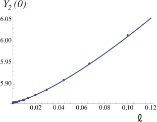
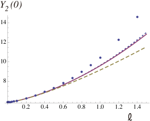
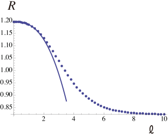
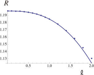
Figure 1 (a) shows a plot of $Y_{2}(0)$ as $\ell$ varies. As an example, the phase is fixed to be $\varphi=-\pi/20$ and the chemical potential to be $\mu=10$. We have chosen a real $\mu$ (imaginary $\phi$) so that we can compare our data against the three-loop result in term of the multiple polylogarithms [34] , which is discussed in the next section. Our expansions are valid also for real $\mu$. We find a good agreement between the numerical results and our analytic expansion. A fit by a function $\sum_{k=0}^{5}y_{2}^{(k)}l^{4k/3}$ for ${\cal O}(10^{-5})<\ell<{\cal O}(10^{-1})$ can also reproduce $Y_{2}^{(0,0)}$ and $Y_{2}^{(1,0)}$ with 12- and 8-digit accuracy, respectively. At ${\cal O}(l^{8/3})$, the coefficient $Y_{2}^{(2,0)}$ explains about 44 per cent of $y_{2}^{(2)}$, whereas about 51 per cent are from $Y_{2}^{(0,2)}$, which is determined by and proportional to $(Y_{2}^{(1,0)})^{2}$. The rest is carried by the undetermined $Y_{2}^{(1,1)}$. At ${\cal O}(l^{12/3})$, $Y_{2}^{(3,0)}$ explains about 16 per cent of $y_{2}^{(3)}$. Figure 1 (b) shows a plot of the expansions of $Y_{2}(0)$ obtained from the analytic data in the CFT limit, i.e., $Y_{2}^{(p,0)}$, up to $p=1,2,3$, respectively. $\varphi$ and $\mu$ are the same as in (a). Up to $\ell\sim 1$, the CFT data approximate $Y_{2}$ relatively well. Combining them with the Y-system yields better approximation.

(a)

(b)

Figure 1: Plot of $Y_{2}(0)$ for $\varphi=-\pi/20$ and $\mu=10$ as $\ell$ varies. In both (a) and (b), the points represent numerical results. In (a), the solid line represents the leading expansion (4.23) evaluated at $\theta=0$. (b) shows the expansions from the data in the CFT limit. The broken ($--$), solid $(-)$ and dotted ($\cdots$) lines represent $\sum_{p=0}^{k}2Y_{2}^{(p,0)}\cdot\ell^{4p\over 3}\cos\frac{4p}{3}\varphi$ with $k=1,2,3$, respectively. The case with $k=1$ is equivalent to (4.23).

5. Application to six-point amplitudes at strong coupling

Now, we apply the expansion of the Y-functions for small $\ell$ to the six-point amplitudes or the null-polygonal Wilson loops dual to the amplitudes. Our evaluation based on the quantum Wronskian relation allows us to analyze the amplitudes/Wilson loops corresponding to the minimal surfaces in AdS₅ or $\mu\neq 1$. In the small-$\ell$ or the UV limit, the Wilson loops become regular polygonal. The expansion thus gives the amplitudes/Wilson loops under small deformations around the regular polygonal contour.

To evaluate the amplitudes, we first recall that the remainder function in (2.26) consists of three terms. One of the terms denoted by $A_{\rm free}$ is nothing but the free energy of the ${\mathbb{Z}}_{4}$-symmetric integrable model twisted by $\phi$. Since this ${\mathbb{Z}}_{4}$-symmetric integrable model reduces, in the UV limit, to the twisted ${\mathbb{Z}}_{4}$-parafermion CFT, the free energy $A_{\rm free}$ is expanded by the bulk conformal perturbation theory [27]:

$$A_{\rm free} = \frac{\pi}{6}\Bigl{(}1-\frac{9\phi^{2}}{2\pi^{2}}\Bigr{)}-|Z|^{2}$$ (5.1)

$$\quad+\ 2\pi^{1/3}\kappa_{4}^{2}\gamma\Bigl{(}\frac{1}{3}\Bigr{)}\gamma\Bigl{(}\frac{1}{3}+\frac{\phi}{2\pi}\Bigr{)}\gamma\Bigl{(}\frac{1}{3}-\frac{\phi}{2\pi}\Bigr{)}\,|Z|^{\frac{8}{3}}+{\cal O}(|Z|^{\frac{16}{3}})\,,$$

where

$$\kappa_{4}=\frac{1}{2\pi}\gamma^{\frac{1}{2}}\Bigl{(}\frac{1}{6}\Bigr{)}\Bigl{[}\sqrt{\pi}\gamma\Bigl{(}\frac{3}{4}\Bigr{)}\Bigr{]}^{\frac{4}{3}}\,,$$ (5.2)

and $\gamma(z)=\Gamma(z)/\Gamma(1-z)$. The second term cancels $A_{\rm period}$.

The expansion of the remaining term $\Delta A_{\rm BDS}$ is derived by utilizing the results in (2.23), (2.24) and (2.26),

$$\Delta A_{\rm BDS}=-\frac{3}{4}\operatorname{Li}_{2}\bigl{(}1-U_{0}\bigr{)}+\frac{3\times 2^{\frac{2}{3}}(U_{0}-1+\log U_{0})}{U_{0}(U_{0}-1)^{2}}(Y_{2}^{(1,0)})^{2}|Z|^{\frac{8}{3}}+{\cal O}(|Z|^{\frac{16}{3}})\,.$$ (5.3)

Here, $U_{0}$ is the value of $U_{k}$ in the UV limit,

$$U_{0}=1+2Y_{2}^{(0,0)}=4\cos^{2}\bigl{(}{\phi}/{2}\bigr{)}\,,$$ (5.4)

common to all $k=1,2,3$. We note that $\Delta A_{\rm BDS}$ is expanded in powers of $Z^{4/3}=|Z|^{4/3}e^{i\frac{4}{3}\varphi}$ and its complex conjugate, but the $\varphi$-dependence remains only at ${\cal O}(|Z|^{8n/3})$ with $n\in 3{\mathbb{Z}}$. This is a consequence of the ${\mathbb{Z}}_{6}$-symmetry of the six-point amplitudes $\theta\to\theta+{\pi i}/{4}$ or $\varphi\to\varphi+{\pi}/{4}$, which corresponds to cyclically renaming the cusp points $x_{a}\to x_{a+1}$. This symmetry also explains the absence of the ${\cal O}(|Z|^{4/3})$ term.

Combining the above results, we obtain the UV expansion of the remainder function,

$$R=\sum_{k=0}^{\infty}r^{(k)}(\varphi,\phi)\,\ell^{\frac{8}{3}k}\,,$$ (5.5)

where

$$r^{(0)} = -\frac{\pi}{6}+\frac{3}{4\pi}\phi^{2}-\frac{3}{4}\operatorname{Li}_{2}\bigl{(}1-U_{0}\bigr{)}\,,$$

$$r^{(1)} = \frac{3\kappa_{4}^{2}}{32(2\pi)^{\frac{2}{3}}}\Bigl{[}\Bigl{(}1-\frac{8\sqrt{3}}{9}\Bigr{)}(1-U_{0})-\log U_{0}\Bigr{]}\cdot B^{2}\Bigl{(}\frac{1}{3}+\frac{\phi}{2\pi},\frac{1}{3}-\frac{\phi}{2\pi}\Bigr{)}\,,$$ (5.6)

and $B(x,y)$ is the beta function, $\Gamma(x)\Gamma(y)/\Gamma(x+y)$. The expansion of the Y-functions (4.23) also yields the cross-ratios for small $\ell$,

$$U_{k}=U_{0}+2Y_{2}^{(1,0)}\ell^{\frac{4}{3}}\cos\left[\frac{4}{3}\Bigl{(}\frac{2k+1}{4}\pi-\varphi\Bigr{)}\right]+{\cal O}(\ell^{\frac{8}{3}})\,.$$ (5.7)

Inverting this relation, one can express the parameters in the TBA equations by the cross-ratios [27],

$$\cos^{2}\frac{\phi}{2} = \frac{1}{12}(U_{1}+U_{2}+U_{3}),$$

$$\tan\frac{4}{3}\varphi = \frac{\sqrt{3}(U_{2}-U_{3})}{2U_{1}-U_{2}-U_{3}},$$ (5.8)

$$\ell^{\frac{4}{3}} = \frac{-2U_{1}+U_{2}+U_{3}}{6Y_{2}^{(1,0)}\cos\frac{4}{3}\varphi},$$

which is valid up to ${\cal O}(\ell^{\frac{8}{3}})$.

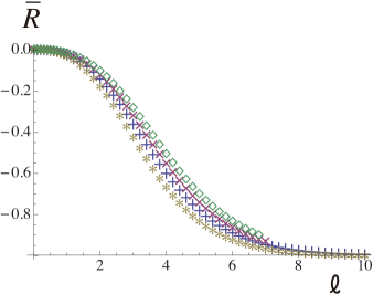
Our formulas can be checked numerically. Figure 2 (a) shows the trajectories of $u_{k}=1/U_{k}$ as $\ell$ varies with $\varphi$ and $\mu=e^{\frac{3}{2}i\phi}$ fixed to be $-\pi/20$ and $10$, respectively. They are obtained by solving the TBA equations and evaluating $A_{\rm free}$ numerically. Figure 2 (b) is a comparison of the same trajectories for small $\ell$ and the expansion of $u_{k}$ obtained from (5.7). Figure 3 (a) shows the remainder function at strong coupling $R$ for the cross-ratios $u_{k}$ given in Figure 2. The points represent the numerical results, whereas the solid line represents our expansion $R=r^{(0)}+r^{(1)}\ell^{8/3}$. Figure 3 (b) is the same plot for small $\ell$. From Figure 2 and 3, we find again a good agreement between the numerical results and our analytic expansions for small $\ell$.

(a)

(b)

Figure 2: (a) Trajectories of $u_{k}=1/U_{k}$ as $\ell$ varies with $\varphi=-\pi/20$ and $\mu=10$. Points denoted by $\ast,+,\times$ represent $u_{1},u_{2},u_{3}$, respectively. (b) The same trajectories for small $\ell$ (points) and the expansion from (5.7). The broken ($--$), solid $(-)$ and dotted ($\cdots$) lines represent $u_{1},u_{2},u_{3}$, respectively.

(a)

(b)

Figure 3: (a) Six-point reminder function at strong coupling as $\ell$ varies with $\varphi=-\pi/20$ and $\mu=10$. The points represent the numerical results, whereas the solid line represents our expansion (5.5) with (5.). (b) The same plot for small $\ell$.

6. Comparison with perturbative results

In [33, 20, 21, 22], the remainder functions of the strong-coupling amplitudes corresponding to the minimal surfaces in AdS₃ and AdS₄ were compared with the two-loop results. It was found there that after an appropriate normalization/rescaling they are close to each other. In this section, we compare the six-point remainder function at strong with those at two [48, 49], three [34] and four [10] loops.

For this purpose, we normalize/rescale the remainder function [33] so that it vanishes at $\ell=0$ and approaches $-1$ for large $\ell$:

$$\bar{R}^{\rm strong}={R^{\rm strong}-R^{\rm strong}_{\rm UV}\over R^{\rm strong}_{\rm UV}-R^{\rm strong}_{\rm IR}}\,,$$ (6.1)

where we have introduced the notation $R_{6}^{\rm strong}:=R$. $R^{\rm strong}_{\rm UV}$ ($R^{\rm strong}_{\rm IR}$) is the value at $\ell=0$ ($\ell=\infty$) along the trajectory in the space of the cross-ratios parametrized by $\ell$ with $\varphi,\mu$ fixed. For the remainder function at $L$ loops appearing in the perturbative expansion $R_{6}=\sum\lambda^{L}R^{(L)}$, one can also defined the rescaled reminder functions $\bar{R}^{(L)}$ similarly.

At strong coupling, the UV value is read off from the expansion in (5.5), $R^{\rm strong}_{\rm UV}=r^{(0)}$. To find the IR value $R^{\rm strong}_{\rm IR}$, we use the large-$\ell$ values of the cross-ratios $U_{k}\to(1,e^{\sqrt{2}\ell\cos(\frac{\pi}{4}+\varphi)},e^{\sqrt{2}\ell\cos(\frac{\pi}{4}-\varphi)})$, which are found from the Y-system (2.15), (2.16) and the asymptotic behavior $Y_{2}(\theta)\to 2\sqrt{2}(\bar{Z}e^{\theta}+Ze^{-\theta})$ for large $\ell$ with $|\,{\rm Im}\,\theta-\varphi|<\pi/2$. Since $A_{\rm free}\to 0$ and $A_{\rm period}$ cancels the leading term from $\Delta A_{\rm BDS}$ we are left with $R^{\rm strong}_{\rm IR}={\pi^{2}}/{12}$. On the perturbative side, $R_{\rm UV}^{(L)}$ are obtained from the cross-ratios $U_{0}$ in the UV limit, whereas the IR values just vanish $R_{\rm IR}^{(L)}=0$.

We evaluate these rescaled remainder functions for the cross-ratios $u_{k}(=1/U_{k})$ given in Figure 2, which are parametrized by $\ell$ with $\varphi=-\pi/20,\mu=10$. At strong coupling, it is readily read off from the results in the previous section. At two loops, we use the simple analytic expression given in [49], whereas at three loops we use the expression given in [34] and evaluate it by using the C++ library GiNaC [50, 51]. The direct three-loop expression in terms of the multiple polylogarithms is given for the parameter region with real $\mu$, which corresponds to the (2,2) signature of the four-dimensional space-time. In order to use this expression, we have chosen a real $\mu$. At four loops, it can be evaluated from the analytic expression in [10].

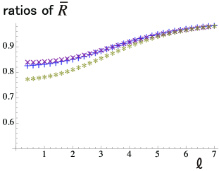
Figure 4 (a) is a plot of the rescaled remainder functions at two, three and four loops and at strong coupling. Figure 4 (b) is a plot of the ratios of these rescaled remainder functions; $\bar{R}^{(3)}/\bar{R}^{(2)}$, $\bar{R}^{(4)}/\bar{R}^{(3)}$ and $\bar{R}^{(2)}/\bar{R}^{\rm strong}$. As $\ell$ increases, it becomes harder to evaluate $R^{(3)}$ and Figure 4 includes the data for $\ell\leq 7$. It also includes the four-loop data for $\ell\leq 34/5$. Some of the numerical values of the rescaled remainder functions plotted in Figure 4 are listed in Table 1. From these figures and the table, we find that the rescaled remainder functions stay close to each other as $\ell$ varies, but the perturbative results gradually move away from those at strong coupling as the number of loops increases. Their ratios changes slowly along $\ell$, and accumulate to $1$ for large $\ell$ as assured by definition. The ratios of the perturbative results, $\bar{R}^{(3)}/\bar{R}^{(2)}$, $\bar{R}^{(4)}/\bar{R}^{(3)}$, are very similar. These are in accord with the observations in [33, 20, 21, 22] mentioned above and those in [34, 10] that the ratios of the remainder functions at two, three and four loops are relatively constant for large ranges of the cross-ratios.

As $\mu$ increases, we have observed that $\bar{R}_{6}^{(2)}$, $\bar{R}_{6}^{(3)}$ and $\bar{R}_{6}^{\rm strong}$ change in a similar manner: they tend to start decreasing for larger $\ell$. Although their differences increase, they are still kept relatively close to each other. The dependence on $\mu$ seems very weak. For example, even for $\mu=10^{6}$, the ratios are still of ${\cal O}(1)$. At the order of the expansion in (5.5) and (5.), the $\varphi$-dependence does not appear. Although it does appear at higher orders, the behavior of the rescaled remainder functions is still qualitatively similar.

(a)

(b)

Figure 4: (a) Rescaled remainder functions at two loops ($+$), three loops $(\times)$, four loops ($\diamond$) and strong coupling $(\ast)$ for the cross-ratios given in Figure 2 with $\varphi=-\pi/20$ and $\mu=10$. (b) Ratios of the rescaled remainder functions. Points denoted by $+,\times,\ast$ represent $\bar{R}^{(3)}/\bar{R}^{(2)}$, $\bar{R}^{(4)}/\bar{R}^{(3)}$ and $\bar{R}^{(2)}/\bar{R}^{\rm strong}$, respectively.

$\ell$	1/5	1	3	5	34/5	9	10
$\bar{R}^{(2)}$	$-3.202\times 10^{-4}$	-0.02351	-0.3618	-0.7814	-0.9388	-0.9890	-0.9951
$\bar{R}^{(3)}$	$-2.626\times 10^{-4}$	-0.01953	-0.3194	-0.7411	-0.9204	–	–
$\bar{R}^{(4)}$	$-2.214\times 10^{-4}$	-0.01643	-0.2827	-0.7014	-0.9004	–	–
$\bar{R}^{\rm strong}$	$-4.145\times 10^{-4}$	-0.03007	-0.4226	-0.8304	-0.9584	-0.9935	-0.9973

Table 1: Samples of the numerical values of the rescaled remainder functions plotted in Figure 4.

7. Conclusions

In this paper we studied six-point gluon scattering amplitudes in ${\cal N}=4$ super Yang-Mills theory at strong coupling by using the AdS/CFT correspondence. The area of the corresponding null-polygonal minimal surface in AdS₅ is evaluated by solving the T-/Y-system for the $\mathbb{Z}_{4}$-symmetric integrable model with a twist parameter. The leading expansion to the remainder function is determined around the UV limit explicitly. We compared this result with the recent perturbative calculations, to find that the rescaled remainder functions are close to each other along the trajectories parametrized by the scale parameter.

Our results at the leading order relied on the quantum Wronskian relation, which determines the expansion of the T-/Y-functions around the CFT (massless) limit. For higher order terms, one needs to study the massive TBA system intrinsically. As in [20, 21, 22], the boundary CPT would be a way toward this direction based on the relation between the T-/Y-functions and the $g$-function [28, 52, 53]. Through the T-/Y-functions, one could also study the quantum Wronskian relation from a different perspective by using the boundary CPT. However, it is yet to be figured out how to incorporate the twist of the perturbed $\mathbb{Z}_{4}$-parafermion theory in this framework.

Alternatively, the quantum Wronskian relation exists even in the massive case [46]. The more involved analyticity, however, defies the analytical determination of the moments of ${\bf A}$, $\bar{\bf A}$. Along [29, 28], the massive TBA systems have also been analyzed in [54, 55]. Hopefully one can detour the difficulties, and obtain the systematic higher expansions.

Finally, given the recent developments on the finite-coupling amplitudes around the collinear limit [12, 13, 14], it would be worthwhile to explore the extrapolation to the finite coupling also around the regular-polygonal limit. We hope to come back to these issues in near future.

Acknowledgements

We would like to thank Lance Dixon, James Drummond, Claude Duhr and Jeffrey Pennington for providing to us the four-loop data of the remainder function. We would also like to thank Lance Dixon and Takahiro Ueda for useful correspondences. The work of K. I., Y. S. and J. S. is supported in part by JSPS Grant-in-Aid for Scientific Research (C) No. 23540290, 24540248 and 24540399. The work of K. I. and Y. S. is also supported in part by JSPS Japan-Hungary Research Cooperative Program.

Appendix A. Non-Linear Integral Equation

We supplement a treatment on the Bethe ansatz equations based on suitably chosen auxiliary functions. The approach utilizes Non Linear Integral Equations satisfied by them[26, 56], and thus is referred to as the NLIE approach. Here we choose auxiliary functions as

$$\mathfrak{a}(x) =\frac{\Phi(x-i\frac{\gamma}{2}){\mathbf{Q}}(x+i\gamma)}{\Phi(x+i\frac{\gamma}{2}){\mathbf{Q}}(x-i\gamma)}, \mathfrak{A}(x) =1+\mathfrak{a}(x),$$

$$\bar{\mathfrak{a}}(x) =\frac{\Phi(x+i\frac{\gamma}{2}){\mathbf{Q}}(x-i\gamma)}{\Phi(x-i\frac{\gamma}{2}){\mathbf{Q}}(x+i\gamma)}, \bar{\mathfrak{A}}(x) =1+\bar{\mathfrak{a}}(x).$$

The Bethe ansatz equations are equivalent to

$$\mathfrak{a}(x_{j})=-1.$$

Numerically, one observes the following properties of the finite size system in the ground state:

1. $|\mathfrak{a}(x)|<1\,(|\bar{\mathfrak{a}}(x)|<1)$ in the upper (lower) half plane.

2. In a narrow strip including the real axis, the zeros of $\mathfrak{A}(x)\,(\bar{\mathfrak{A}}(x))$ are located only on the real axis and they coincide with the Bethe ansatz roots $\{x_{j}\}$.

3. The extended branch cut function, $\frac{1}{i}\ln\mathfrak{a}(x)$, is an increasing function of real $x$.

These properties are enough in deriving the NLIE. After the scaling and the conformal limit, for $\,{\rm Im}\,\theta$ positive small, it is explicitly given by

$$\ln\mathfrak{a}(\theta) =d_{a}(\theta)+\int_{-\infty+i0}^{\infty+i0}F(\theta-\theta^{\prime})\ln\mathfrak{A}(\theta^{\prime})\frac{d\theta^{\prime}}{2\pi}-\int_{-\infty-i0}^{\infty-i0}F(\theta-\theta^{\prime})\ln\bar{\mathfrak{A}}(\theta^{\prime})\frac{d\theta^{\prime}}{2\pi},$$

$$d_{a}(\theta) =i{\rm e}^{\theta}-i\frac{3\phi}{2},\qquad F(\theta)=-\int_{-\infty}^{\infty}\frac{{\rm e}^{ik\theta}}{2\cosh\frac{\pi}{2}k}dk,$$ (A.1)

where we use the same symbols $\mathfrak{a}$ etc for functions of $\theta(=\frac{3x}{2})$ by abuse of notation.

We are interested in $\phi\gg 1$ behavior of $\ln{\bf A}(\theta)$. The driving term $d_{a}$ in the above suggests that there exists $B$ of order $\ln\phi$ such that the smallest root $\theta_{1}$ is greater than $B$. We assume that $|\ln\mathfrak{A}(\theta)|\ll 1$ and $|\ln\bar{\mathfrak{A}}(\theta)|\ll 1$ if $\theta>\theta_{1}$. Introduce

$$g(\theta)=\ln\frac{\mathfrak{A}(\theta+B+i\epsilon)}{\bar{\mathfrak{A}}(\theta+B-i\epsilon)}.$$

Then for $\theta\leq 0$, the NLIE is approximated by the following Wiener-Hopf type equation [29],

$$g(\theta)=d_{a}(\theta+B)+\int_{-\infty}^{0}F(\theta-\theta^{\prime})g(\theta^{\prime})\frac{d\theta^{\prime}}{2\pi}.$$ (A.2)

It is convenient to deal with the equation in the Fourier space,

$$\widehat{g}(\omega)=\int_{-\infty}^{\infty}g(\theta){\rm e}^{-i\omega\theta}\frac{d\theta}{2\pi},\quad g(\theta)=\int_{-\infty}^{\infty}\widehat{g}(\omega){\rm e}^{i\omega\theta}d\omega.$$

The standard recipe is to introduce the factorized Kernel,

$$G_{+}(\omega)G_{-}(\omega)=\Bigl{(}1-\widehat{F}(\omega)\Bigr{)}^{-1},\qquad G_{-}(\omega)=G_{+}(-\omega)$$

such that

$$\lim_{\omega\rightarrow\infty}G_{\pm}(\omega)\rightarrow 1.$$

Explicitly we choose

$$G_{+}(\omega) =\sqrt{\frac{2\pi}{3}}\frac{\Gamma(1-\frac{3\omega}{4}i)}{\Gamma(\frac{1}{2}-\frac{\omega}{2}i)\Gamma(1-\frac{\omega}{4}i)}{\rm e}^{i\alpha\omega},$$

$$\alpha =\frac{1}{2}\Bigl{(}\ln\Bigl{(}\frac{3}{2}\Bigr{)}^{\frac{3}{2}}-\ln\Bigl{(}\frac{1}{2}\Bigr{)}^{\frac{1}{2}}\Bigr{)}.$$

Then the solution in the Fourier space is given as follows,

$$\widehat{g}(\omega) =G_{+}(\omega)\mathcal{Q}_{+}(\omega),$$

$$\mathcal{Q}_{+}(\omega) =\frac{1}{2\pi}\Bigl{(}\frac{3\phi}{2}\frac{G_{-}(-i\epsilon)}{\omega+i\epsilon}-\frac{G_{-}(-i)}{\omega+i}{\rm e}^{B}\Bigr{)}.$$

The comparison of the asymptotic behavior $\omega\rightarrow\infty$ of the Fourier transformation of (A.2) concludes $\mathcal{Q}_{+}(\infty)=0$. This determines the relation between parameters $B$ and $\phi$,

$${\rm e}^{B}=\frac{\phi}{2\sqrt{\pi}}\frac{\Gamma(\frac{1}{4})}{\Gamma(\frac{3}{4})}{\rm e}^{\alpha}.$$ (A.3)

This makes the expression for $\widehat{g}(\omega)$ simpler,

$$\widehat{g}(\omega)=\frac{i\phi\Gamma(1-\frac{3\omega}{4}i)}{2\sqrt{\pi}(\omega+i\epsilon)(\omega+i)\Gamma(\frac{1}{2}-\frac{\omega}{2}i)\Gamma(1-\frac{\omega}{4}i)}{\rm e}^{i\alpha\omega}.$$ (A.4)

We introduce $\mathbb{A}_{+}(\theta):=\ln\mathbf{A}(\theta+B)$ for $\theta<0$. A simple manipulation leads to the following expression of its Fourier transformation $\widehat{\mathbb{A}}_{+}(\omega)$ in terms of $\widehat{g}(\omega)$,

$$\widehat{\mathbb{A}}_{+}(\omega)=\frac{\widehat{g}(\omega)}{4\sinh\frac{\pi}{4}\omega\cosh\frac{\pi}{2}\omega}{\rm e}^{\frac{3\pi}{4}\omega}.$$ (A.5)

By substituting (A.4) into (A.5), one finds that $\omega=-\frac{4}{3}(n+1)i,n\in\mathbf{Z}_{\geq 0}$ are the only relevant poles in the inverse Fourier transformation of $\widehat{\mathbb{A}}_{+}(\omega)$. We thus finds for $\phi\gg 1$,

$$\ln\mathbf{A}(\theta)=-\frac{\phi}{4\sqrt{\pi}}\sum_{n\geq 1}{\rm e}^{\frac{2\gamma}{\pi}n(\alpha+\theta-B)}\frac{\Gamma(n(1-\frac{\gamma}{\pi}))\Gamma(\frac{1}{2}+\frac{\gamma}{\pi}n)}{(2\gamma n-\pi)n!}.$$

By comparing the above expansion with (4.10), making use of the explicit form of B in (A.3), we have the following asymptotic behavior of $a_{n}(\phi)$,

$$a_{n}(\phi)\sim\frac{\phi}{8\pi^{\frac{3}{2}}n!}\Gamma(\frac{n}{3})\Gamma(\frac{2n}{3}-\frac{1}{2})\Bigl{(}\frac{\phi}{2\sqrt{\pi}}\frac{\Gamma(\frac{1}{4})}{\Gamma(\frac{3}{4})}\Bigr{)}^{-\frac{4}{3}n}.$$

The explicit form of the coefficient $\alpha_{n}$ in (4.18) is then determined as in (4.19).

References

- [1] L. F. Alday and J. M. Maldacena, JHEP 0706 (2007) 064 [arXiv:0705.0303 [hep-th]].
- [2] J.M. Drummond, G.P. Korchemsky and E. Sokatchev, Nucl. Phys. B 795 (2008) 385 [arXiv:0707.0243 [hep-th]].
- [3] A. Brandhuber, P. Heslop and G. Travaglini, Nucl. Phys. B 794 (2008) 231 [arXiv:0707.1153 [hep-th]].
- [4] L. J. Mason and D. Skinner, JHEP 1012 (2010) 018 [arXiv:1009.2225 [hep-th]].
- [5] S. Caron-Huot, JHEP 1107 (2011) 058 [arXiv:1010.1167 [hep-th]].
- [6] J. M. Drummond, J. Henn, V. A. Smirnov and E. Sokatchev, JHEP 0701 (2007) 064 [arXiv:hep-th/0607160].
- [7] J.M. Drummond, J. Henn, G.P. Korchemsky and E. Sokatchev, Nucl. Phys. B 826 (2010) 337 [arXiv:0712.1223 [hep-th]].
- [8] J. M. Drummond, J. Henn, G. P. Korchemsky and E. Sokatchev, Nucl. Phys. B 828 (2010) 317 [arXiv:0807.1095 [hep-th]].
- [9] Z. Bern, L. J. Dixon and V. A. Smirnov, Phys. Rev. D 72, 085001 (2005) [arXiv:hep-th/0505205].
- [10] L. J. Dixon, J. M. Drummond, C. Duhr and J. Pennington, arXiv:1402.3300 [hep-th].
- [11] L. F. Alday, D. Gaiotto, J. Maldacena, A. Sever and P. Vieira, JHEP 1104 (2011) 088 [arXiv:1006.2788 [hep-th]].
- [12] B. Basso, A. Sever and P. Vieira, Phys. Rev. Lett. 111 (2013) 091602 [arXiv:1303.1396 [hep-th]].
- [13] B. Basso, A. Sever and P. Vieira, JHEP 1401 (2014) 008 [arXiv:1306.2058 [hep-th]].
- [14] B. Basso, A. Sever and P. Vieira, arXiv:1402.3307 [hep-th].
- [15] L. F. Alday and J. Maldacena, JHEP 0911 (2009) 082 [arXiv:0904.0663 [hep-th]].
- [16] L. F. Alday, D. Gaiotto and J. Maldacena, JHEP 1109 (2011) 032. arXiv:0911.4708 [hep-th].
- [17] L. F. Alday, J. Maldacena, A. Sever and P. Vieira, J. Phys. A 43 (2010) 485401 [arXiv:1002.2459 [hep-th]].
- [18] Y. Hatsuda, K. Ito, K. Sakai and Y. Satoh, JHEP 1004 (2010) 108 [arXiv:1002.2941 [hep-th]].
- [19] C. R. Fernandez-Pousa, M. V. Gallas, T. J. Hollowood, J. L. Miramontes, Nucl. Phys. B 484 (1997) 609 [arXiv:hep-th/9606032].
- [20] Y. Hatsuda, K. Ito, K. Sakai and Y. Satoh, JHEP 1104, 100 (2011) [arXiv:1102.2477 [hep-th]].
- [21] Y. Hatsuda, K. Ito and Y. Satoh, JHEP 1202, 003 (2012) [arXiv:1109.5564 [hep-th]].
- [22] Y. Hatsuda, K. Ito and Y. Satoh, JHEP 1302, 067 (2013) [arXiv:1211.6225 [hep-th]].
- [23] R. Koberle and J. A. Swieca, Phys. Lett. B 86 (1979) 209.
- [24] A. M. Tsvelick, Nucl. Phys. B 305 [FS23] (1988) 675.
- [25] V. A. Fateev, Int. J. Mod. Phys. A 6 (1991) 2109.
- [26] A. Klümper, M. T. Batchelor and P. A. Pearce, J. Phys. A 24 (1991) 3113.
- [27] Y. Hatsuda, K. Ito, K. Sakai and Y. Satoh, JHEP 1009 (2010) 064 [arXiv:1005.4487 [hep-th]].
- [28] V. V. Bazhanov, S. L. Lukyanov and A. B. Zamolodchikov, Commun. Math. Phys. 177 (1996) 381 [hep-th/9412229].
- [29] V. V. Bazhanov, S. L. Lukyanov and A. B. Zamolodchikov, Commun. Math. Phys. 190 (1997) 247 [hep-th/9604044].
- [30] V. V. Bazhanov, S. L. Lukyanov and A. B. Zamolodchikov, Nucl. Phys. B549 (1999) 529-545 [arXiv:hep-th/9812091].
- [31] P. Dorey, C. Dunning and R. Tateo, J. Phys. A 40 (2007) R205 [arXiv:hep-th/0703066].
- [32] N. Gromov, V. Kazakov, S. Leurent and Z. Tsuboi, JHEP 1101 (2011) 155 [arXiv:1010.2720 [hep-th]].
- [33] A. Brandhuber, P. Heslop, V. V. Khoze and G. Travaglini, JHEP 1001 (2010) 050 [arXiv:0910.4898 [hep-th]].
- [34] L. J. Dixon, J. M. Drummond, M. von Hippel and J. Pennington, JHEP 1312 (2013) 049 [arXiv:1308.2276 [hep-th]].
- [35] B. Basso, A. Sever and P. Vieira, arXiv:1405.6350 [hep-th].
- [36] Al. B. Zamolodchikov, Nucl. Phys. B 342 (1990) 695.
- [37] J. Bartels, J. Kotanski and V. Schomerus, JHEP 1101 (2011) 096 [arXiv:1009.3938 [hep-th]].
- [38] J. Bartels, J. Kotanski, V. Schomerus and M. Sprenger, arXiv:1311.1512 [hep-th].
- [39] C. Destri and H. J. de Vega, Nucl. .Phys. B290 (1987) 363-391.
- [40] R. J. Baxter, Ann .Phys. (N.Y.)70 (1972) 193-228.
- [41] A. B. Zamolodchikov, Phys. Lett. B 253 (1991) 391.
- [42] S. Fomin and A. Zelevinsky, Ann. Math. 158 (2003) 977-1018.
- [43] B. Keller, arXiv:0807.1960.
- [44] R. Inoue, O. Iyama, B. Keller, A. Kuniba , T. Nakanishi, Publ. RIMS. 49 (2013) 1-42.
- [45] R. Inoue, O. Iyama, B. Keller, A. Kuniba , T. Nakanishi, Publ. RIMS. 49 (2013) 43-85.
- [46] S. L. Lukyanov and A. B. Zamolodchikov, JHEP 07 (2010) 008 [arXiv:1003.5333 [hep-th]].
- [47] G. P. Pronko and Yu. G. Stroganov, J. Phys. A: Mathemaical and General 32 (2010) 2333 [hep-th/9808153].
- [48] V. Del Duca, C. Duhr and V. A. Smirnov, JHEP 1005 (2010) 084 [arXiv:1003.1702 [hep-th]].
- [49] A. B. Goncharov, M. Spradlin, C. Vergu and A. Volovich, Phys. Rev. Lett. 105 (2010) 151605 [arXiv:1006.5703 [hep-th]].
- [50] C. W. Bauer, A. Frink and R. Kreckel, cs/0004015 [cs-sc].
- [51] J. Vollinga and S. Weinzierl, Comput. Phys. Commun. 167 (2005) 177 [hep-ph/0410259].
- [52] P. Dorey, I. Runkel, R. Tateo and G. Watts, Nucl. Phys. B 578 (2000) 85 [arXiv:hep-th/9909216].
- [53] P. Dorey, A. Lishman, C. Rim and R. Tateo, Nucl. Phys. B 744 (2006) 239 [hep-th/0512337].
- [54] V. V. Bazhanov, S. L. Lukyanov and A. B. Zamolodchikov, Nucl. Phys. B 489 (1997) 487 [arXiv:hep-th/9607099].
- [55] D. Fioravanti and M. Rossi, JHEP 0308 (2003) 042 [arXiv:hep-th/0302220].
- [56] C. Destri and H. J. de Vega, Phys. Rev. Lett. 69 (1992) 2313.