Blind Sensor Calibration using Approximate Message Passing

Abstract

The ubiquity of approximately sparse data has led a variety of communities to great interest in compressed sensing algorithms. Although these are very successful and well understood for linear measurements with additive noise, applying them on real data can be problematic if imperfect sensing devices introduce deviations from this ideal signal acquisition process, caused by sensor decalibration or failure. We propose a message passing algorithm called calibration approximate message passing (Cal-AMP) that can treat a variety of such sensor-induced imperfections. In addition to deriving the general form of the algorithm, we numerically investigate two particular settings. In the first, a fraction of the sensors is faulty, giving readings unrelated to the signal. In the second, sensors are decalibrated and each one introduces a different multiplicative gain to the measurements. Cal-AMP shares the scalability of approximate message passing, allowing to treat big sized instances of these problems, and experimentally exhibits a phase transition between domains of success and failure.

1 Introduction

Compressed sensing (CS) has made it possible to algorithmically invert an underdetermined linear system, provided that the signal to recover is sparse enough and that the mixing matrix has certain properties [1]. In addition to the theoretical interest raised by this discovery, CS is already used both in experimental research and in real world applications, in which it can lead to significant improvements. CS is particularly attractive for technologies in which an increase of the number of measurements is either impossible, as sometimes in medical imaging [2, 3], or expensive, as in imaging devices that operate in certain wavelength [4]. CS was extended to the setting in which the mixing process is followed by a sensing process which can be nonlinear or probabilistic, as shown in Fig. 1, with an algorithm called the generalized approximate message passing (GAMP) [5]. This has opened new applications of CS, such as phase retrieval [6].

Figure 1: The generalized compressed sensing setting in GAMP [5]: the mixing step is followed by a sensing step, characterized by the probability distribution $p_{Y|Z}$.

Figure 2: The blind calibration problem: the sensing process is known up to calibration parameters $\mathbf{d}$ that need to be recovered jointly with the signal. For this to be possible, one generally needs to measure $P>1$ independent signals. Note that the elements of $\mathbf{d}$ are characteristic of the sensing system and therefore do not depend on the signal measured.

One issue that can arise in CS is a lack of knowledge or an uncertainty on the exact measurement process. A known example is dictionary learning, where the measurement matrix $\mathbf{F}$ is not known. The dictionary learning problem can also be solved with an AMP-based algorithm if the number $P$ of available signal samples grows as $N$ [7].

A different kind of uncertainty is when the linear transformation $\mathbf{F}$, corresponding to the mixing process, is known, but the sensing process is only known up to a set of parameters. In some cases, it might be possible to estimate these parameters prior to the measurements in a supervised sensor calibration process, during which one measures the outputs produced by known training signals, and in this way estimate the parameters for each of the sensors. In other cases, this might not be possible or practical, and the parameters have to be estimated jointly with a set of unknown signals: this is known as the blind sensor calibration problem. It is schematically shown on Fig. 2.

Some examples in which supervised calibration is impossible are given here:

• For supervised calibration to be possible, one must be able to measure a known signal. This might not always be the case: in radio astronomy for example, calibration is necessary [8], but the only possible observation is the sky, which is only partially known.

• Supervised calibration is only possible when the system making the measurements is at hand, which might not always be the case. Blind image deconvolution is an example of blind calibration in which the calibration parameters are the coefficients of the imaging device’s point spread function. It can easily be measured, but if we only have the blurred images and not the camera, there is no other option than estimating the point spread function from the images themselves, thus performing blind calibration [9].

• For measurement systems integrated in embedded systems or smartphones, requiring a supervised calibration step before taking a measurement might be possible, but is not user-friendly because it requires a specific calibration procedure, which blind calibration does not. On the other hand, regular calibration might be necessary, as slow decalibration can occur because of aging or external parameters such as temperature or humidity.

Several algorithms have been proposed for blind sensor calibration in the case of unknown multiplicative gains, relying on convex optimization [10] or conjugate gradient algorithms [11]. The Cal-AMP algorithm that we propose, and whose preliminary study was presented in [12], is based on GAMP and is therefore not restricted to a specific output function. Furthermore, it has the same advantages in speed and scalability as the approximate message passing (AMP), and thus allows to treat problems with big signal sizes.

2 Blind sensor calibration: Model and notations

2.1 Notations

In the following, vectors and matrices will be written using bold font. The $i$-th component of the vector $\mathbf{a}$ will be written as $a_{i}$. In a few cases, notations of the type $\mathbf{a}_{i}$ are used, in which case $\mathbf{a}_{i}$ is a vector itself, not the $i$-th component of vector $\mathbf{a}$. The complex conjugate of a complex number $x\in\mathbb{C}$ will be noted $x^{*}$, and its modulo $|x|$. The transpose (resp. complex transpose) of a real (resp. complex) vector $\mathbf{x}$ will be noted $\mathbf{x}^{T}$. The component-wise product between two vectors or matrices $\mathbf{a}$ and $\mathbf{b}$ will be noted $\mathbf{a}\odot\mathbf{b}$. The notations $\mathbf{a}^{-1}$, and $\frac{\mathbf{b}}{\mathbf{a}}$ are component-wise divisions, and $\mathbf{a}^{2}=\mathbf{a}\odot\mathbf{a}$. We will call a probability distribution function (pdf) on a matrix or vector variable $\mathbf{a}$ separable if its components are independently distributed: $p(\mathbf{a})=\prod_{i}p(a_{i})$. Finally, we will write $p(x)\propto f(x)$ if $p$ and $f$ are proportional and we will write $x\sim p_{X}(x)$ if $x$ is a random variable with probability distribution function $p_{X}$.

2.2 Measurement process

Let $\mathbf{x}$ be a set of $P$ signals $\{\mathbf{x}_{l},l=1\cdots P\}$ to be recovered and $N$ be their dimension: $\mathbf{x}_{l}\in\mathbb{R}^{N}$. Each of those signals is sparse, meaning that only a fraction $\rho$ of their components is non-zero.

The measurement process leading to $\mathbf{y}\in\mathbb{R}^{M\times P}$ is shown in Fig. 2. In the first, linear step, the signal is multiplied by a matrix $\mathbf{F}\in\mathbb{R}^{M\times N}$ and gives a variable $\mathbf{z}\in\mathbb{R}^{M\times P}$

$$\mathbf{z} =\mathbf{F}\mathbf{x},$$ (1)

or, written component-wise

$$z_{\mu l} =\sum_{i=1}^{N}F_{\mu i}x_{il}\quad\quad{\rm for}\quad\mu=1\cdots M,\quad l=1\cdots P.$$ (2)

We will refer to $\alpha={M}/{N}$ as the measurement rate. In standard CS, the measurement $\mathbf{y}$ is a noisy version of $\mathbf{z}$, and the goal is to reconstruct $\mathbf{x}$ in the regime where the rate $\alpha<1$. In the broader GAMP formalism, $\mathbf{z}$ is only an intermediary variable that cannot directly be observed. The observation $\mathbf{y}$ is a function of $\mathbf{z}$, which is probabilistic in the most general setting.

In blind calibration, we add the fact that this function depends on an unknown parameter vector $\mathbf{d}\in\mathbb{R}^{M}$, such that the output function of each sensor is different,

$$\mathbf{y}\sim p_{\mathbf{Y}|\mathbf{Z},\mathbf{D}}(\mathbf{y}|\mathbf{z},\mathbf{d}),$$ (3)

with

$$p_{\mathbf{Y}|\mathbf{Z},\mathbf{D}}(\mathbf{y}|\mathbf{z},\mathbf{d}) =\prod_{\mu=1}^{M}\prod_{l=1}^{P}p_{Y|Z,D}(y_{\mu l}|z_{\mu l},d_{\mu}),$$ (4)

and the goal is to jointly reconstruct $\mathbf{x}$ and $\mathbf{d}$.

2.3 Properties AMP for compressed sensing

It is useful to remind basic results known about the AMP algorithm for compressed sensing [13]. The AMP is derived on the basis of belief propagation [14]. As is well known, belief propagation on a loopy factor graph is not in general guaranteed to give sensible results. However, in the setting of this paper, i.e. random iid matrix $\mathbf{F}$ and signal with random iid elements of known probability distribution, the AMP algorithm was proven to work in compressed sensing in the the limit of large system size $N$ as long as the measurement rate $\alpha\geq\alpha_{\rm CS}(\rho)$ [13, 15, 16, 17]. The threshold $\alpha_{\rm CS}(\rho)$ is a phase transition, meaning that in the limit of large system size, AMP fails with high probability up to the threshold $\alpha_{\rm CS}(\rho)\in(\rho,1)$ and succeeds with high probability above that threshold.

2.4 Technical conditions

The technical conditions necessary for the derivation of the Cal-AMP algorithm and its good behavior are the following:

• Ideally, the prior distributions of both the signal, $p_{\mathbf{X}}$, and the calibration parameters, $p_{\mathbf{D}}$, are known, such that we can perform Bayes-optimal inference. As in CS, a mismatch between the real distribution and the assumed prior will in general affect the performance of the algorithm. However, parameters of the real distribution can be learned with expectation-maximization and improve performance [17].

• The Cal-AMP can be tested for an arbitrary operator $\mathbf{F}$. However, in its derivation we assume that $\mathbf{F}$ is an iid random matrix, and that its elements are of order $O(\frac{1}{\sqrt{N}})$, such that $\mathbf{z}$ is $O(1)$ (given that $\mathbf{x}$ is $O(1)$). The mean of elements of $\mathbf{F}$ should be close to zero for the AMP-algorithms to be stable, in the opposite case the implementation has to be adjusted by some of the methods known to fix this issue [18].

• The output function $p_{\mathbf{Y}|\mathbf{Z},\mathbf{D}}$ has to be separable, as well as the priors on $\mathbf{x}$ and $\mathbf{d}$. This condition could be relaxed by using techniques similar to those allowing to treat the case of structured sparsity in [19].

Under the above conditions we conjecture that in the limit of large system sizes the Cal-AMP algorithm matches the performance of the Bayes-optimal algorithm (except in a region of parameters where the Bayes-optimal fixed point of the Cal-AMP is not reached from an non-informed initialization, the same situation was described in compressed sensing [17]). This conjecture is based on the insight from the theory of spin glasses [20], and it makes the Cal-AMP algorithm stand out among other possible extensions of GAMP that would take into account estimation of the distortion parameters. Proof of this conjecture is a non-trivial challenge for future work.

2.5 Relation to GAMP and some of its existing extensions

Cal-AMP algorithm can be seen as an extension of GAMP [5].

Cal-AMP reduces to GAMP for the particular case of a single signal sample $P=1$. Indeed, if the measurement $y_{\mu}$ depends on a parameter $d_{\mu}$ via a probability distribution function $p_{Y|Z,D}$, then $p_{Y|Z}$ can be expressed by:

$$p_{Y|Z}(y_{\mu}|z_{\mu})=\int{\rm d}d_{\mu}p_{D}(d_{\mu})p_{Y|Z,D}(y_{\mu}|z_{\mu},d_{\mu})\,.$$ (5)

When, however, the number of signal samples is greater than one, $P>1$, the two algorithms differ: while GAMP treats the $P$ signals independently, leading to the same reconstruction performances no matter the value of $P$, Cal-AMP treats them jointly. As our numerical results show, this can lead to great improvements in reconstruction performances, and can allow exact signal reconstruction in conditions under which GAMP fails.

One work on blind calibration that used a GAMP-based algorithm is [21], where the authors combine GAMP with expectation maximization-like learning. That paper, however, considers a setting different from ours in the sense that the unknown gains are on the signal components not on the measurement components. Whereas both these cases are relevant in practice, from an algorithmic point of view they are different.

Another work where distortion-like parameters are included and estimated with a GAMP-based algorithm is [22, 23]. Authors of this work consider two types of distortion-like parameters. Parameters $S$ that are sample-dependent and hence their estimation is more related to what is done in the matrix factorization problem rather than to the blind calibration considered here. And binary parameters $b$ that are estimated independently of the main loop that uses GAMP. The problem considered in that work requires a setting and a factor graph more complex that the one we considered here and it is far from transparent what to conclude about performance for blind calibration from the results presented in [22, 23].

3 The Cal-AMP algorithm

In this section, we give details of the derivation of the approximate message passing algorithm for the calibration problem (Cal-AMP). It is closely related to the AMP algorithm for CS [13] and the derivation was made using the same strategy as in [17]. First, we express the blind sensor calibration problem as an inference problem, using Bayes’ rule and an a priori knowledge of the probability distribution functions of both the signal and the calibration parameters. From this, we obtain an a posteriori distribution, which is peaked around the unique solution with high probability. We write belief propagation equations that lead to an iterative update procedure of signal estimates. We realize that in the limit of large system size the algorithm can be simplified by working only with the means and variances of the corresponding messages. Finally, we reduce the computational complexity of the algorithm by noting that the messages are perturbed versions of the local beliefs, which become the only quantities that need updating.

3.1 Probabilistic approach and belief propagation

We choose a probabilistic approach to solve the blind calibration problem, which has been shown to be very successful in CS. The starting point is Bayes’ formula that allows us to estimate the signal $\mathbf{x}$ and the calibration parameters $\mathbf{d}$ from the knowledge of the measurements $\mathbf{y}$ and the measurement matrix $\mathbf{F}$, assuming that $\mathbf{x}$ and $\mathbf{d}$ are statistically independent,

$$p(\mathbf{x},\mathbf{d}|\mathbf{y},\mathbf{F}) =\frac{p_{\mathbf{X}}(\mathbf{x})p_{\mathbf{D}}(\mathbf{d})p(\mathbf{y}|\mathbf{F},\mathbf{x},\mathbf{d})}{p(\mathbf{y}|\mathbf{F})}.$$ (6)

Using separable priors on $\mathbf{x}$ and $\mathbf{d}$ as well as separable output functions, this posterior distribution becomes

$$p(\mathbf{x},\mathbf{d}|\mathbf{y},\mathbf{F})=\frac{1}{Z} \prod_{i,l=1}^{N,P}p_{X}({x}_{il})\prod_{\mu=1}^{M}p_{D}({d}_{\mu})\times$$

$$\prod_{l,\mu=1}^{P,M}p_{Y|Z,D}({y}_{\mu l}|{z}_{\mu l},{d}_{\mu}),$$ (7)

where $Z$ is the normalization constant. Even in the factorized form of (7), uniform sampling from this posterior distribution becomes intractable with growing $N$.

Representing (7) by the factor graph in Fig. 3 allows us to use belief propagation for approximate sampling. As the factor graph is not a tree, there is no guarantee that running belief propagation on it will lead to the correct results. Relying on the success of AMP in compressed sensing and the insight from the theory of spin glasses [20], we conjecture belief propagation to be asymptotically exact in blind calibration as it is in CS.

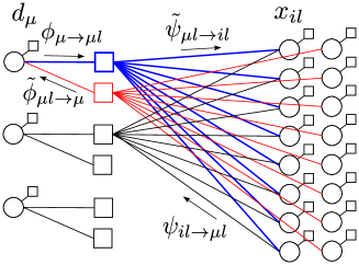
Figure 3: Graphical model representing the posterior distribution (7) of the blind calibration problem. Here, the dimension of the signal is $N\!=\!8$, the number of sensors is $M\!=\!3$, and the number of signals used for calibration $P\!=\!2$. The variable nodes $x_{il}$ and $d_{\mu}$ are depicted as circles, the factor nodes as squares (for clarity, only the three upper factor nodes are represented with all their links).

In belief propagation there are two types of pairs of messages: $(\psi,\tilde{\psi})$ and $(\phi,\tilde{\phi})$, connected to the signal components and to the calibration parameters respectively. Their updating scheme in the sum-product belief propagation is the following [14]: for the $(\phi,\tilde{\phi})$ messages,

$$\phi_{\mu\to\mu l}^{t}({d}_{\mu}) \propto p_{D}({d_{\mu}})\prod_{m\neq l}\tilde{\phi}_{\mu m\to\mu}^{t}({d}_{\mu}),$$ (8)

$$\tilde{\phi}_{\mu l\to\mu}^{t+1}({d}_{\mu}) \propto\int\left(\prod_{i}{\rm d}{x}_{il}\psi_{il\to\mu l}^{t}({x}_{il})\right)\times$$

$$p_{Y|Z,D}({y}_{\mu l}|\sum_{i}{F}_{\mu i}{x}_{il},{d}_{\mu}),$$ (9)

whereas for the $(\psi,\tilde{\psi})$ messages,

$$\psi_{il\to\mu l}^{t}({x}_{il}) \propto p_{X}({x}_{il})\prod_{\gamma\neq\mu}\tilde{\psi}_{\gamma l\to il}^{t}({x}_{il}),$$ (10)

$$\tilde{\psi}_{\mu l\to il}^{t+1}({x}_{il}) \propto\int{\rm d}{d}_{\mu}\phi_{\mu\to\mu l}^{t}({d}_{\mu})\int\left(\prod_{j\neq i}{\rm d}{x}_{jl}\psi_{jl\to\mu l}^{t}({x}_{jl})\right)\times$$

$$p_{Y|Z,D}({y}_{\mu l}|\sum_{i}{F}_{\mu i}{x}_{il},{d}_{\mu}).$$ (11)

When belief propagation is successful, these messages converge to a fixed point, from which we obtain the marginal distribution of $\mathbf{x}$ sampled with (7):

$$\psi_{il}^{t} \propto p_{X}(x_{il})\prod_{\gamma}\tilde{\psi}_{\gamma l\to il}^{t}(x_{il}).$$ (12)

These distributions are called beliefs, and from them we obtain the minimal mean square error (MMSE) estimator:

$$\hat{x}_{il}^{\rm MMSE}=\int{\rm d}x_{il}\,x_{il}\psi_{il}(x_{il}).$$ (13)

3.2 Simplifications in the large $N$ limit

The above update equations are still intractable, given the fact that in general, $x_{il}$ and $d_{\mu}$ are continuous variables. In the large $N$ limit, the problem can be greatly simplified by making leading-order expansions of certain quantities as a function of the matrix elements $F_{\mu i}$, that are of order $1/\sqrt{N}$. The notation $O(F_{\mu i})$ is therefore equivalent to $O(1/\sqrt{N})$.

This allows to pass messages that are estimators of variables and of their uncertainty, instead of full probability distributions. The table in Fig. 4 is a summary of notations used and their significations: estimators of variables are noted with a hat, whereas their uncertainties are noted with a bar.

variable	$x$		$z$		$d$
mean	$\hat{X}$	$\hat{x}$	$\hat{Z}$	$\hat{z}$	$\hat{D}$	$\hat{d}$
variance	$\bar{X}$	$\bar{x}$	$\bar{Z}$	$\bar{z}$	$\bar{D}$	$\bar{d}$

Figure 4: Notations of the estimators and uncertainty estimators of the variables to be inferred. Upper case letters represent estimations obtained from the most recent estimates of the other variables, lower case letters are estimates taking into account the prior (for $x$ and $d$) and the data (for $z$).

The messages can then be expressed in simpler ways by using Gaussians. As these will be ubiquitous in the rest of the paper, let us introduce the notation

$$\mathcal{N}({x};{R},{\Sigma}) =\frac{e^{-\frac{(x-R)^{2}}{2\Sigma}}}{\sqrt{2\pi\Sigma}},$$ (14)

and note the expression of the following derivative:

$$\frac{\partial}{\partial R}\mathcal{N}(x;R,\Sigma) =\frac{x-R}{\Sigma}\mathcal{N}(x;R,\Sigma).$$ (15)

We will also use convolutions of a function $g$, with optional parameters $\{u\}$, with a Gaussian

$$f_{k}^{g}(R,\Sigma,\{u\}) =\int{\rm d}x\,x^{k}g(x,\{u\})\mathcal{N}(x;R,\Sigma),$$

$$\hat{f}^{g}(R,\Sigma,\{u\}) =\frac{f_{1}^{g}(R,\Sigma,\{u\})}{f_{0}^{g}(R,\Sigma,\{u\})},$$ (16)

$$\bar{f}^{g}(R,\Sigma,\{u\}) =\frac{f_{2}^{g}(R,\Sigma,\{u\})}{f_{0}^{g}(R,\Sigma,\{u\})}-|\hat{f}^{g}(R,\Sigma,\{u\})|^{2},$$

and from (15), we obtain the relations

$$\frac{\partial}{\partial R}f_{k}^{g}(R,\Sigma,\{u\}) =\frac{f_{k+1}^{g}(R,\Sigma,\{u\})-Rf_{k}^{g}(R,\Sigma,\{u\})}{\Sigma},$$ (17)

$$\Sigma\,\frac{\partial}{\partial R}\hat{f}^{g}({R},{\Sigma},\{u\}) =\bar{f}^{g}({R},{\Sigma},\{u\}).$$

Let us show how simplifications come about in the large $N$ limit. Both in (9) and in (11), the term $p_{Y|Z,D}(y_{\mu l}|z_{\mu l}=\sum_{i}F_{\mu i}x_{il},d_{\mu})$ appears. $z_{\mu l}$ is a sum of the $N$ random variables $F_{\mu i}x_{il}$, and each $x_{il}$ is distributed according to the distribution $\psi_{il\to\mu l}^{t}(x_{il})$. Let us call $\hat{x}_{il\to\mu l}$ and $\bar{x}_{il\to\mu l}$ the means and variances of these distributions,

$${\hat{x}}_{il\to\mu l}^{t} =\int{\rm d}x_{il}\,{x}_{il}\psi_{il\rightarrow\mu l}^{t}({x_{il}}),$$ (18)

$${\bar{x}}_{il\to\mu l}^{t} =\int{\rm d}x_{il}\,{x}_{il}^{2}\psi_{il\rightarrow\mu l}^{t}({x_{il}})-({\hat{x}}^{t}_{il\to\mu l})^{2}.$$ (19)

In the $N\to\infty$ limit, we can use the central limit theorem, as the assumption of independence of the variables is already made when writing the belief propagation equations. Then, $z_{\mu l}$ has a normal distribution with means and variances:

$${\hat{Z}}_{\mu l}^{t+1} =\sum_{i}{F}_{\mu i}{\hat{x}}_{il\to\mu l}^{t},$$ (20)

$${\bar{Z}}_{\mu l}^{t+1} =\sum_{i}{F}_{\mu i}^{2}{\bar{x}}_{il\to\mu l}^{t}.$$ (21)

In (9) we therefore obtain

$$\tilde{\phi}_{\mu l\to\mu}^{t+1}(d_{\mu}) \propto\int{\rm d}z_{\mu l}\mathcal{N}(z_{\mu l};\hat{Z}_{\mu l}^{t+1},\bar{Z}_{\mu l}^{t+1})p_{Y|Z,D}(y_{\mu l}|z_{\mu l},d_{\mu})$$

$$\propto f_{0}^{Z}(\hat{Z}_{\mu l}^{t+1},\bar{Z}_{\mu l}^{t+1},y_{\mu l},d_{\mu}),$$ (22)

where $f_{0}^{Z}(\hat{Z},\bar{Z},y,d)$ is a lighter notation for $f_{0}^{p_{Y|Z,D}}(\hat{Z},\bar{Z},\{y,d\})$ given by the formula in (16).

For the $\phi$ messages, we obtain that

$$\phi_{\mu\to\mu l}^{t}(d_{\mu})\propto p_{D}(d_{\mu})\prod_{m\neq l}f_{0}^{Z}(\hat{Z}_{\mu m}^{t},\bar{Z}_{\mu m}^{t},y_{\mu m},d_{\mu}).$$ (23)

The same procedure can be applied to the $\tilde{\psi}$ messages, the only difference being that $x_{il}$ is fixed, leading to

$$\tilde{\psi}_{\mu l\to il}^{t+1}({x}_{il}) \propto\int{\rm d}{d}_{\mu}f_{0}^{Z}(\hat{Z}_{\mu l\to il}^{t+1}+F_{\mu i}x_{il},\bar{Z}_{\mu l\to il}^{t+1},y_{\mu l},d_{\mu})\times$$

$$p_{D}({d}_{\mu})\prod_{m\neq l}f_{0}^{Z}(\hat{Z}_{\mu m}^{t},\bar{Z}_{\mu m}^{t},y_{\mu m},d_{\mu}),$$ (24)

with

$${\hat{Z}}_{\mu l\to il}^{t+1} =\sum_{j\neq i}{F}_{\mu j}{\hat{x}}_{jl\to\mu l}^{t},$$ (25)

$${\bar{Z}}_{\mu l\to il}^{t+1} =\sum_{j\neq i}{F}_{\mu j}^{2}{\bar{x}}_{jl\to\mu l}^{t}.$$ (26)

In analogy to the functions defined in (16), we introduce the functions of the $P$-dimensional vectors $\mathbf{\mathbf{\hat{Z}}}$, $\mathbf{\mathbf{\bar{Z}}}$ and $\mathbf{y}$:

$$g_{k}(\mathbf{\hat{Z}},\mathbf{\bar{Z}},\mathbf{y}) =\int{\rm d}d_{\mu}p_{D}(d_{\mu})f_{k}^{Z}(\hat{Z}_{1},\bar{Z}_{1},y_{1},d_{\mu})\times$$

$$\prod_{m=2}^{P}f_{0}^{Z}(\hat{Z}_{m},\bar{Z}_{m},y_{m},d_{\mu}),$$

$$\hat{g}(\mathbf{\hat{Z}},\mathbf{\bar{Z}},\mathbf{y}) =\frac{g_{1}(\mathbf{\hat{Z}},\mathbf{\bar{Z}},\mathbf{y})}{g_{0}(\mathbf{\hat{Z}},\mathbf{\bar{Z}},\mathbf{y})},$$ (27)

$$\bar{g}(\mathbf{\hat{Z}},\mathbf{\bar{Z}},\mathbf{y}) =\frac{g_{2}(\mathbf{\hat{Z}},\mathbf{\bar{Z}},\mathbf{y})}{g_{0}(\mathbf{\hat{Z}},\mathbf{\bar{Z}},\mathbf{y})}-|\hat{g}(\mathbf{\hat{Z}},\mathbf{\bar{Z}},\mathbf{y})|^{2},$$

and as for the functions $f_{k}$, we can use (15) to show that

$$\frac{\partial}{\partial\hat{Z}_{1}}g_{k}(\mathbf{\hat{Z}},\mathbf{\bar{Z}},\mathbf{y}) =\frac{g_{k+1}(\mathbf{\hat{Z}},\mathbf{\bar{Z}},\mathbf{y})-\hat{Z}_{1}g_{k}(\mathbf{\hat{Z}},\mathbf{\bar{Z}},\mathbf{y})}{\bar{Z}_{1}},$$ (28)

$$\frac{\partial}{\partial\hat{Z}_{1}}\hat{g}(\mathbf{\hat{Z}},\mathbf{\bar{Z}},\mathbf{y}) =\frac{\bar{g}(\mathbf{\hat{Z}},\mathbf{\bar{Z}},\mathbf{y})}{\bar{Z}_{1}}.$$

With these functions, we define new estimators $\hat{z}$ and $\bar{z}$ of $z$:

$$\hat{z}_{\mu l\to il}^{t+1} \equiv\hat{g}(\mathbf{\hat{Z}}_{\mu l,i}^{t+1},\mathbf{\bar{Z}}_{\mu l,i}^{t+1},\mathbf{y}_{\mu l}),$$ (29)

$$\bar{z}_{\mu l\to il}^{t+1} \equiv\bar{g}(\mathbf{\hat{Z}}_{\mu l,i}^{t+1},\mathbf{\bar{Z}}_{\mu l,i}^{t+1},\mathbf{y}_{\mu l}).$$ (30)

Here, we use $\mathbf{\hat{Z}}_{\mu l,i}^{t+1}$ as a compact notation for the $P$-dimensional vector $\{\hat{Z}_{\mu l\to il}^{t+1},\{\hat{Z}_{\mu m}^{t}\}_{m\neq l}\}$, similarly for $\mathbf{\bar{Z}}_{\mu l,i}^{t+1}$, and $\mathbf{y}_{\mu l}$ for the $P$-dimensional vector $\{y_{\mu l},\{y_{\mu m}\}_{m\neq l}\}\}$. In appendix A, we show how we can obtain the following approximation for the $\psi$ messages:

$$\psi_{\mu l\to il}^{t}({x}_{il})\propto p_{X}({x}_{il})\left(\mathcal{N}({x}_{il};\hat{X}_{il\to\mu l}^{t},\bar{X}_{il\to\mu l}^{t})+O(\frac{x_{il}^{3}}{\sqrt{N}})\right),$$ (31)

with

$$\bar{X}_{il\to\mu l}^{t+1} =\left(\sum_{\gamma\neq\mu}\frac{F_{\gamma i}^{2}\left(\bar{Z}_{\gamma l\to il}^{t+1}-\bar{z}_{\gamma l\to il}^{t+1}\right)}{(\bar{Z}_{\gamma l\to il}^{t+1})^{2}}\right)^{-1},$$ (32)

$$\hat{X}_{il\to\mu l}^{t+1} =\bar{X}_{il\to\mu l}^{t+1}\sum_{\gamma\neq\mu}\frac{F_{\gamma i}}{\bar{Z}_{\gamma l\to il}^{t+1}}\left(\hat{z}_{\gamma l\to il}^{t+1}-\hat{Z}_{\gamma l\to il}^{t+1}\right).$$

In the $N\to\infty$ limit, the means and variances of $\psi_{\mu l\to il}(x_{il})$ are therefore given by:

$${\hat{x}}_{il\to\mu l}^{t} =\hat{f}^{X}\left(\hat{X}_{il\to\mu l},\bar{X}_{il\to\mu l}\right),$$ (33)

$${\bar{x}}_{il\to\mu l}^{t} =\bar{f}^{X}\left(\hat{X}_{il\to\mu l},\bar{X}_{il\to\mu l}\right),$$ (34)

where we have simplified the notations $\hat{f}^{p_{X}}$ and $\bar{f}^{p_{X}}$ to $\hat{f}^{X}$ and $\bar{f}^{X}$.

3.3 Resulting update scheme

The message passing algorithm obtained by those simplifications is an iterative update scheme for means and variances of Gaussians. Given the variables at a time step $t$, the first step consists in producing estimates of $\mathbf{z}$:

$${\bar{Z}}_{\mu l\to il}^{t+1} =\sum_{j\neq i}{F}_{\mu j}^{2}{\bar{x}}_{jl\rightarrow\mu l}^{t},\quad{\bar{Z}}_{\mu l}^{t+1}=\sum_{j}{F}_{\mu j}^{2}{\bar{x}}_{jl\rightarrow\mu l}^{t},$$ (35)

$${\hat{Z}}_{\mu l\to il}^{t+1} =\sum_{j\neq i}{F}_{\mu j}{\hat{x}}_{jl\to\mu l}^{t},\quad{\hat{Z}}_{\mu l}^{t+1}=\sum_{j}{F}_{\mu j}{\hat{x}}_{jl\to\mu l}^{t}.$$ (36)

This step is purely linear and produces estimates $\hat{Z}_{\mu l}^{t+1}$ of $z_{\mu l}$ along with estimates of the incertitude $\bar{Z}_{\mu l}^{t+1}$. The corresponding variables with arrows exclude one term of the sum, and are necessary in the belief propagation algorithm.

The next step produces a new estimate of $\mathbf{z}$ from a nonlinear function of the previous estimates and the measurements $\mathbf{y}$:

$$\bar{z}_{\mu l\to il}^{t+1} =\bar{g}\left(\mathbf{\hat{Z}}_{\mu l,i}^{t+1},\mathbf{\bar{Z}}_{\mu l,i}^{t+1},\mathbf{y}_{\mu l}\right),$$ (37)

$$\hat{z}_{\mu l\to il}^{t+1} =\hat{g}\left(\mathbf{\hat{Z}}_{\mu l,i}^{t+1},\mathbf{\bar{Z}}_{\mu l,i}^{t+1},\mathbf{y}_{\mu l}\right).$$ (38)

Next, the previous estimates of $\mathbf{z}$ are used in a linear step producing new estimates of $\mathbf{x}$:

$$\bar{X}_{il\to\mu l}^{t+1} =\left(\sum_{\gamma\neq\mu}\frac{F_{\gamma i}^{2}\left(\bar{Z}_{\gamma l\to il}^{t+1}-\bar{z}_{\gamma l\to il}^{t+1}\right)}{(\bar{Z}_{\gamma l\to il}^{t+1})^{2}}\right)^{-1},$$ (39)

$$\hat{X}_{il\to\mu l}^{t+1} =\bar{X}_{il\to\mu l}^{t+1}\sum_{\gamma\neq\mu}\frac{F_{\gamma i}}{\bar{Z}_{\gamma l\to il}^{t+1}}\left(\hat{z}_{\gamma l\to il}^{t+1}-\hat{Z}_{\gamma l\to il}^{t+1}\right).$$ (40)

Finally, a nonlinear function is applied to these estimates in order to take into account the sparsity constraint:

$${\hat{x}}_{il\rightarrow\mu l}^{t+1} =\hat{f}^{X}\left(\hat{X}_{il\to\mu l}^{t+1},\bar{X}_{il\to\mu l}^{t+1}\right),$$ (41)

$${\bar{x}}_{il\rightarrow\mu l}^{t+1} =\bar{f}^{X}\left(\hat{X}_{il\to\mu l}^{t+1},\bar{X}_{il\to\mu l}^{t+1}\right).$$ (42)

3.4 TAP algorithm with reduced complexity

In the previous message passing equations, we have to update $O(MPN)$ variables at each iteration. It turns out that this is not necessary, considering that the final quantities we are interested in are not the messages $\hat{x}_{il\to\mu l}$, but rather the local beliefs $\hat{x}_{il}$. With that in mind, we can use again the fact that $F_{\mu i}$ is small to make expansions that will reduce the number of variables to actually update. Similarly to the messages (37), (38), (41) and (42), we define following quantities:

$$\hat{x}_{il}^{t} =\hat{f}^{X}\left(\hat{X}_{il}^{t},\bar{X}_{il}^{t}\right), \hat{z}_{\mu l}^{t} =\hat{g}\left(\mathbf{\hat{Z}}_{\mu l}^{t},\mathbf{\bar{Z}}_{\mu l}^{t},\mathbf{y}_{\mu l}\right),$$

$$\bar{x}_{il}^{t} =\bar{f}^{X}\left(\hat{X}_{il}^{t},\bar{X}_{il}^{t}\right), \bar{z}_{\mu l}^{t} =\bar{g}\left(\mathbf{\hat{Z}}_{\mu l}^{t},\mathbf{\bar{Z}}_{\mu l}^{t},\mathbf{y}_{\mu l}\right),$$ (43)

with

$$\bar{X}_{il}^{t} =\left(\sum_{\gamma}\frac{F_{\gamma i}^{2}\left(\bar{Z}_{\gamma l\to il}^{t}-\bar{z}_{\gamma l\to il}^{t}\right)}{(\bar{Z}_{\gamma l\to il}^{t})^{2}}\right)^{-1},$$ (44)

$$\hat{X}_{il}^{t} =\bar{X}_{il}^{t}\sum_{\gamma}\frac{F_{\gamma i}}{\bar{Z}_{\gamma l\to il}^{t}}\left(\hat{z}_{\gamma l\to il}^{t}-\hat{Z}_{\gamma l\to il}^{t}\right),$$ (45)

and

$$\mathbf{\hat{Z}}_{\mu l}^{t} =\{\hat{Z}_{\mu l}^{t},\{\hat{Z}_{\mu m}^{t-1}\}_{m\neq l}\},$$ (46)

$$\mathbf{\bar{Z}}_{\mu l}^{t} =\{\bar{Z}_{\mu l}^{t},\{\bar{Z}_{\mu m}^{t-1}\}_{m\neq l}\}.$$ (47)

Note that $\hat{x}_{il}$ is the MMSE estimator defined in (13) and $\bar{x}_{il}$ is the variance of the local belief (12). $\hat{z}_{\mu l}$ and $\bar{z}_{\mu l}$ are defined in analogy.

We can then write the $\hat{z}_{\mu l\to il}$ as perturbations around $\hat{z}_{\mu l}$ using the relations (28). It is sufficient to compute the first order corrections with respect to the matrix elements $F_{\mu i}$, as those lead to corrections of order $1$ once summed. On the other hand, the corrective terms of higher order will remain of order $O(1/\sqrt{N})$ or smaller once summed, and do therefore not need to be explicitly calculated. This gives:

$$\hat{z}_{\mu l\to il}^{t} =\hat{g}(\mathbf{\hat{Z}}_{\mu l,i}^{t},\mathbf{\bar{Z}}_{\mu l,i}^{t},\mathbf{y}_{\mu l})$$

$$=\hat{g}(\mathbf{\hat{Z}}_{\mu l,i}^{t},\mathbf{\bar{Z}}_{\mu l}^{t},\mathbf{y}_{\mu l})+O(F_{\mu i}^{2})$$

$$=\hat{z}_{\mu l}^{t}+\frac{\partial}{\partial\hat{Z}_{\mu l}^{t}}\hat{g}(\mathbf{\hat{Z}}_{\mu l}^{t},\mathbf{\bar{Z}}_{\mu l}^{t},\mathbf{y}_{\mu l})\left(-F_{\mu i}\hat{x}_{il\to\mu l}^{t-1}\right)+O(F_{\mu i}^{2})$$

$$=\hat{z}_{\mu l}^{t}-F_{\mu i}\hat{x}_{il\to\mu l}^{t-1}\frac{\bar{z}_{\mu l}^{t}}{\bar{Z}_{\mu l}^{t}}+O(F_{\mu i}^{2}),$$ (48)

and we can do the same for the $\hat{x}_{il\to\mu l}$ messages, written as perturbations around $\hat{x}_{il}$ using the relations (17)

$${\hat{x}}_{il\to\mu l}^{t} =\hat{x}_{il}^{t}+\frac{\partial}{\partial\hat{X}}\hat{f}^{X}({\hat{X}}_{il}^{t},{\bar{X}}_{il}^{t})\left({\hat{X}}_{il\to\mu l}^{t}-{\hat{X}}_{il}^{t}\right)+O(F_{\mu i}^{2})$$

$$={\hat{x}}_{il}^{t}+\frac{{\bar{x}}_{il}^{t}}{{\bar{X}}_{il}^{t}}\left(-{\bar{X}}_{il}^{t}\frac{F_{\mu i}\left(\hat{z}_{\mu l\to il}^{t}-\hat{Z}_{\mu l\to il}^{t}\right)}{\bar{Z}_{\mu l\to il}^{t}}\right)+O(F_{\mu i}^{2})$$

$$={\hat{x}}_{il}^{t}-{\bar{x}}_{il}^{t}\frac{F_{\mu i}}{\bar{Z}_{\mu l\to il}^{t}}\left(\hat{z}_{\mu l\to il}^{t}-\hat{Z}_{\mu l\to il}^{t}\right)+O(F_{\mu i}^{2}).$$ (49)

Using each of these equations in the other one, we obtain the perturbations:

$$\hat{z}_{\mu l\to il}^{t} =\hat{z}_{\mu l}^{t}-F_{\mu i}\frac{\bar{z}_{\mu l}^{t}}{\bar{Z}_{\mu l}^{t}}\hat{x}_{il}^{t-1}+O(F_{\mu i}^{2}),$$ (50)

$${\hat{x}}_{il\to\mu l}^{t} =\hat{x}_{il}^{t}-F_{\mu i}\bar{x}_{il}^{t}\frac{\hat{z}_{\mu l}^{t}-\hat{Z}_{\mu l}^{t}}{\bar{Z}_{\mu l}^{t}}+O(F_{\mu i}^{2}).$$ (51)

In the $N\to\infty$ limit, we therefore have

$$\bar{X}_{il}^{t} =\left(\sum_{\gamma}\frac{F_{\gamma i}^{2}(\bar{Z}_{\gamma l}^{t}-\bar{z}_{\gamma l}^{t})}{(\bar{Z}_{\gamma l}^{t})^{2}}\right)^{-1},$$ (52)

$$\bar{Z}_{\mu l}^{t+1} =\sum_{j}F_{\mu j}^{2}\bar{x}_{jl}^{t}.$$ (53)

This makes it possible to evaluate $\hat{Z}_{\mu l}$ and $\hat{X}_{il}$ with only the local beliefs $\hat{x}_{il}$ and variances $\bar{x}_{il}$, such that in the $N\to\infty$ limit,

$${\hat{Z}}_{\mu l}^{t+1} =\sum_{i}{F}_{\mu i}{\hat{x}}_{il}^{t}-\sum_{i}{F}_{\mu i}^{2}{\bar{x}}_{il}^{t}\frac{\hat{z}_{\mu l}^{t}-\hat{Z}_{\mu l}^{t}}{\bar{Z}_{\mu l}^{t}},$$ (54)

$${\hat{X}}_{il}^{t+1} ={\hat{x}}_{il}^{t}+{\bar{X}}_{il}^{t+1}\sum_{\mu}{F}_{\mu i}\frac{\hat{z}_{\mu l}^{t+1}-\hat{Z}_{\mu l}^{t+1}}{\bar{Z}_{\mu l}^{t+1}}.$$ (55)

With those steps made, we can greatly simplify the complexity of the message passing algorithm. The resulting version of algorithm 1 is called “TAP” version, referring to the Thouless-Anderson-Palmer equations used in the study of spin glasses [24] with the same technique.

Algorithm 1 Cal-AMP algorithm

Initialization: for all indices $i$, $\mu$ and $l$, set

$${\hat{x}}_{il}^{0}=0, {\hat{Z}}_{\mu l}^{0}=\hat{z}_{\mu l}^{0}=y_{\mu l},$$

$${\bar{x}}_{il}^{0}=\rho\sigma^{2}, \bar{Z}_{\mu l}^{0}=\bar{z}_{\mu l}^{0}=1\,.$$

Main loop: while $t<t_{\rm max}$, calculate following quantities:

$${\mathbf{\bar{Z}}}^{t+1} =|\mathbf{F}|^{2}{\mathbf{\bar{x}}}^{t}$$

$${\mathbf{\hat{Z}}}^{t+1} ={\mathbf{F}}{\mathbf{\hat{x}}}^{t}-\mathbf{\bar{Z}}^{t+1}\odot\frac{\mathbf{\hat{z}}^{t}-\mathbf{\hat{Z}}^{t}}{\mathbf{\bar{Z}}^{t}}$$

$${\mathbf{\bar{z}}}^{t+1} =\bar{g}\left(\mathbf{\bar{Z}}^{t+1},\mathbf{\hat{Z}}^{t+1},\mathbf{y}\right)$$

$$\mathbf{\hat{z}}^{t+1} =\hat{g}\left(\mathbf{\bar{Z}}^{t+1},\mathbf{\hat{Z}}^{t+1},\mathbf{y}\right)$$

$$\mathbf{\bar{X}}^{t+1} =\left(\frac{(|\mathbf{F}|^{2})^{T}\left(\mathbf{\bar{Z}}^{t+1}-\mathbf{\bar{z}}^{t+1}\right)}{(\mathbf{\bar{Z}}^{t+1})^{2}}\right)^{-1}$$

$$\mathbf{\hat{X}}^{t+1} =\mathbf{\hat{x}}^{t}+\mathbf{\bar{X}}^{t+1}\odot\left(\mathbf{F}^{T}\frac{\mathbf{\hat{z}}^{t+1}-\mathbf{\hat{Z}}^{t+1}}{\mathbf{\bar{Z}}^{t+1}}\right)$$

$${\mathbf{\bar{x}}}^{t+1} =\hat{f}^{X}\left({\mathbf{\hat{X}}}^{t+1},{\mathbf{\bar{X}}}^{t+1}\right)$$

$${\mathbf{\hat{x}}}^{t+1} =\bar{f}^{X}\left({\mathbf{\hat{X}}}^{t+1},{\mathbf{\bar{X}}}^{t+1}\right)$$

Result : $\hat{x}_{il}^{t_{\rm max}}$ and ${\hat{Z}}_{\mu l}^{t_{\rm max}}$ are the estimates of $x_{il}$ and $z_{\mu l}$, and $\bar{x}_{il}^{t_{\rm max}}$ and ${\bar{Z}}_{\mu l}^{t_{\rm max}}$ are the uncertainties of those estimates.

Note that in this general version, we do not explicitly calculate estimates of $d_{\mu}$. The initialization can also be chosen using the probability distributions $p_{X}$ and $p_{Y|Z,D}$, but random initialization provides good results. The use of the notations $\hat{f}^{X}$, $\bar{f}^{X}$, $\hat{g}$ and $\bar{g}$ is abusive and refers to their component-wise use in (43). The algorithm remains valid for complex variables, in which case $(.)^{T}$ indicates complex transposition.

3.5 Comparison to GAMP and perfectly calibrated GAMP

When $P=1$, Cal-AMP is strictly identical to GAMP, with:

$$\hat{g}(\hat{Z},\bar{Z},y) =\frac{\int{\rm d}d_{\mu}\,p_{D}(d_{\mu})f_{1}^{Z}(\hat{Z},\bar{Z},y,d)}{\int{\rm d}d_{\mu}\,p_{D}(d_{\mu})f_{0}^{Z}(\hat{Z},\bar{Z},y,d)},$$ (56)

$$\bar{g}(\hat{Z},\bar{Z},y) =\frac{\int{\rm d}d_{\mu}\,p_{D}(d_{\mu})f_{2}^{Z}(\hat{Z},\bar{Z},y,d)}{\int{\rm d}d_{\mu}\,p_{D}(d_{\mu})f_{0}^{Z}(\hat{Z},\bar{Z},y,d)}-\hat{g}(\hat{Z},\bar{Z},y)^{2}.$$

For $P>1$, the step involving $\hat{g}$ and $\bar{g}$ is the only one in which the $P$ samples are not treated independently.

If it is possible to perform perfect calibration of the sensors by supervised learning, one can replace the prior distribution $p_{D}(d_{\mu})$ in the expressions for $\hat{g}$ and $\bar{g}$ by $\delta(d_{\mu}-d_{\mu}^{\rm cal})$. In that case $\hat{g}$ and $\bar{g}$ can be calculated independently for the $P$ samples, and Cal-AMP is once again identical to GAMP with perfectly calibrated sensors, which leads to:

$$\hat{g}(\mathbf{\hat{Z}},\mathbf{\bar{Z}},\mathbf{y}) =\hat{g}(\hat{Z}_{1},\bar{Z}_{1},y_{1})=\hat{f}^{Z}(\hat{Z}_{1},\bar{Z}_{1},y_{1},d^{\rm cal}),$$ (57)

$$\hat{g}(\mathbf{\hat{Z}},\mathbf{\bar{Z}},\mathbf{y}) =\bar{g}(\hat{Z}_{1},\bar{Z}_{1},y_{1})=\bar{f}^{Z}(\hat{Z}_{1},\bar{Z}_{1},y_{1},d^{\rm cal}).$$ (58)

Note that GAMP is usually written in a different way using

$$g_{\rm out}=\frac{\hat{z}-\hat{Z}}{\bar{Z}}\quad\text{and}\quad g_{\rm out}^{\prime} =\frac{\bar{z}-\bar{Z}}{\bar{Z}^{2}}.$$ (59)

3.6 Damping scheme

The stability of the algorithm can be improved with damping scheme proposed in [25], which corresponds to damping the variances $\bar{Z},\bar{X}$ and the means $\hat{Z},\hat{X}$ with the following functions:

$${\rm var^{t+1}} \equiv(\beta\frac{1}{\rm var^{t+1}_{0}}+\frac{1-\beta}{\beta}\frac{1}{\rm var^{t}})^{-1},$$ (60)

$$\rm mean^{t+1} \equiv\beta^{\prime}\rm mean^{t+1}_{0}+(1-\beta^{\prime})mean^{t},$$ (61)

where $\beta\in(0,1]$, $\beta^{\prime}=\beta{\rm var}^{t+1}/{\rm var_{0}}^{t+1}$ and the quantities with index $0$ are before damping.

4 Examples of applications

In this section, we give two examples of how a sensor could introduce a distortion via the function $p_{Y|Z,D}$.

4.1 Faulty sensors

In the non-CS case, the following setting has been studied before in the context of wireless sensor networks, for example in [26, 27]. For one signal sample $P=1$ this was also treated by GAMP in [28].

We assume that a fraction $\epsilon$ of sensors is faulty (denoted by $d_{\mu}=0$) and only records noise $\sim\mathcal{N}(y_{\mu l};m_{f},\sigma_{f})$, whereas the other sensors (with $d_{\mu}=1$) are functional and record $z_{\mu l}$. We then have

$$p_{Y|Z,D}(y|z,d) =\delta(d-1)\delta(y-z)+\delta(d)\mathcal{N}(y;m_{f},\sigma_{f}),$$ (62)

$$p_{D}(d) =\epsilon\delta(d)+(1-\epsilon)\delta(d-1),$$ (63)

and this leads to analytical expressions for the functions $\hat{g}$ and $\bar{g}$, given in appendix B.

If $m_{f}$ and $\sigma_{f}$ are sufficiently different from the mean and variance of the measurement taken by working sensors, the problem can be expected to be easy. But if $m_{f}$ and $\sigma_{f}$ are exactly the mean and variance of the measurements taken by working sensors, nothing indicates which are the faulty sensors. The algorithm thus has to solve a problem of combinatorial optimization consisting in finding which sensors are faulty.

Perfect calibration: If the sensors have been calibrated before, the problem can be solved by a CS algorithm that discards the fraction $\epsilon$ of the measurements corresponding to the faulty sensors, leading to an effective measurement rate $\alpha_{\rm eff}=\alpha(1-\epsilon)$. The algorithm would then succeed in finding the solution if $\alpha_{\rm eff}>\alpha_{\rm CS}$. Therefore a perfectly calibrated algorithm would have a phase transition at:

$$\alpha^{\rm cal}(\rho)=\alpha_{\rm CS}(\rho)/(1-\epsilon).$$ (64)

Results of numerical experiments are presented on Fig. 5, and show the comparisons with the perfectly calibrated case as well as the increase in performance as the number of samples $P$ grows.

4.2 Gain calibration

In this setting, studied in [10, 12], each sensor multiplies the component $z_{\mu l}$ by an unknown gain $d_{\mu}^{-1}$. One possible application is in the context of time-interleaved ADC converters, where gain calibration has been studied before [29]. In noisy real gain calibration, the measurement process at each sensor is given by

$$y_{\mu l}=\frac{z_{\mu l}+w_{\mu l}}{d_{\mu}},$$ (65)

with $w$ being Gaussian noise of mean $0$ and variance $\Delta$. Then the output channel is

$$p_{Y|Z,D}({y}|{z},{d}) =\int{\rm d}w\mathcal{N}(w;0,\Delta)\delta(y-\frac{z-w}{d})$$

$$=|d|\mathcal{N}(z;dy,\Delta),$$ (66)

and from this we can obtain that:

$$f_{0}^{Z}(\hat{Z}_{\mu l},\bar{Z}_{\mu l},y_{\mu l},d_{\mu}) \propto|{d_{\mu}}|\mathcal{N}(d_{\mu};\frac{\hat{Z}_{\mu l}}{y_{\mu l}},\frac{\Delta+\bar{Z}_{\mu l}}{|y_{\mu l}|^{2}}).$$ (67)

This allows us to calculate $\hat{g}$ and $\bar{g}$, for which we obtain

$$\hat{g}(\mathbf{\hat{Z}}_{\mu l}^{t},\mathbf{\bar{Z}}_{\mu l}^{t},y_{\mu m}) =\frac{\Delta\bar{Z}_{\mu l}^{t}}{\Delta+\bar{Z}_{\mu l}^{t}}\left(\frac{\hat{Z}_{\mu l}^{t}}{\bar{Z}_{\mu l}^{t}}+\frac{y_{\mu l}\hat{d}_{\mu l}^{t}}{\Delta}\right),$$ (68)

$$\bar{g}(\mathbf{\hat{Z}}_{\mu l}^{t},\mathbf{\bar{Z}}_{\mu l}^{t},y_{\mu m}) =\frac{\Delta\bar{Z}_{\mu l}^{t}}{\Delta+\bar{Z}_{\mu l}^{t}}\left(1+\frac{\Delta\bar{Z}_{\mu l}^{t}}{\Delta+\bar{Z}_{\mu l}^{t}}\frac{y_{\mu l}^{2}}{\Delta^{2}}\bar{d}_{\mu l}^{t}\right),$$

with

$$\hat{d}_{\mu l}^{t} =\hat{f}^{D}(\hat{D}_{\mu l}^{t},\bar{D}_{\mu l}^{t}),$$ (69)

$$\bar{d}_{\mu l}^{t} =\bar{f}^{D}(\hat{D}_{\mu l}^{t},\bar{D}_{\mu l}^{t}),$$ (70)

$$\bar{D}_{\mu l}^{t} =\left(\sum_{m\neq l}\frac{|y_{\mu m}|^{2}}{\Delta+\bar{Z}_{\mu m}^{t-1}}+\frac{|y_{\mu l}|^{2}}{\Delta+\bar{Z}_{\mu l}^{t}}\right)^{-1},$$ (71)

$$\hat{D}_{\mu l}^{t} =\bar{D}_{\mu l}^{t}\left(\sum_{m\neq l}\frac{\hat{Z}_{\mu m}^{t-1}y_{\mu m}^{*}}{\Delta+\bar{Z}_{\mu m}^{t-1}}+\frac{\hat{Z}_{\mu l}^{t}y_{\mu l}^{*}}{\Delta+\bar{Z}_{\mu l}^{t}}\right),$$ (72)

where $\hat{f}^{D}$ stands for $\hat{f}^{|d|^{P}p_{D}(d)}$.

Perfect calibration: In this setting, if the sensors have been perfectly calibrated beforehand, the problem is equivalent to compressed sensing, therefore

$$\alpha^{\rm cal}(\rho)=\alpha_{\rm CS}(\rho).$$ (73)

Another interesting lower bound for the necessary number of measures can be found. Consider an oracle algorithm that knows the location of all the zeros in the signal, but not the calibration coefficients. For each of the $M$ sensors, the $P$ measurements can be combined into $P-1$ independent equations of the type:

$$y_{\mu l}\sum_{i}F_{\mu i}x_{im}-y_{\mu m}\sum_{i}F_{\mu i}x_{il}=0$$ (74)

There are $M(P-1)$ such linear equations and $P\rho N$ unknowns (as the algorithm knows all the zeros), therefore it can find the solution only if $M(P-1)>P\rho N$, which leads to the lower bound:

$$\alpha_{\rm min}(\rho)=\frac{P}{P-1}\rho.$$ (75)

Complex gain calibration: Cal-AMP also applies to the setting where $\mathbf{x}$, $\mathbf{F}$, $\mathbf{y}$ and $\mathbf{d}$ are complex instead of real. The algorithm is the same, with the difference that the update functions $f$ and $g$ calculated with priors on complex numbers and with complex instead of real normal distributions.

5 Experimental results

Fig. 5 and 6 show the results of numerical experiments made for the faulty sensors problem and the gain calibration problem. All experiments were carried out on synthetic data and with priors matching the real signal distributions,

$$p_{X}(\mathbf{x})=\prod_{il}\left[(1-\rho)\delta(x_{il})+\rho\mathcal{N}(x_{il};0,1)\right],$$ (76)

and the corresponding update functions $\hat{f}^{X}$ and $\bar{f}^{X}$ have analytical expressions, given in appendix B.

Effects of prior mismatch for CS has been studied in [17], as well as the possibility to learn parameters of the priors with expectation-maximization procedures. The measurement matrix was taken with random iid Gaussian elements with variance ${1}/{N}$, such that $\mathbf{z}$ is of order one,

$$p_{\mathbf{F}}(\mathbf{F})=\prod_{\mu i}\mathcal{N}(F_{\mu i};0,\frac{1}{N}).$$ (77)

A MATLAB implementation of Cal-AMP algorithm 1 was used. It is available at github.com/cschuelke/CalAMP. For the priors used in the experiments, the integrals in $\hat{f}$ and $\bar{f}$ have simple analytical expressions, and therefore the computational cost of the algorithm is dominated by matrix multiplications.

In order to assess the quality of the reconstruction on synthetic data, we will look at the normalized cross-correlation between the generated and the reconstructed signal, $\mathbf{x}$ and $\mathbf{\hat{x}}$: used for instance in [30, 31]:

$$\mu(\mathbf{x},\mathbf{\hat{x}}) =\frac{1}{P}\sum_{l=1}^{P}\frac{|\sum_{i=1}^{N}(x_{il}-\langle x_{l}\rangle)^{*}(\hat{x}_{il}-\langle\hat{x}_{l}\rangle)|}{\sqrt{\sum_{i=1}^{N}|x_{il}-\langle x_{l}\rangle|^{2}\sum_{i=1}^{N}|\hat{x}_{il}-\langle\hat{x}_{l}\rangle|^{2}}},$$ (78)

where we have used the empirical means

$$\langle x_{l}\rangle =\frac{1}{N}\sum_{i}x_{il}\quad\text{and}\quad\langle\hat{x}_{l}\rangle=\frac{1}{N}\sum_{i}\hat{x}_{il}.$$ (79)

Choosing this evaluation metric instead of the mean square error (MSE) allows to take into account the fact that in some applications, there are ambiguities that are unliftable, in which case the MSE might be a poor indicator of success and failure. This is the case for complex gain calibration, where signal and calibration coefficients can only be recovered up to a global phase at best, and for real gain calibration in case of a mismatching prior $p_{D}$. The normalized cross-correlation $\mu$ tends to $1$ for a perfect reconstruction, and it is therefore convenient to look at the quantity $\log_{10}(1-\mu)$. In all phase diagrams, the horizontal axis is the sparsity $\rho$ of the signal and the vertical axis is the measurement rate $\alpha$.

5.1 Faulty sensors

Fig. 5 shows the results of experiments made on the faulty sensors problem. For a fraction $\epsilon$ of the sensors, the measurements are replaced by noise, such that if sensor $\mu$ is faulty, then

$$p(y_{\mu l})=\mathcal{N}(y_{\mu l};m_{f},\sigma_{f}),$$ (80)

independently of $z_{\mu l}$. In order to consider the hardest case, in which these measurements have the same distribution as $z_{\mu l}$, we take the mean and variance to be

$$m_{f}=0\quad{\rm and}\quad\sigma_{f}=\rho.$$ (81)

The results correspond well to the analysis made previously. GAMP can be applied and allows perfect reconstruction in some cases. However, using Cal-AMP and increasing $P$ allows to close the gap to the performances of a perfectly calibrated algorithm.

Figure 5: Phase diagrams for the faulty sensors problem. White indicates successful reconstruction, black indicates failure. Experiments were made for $N=1000$. In the upper row, the fraction of faulty sensors is $\epsilon=0.2$, while $\epsilon=0.4$ in the lower row. The line $\alpha^{\rm cal}$ from equation (64) shows the performance of a perfectly calibrated algorithm. Increasing the number of samples $P$ allows to lower the phase transition down to $\alpha^{\rm cal}$, thus matching the performance of AMP algorithm knowing which sensors are faulty.

Figure 6: Phase diagrams for the real gain calibration problem. White indicates successful reconstruction, black indicates failure. Experiments were made for $N=1000$ and $w_{d}=1$. As the number of signals $P$ available for blind calibration increases, the lower bound $\alpha_{\rm min}(\rho)$ from equation (75) tends to $\rho$, and the observed phase transition gets closer to $\alpha^{\rm cal}$, the transition of a perfectly calibrated algorithm.

5.2 Real gain calibration

For the numerical experiments, the distribution chosen for the calibration coefficients was a uniform distribution centered around $1$ and width $w_{d}<2$,

$$p_{D}(d)=\mathcal{U}(d;1,w_{d}).$$ (82)

Experiments were made with a very low noise ($\Delta=10^{-15}$), as taking $\Delta=0$ leads to occasional diverging behavior of the algorithm. A damping coefficient $\beta=0.8$ was used, increasing the stability of the algorithm, while not slowing it down significantly.

5.2.1 Bayes-optimal update functions

In that case, the update functions $f^{D}$ can be expressed analytically:

$$\hat{f}^{D}_{\mathcal{U}}\left(R,\Sigma\right) =\frac{I(P+1,R,\Sigma,\frac{2-w_{d}}{2},\frac{2+w_{d}}{2})}{I(P,R,\Sigma,\frac{2-w_{d}}{2},\frac{2+w_{d}}{2})},$$ (83)

$$\bar{f}^{D}_{\mathcal{U}}\left(R,\Sigma\right) =\frac{I(P+2,R,\Sigma,\frac{2-w_{d}}{2},\frac{2+w_{d}}{2})}{I(P,R,\Sigma,\frac{2-w_{d}}{2},\frac{2+w_{d}}{2})}-\left(\hat{f}^{D}_{\mathcal{U}}\left(R,\Sigma\right)\right)^{2},$$

with

$$I( N,R,\Sigma,a,b)=\sum_{i=0}^{N}\left[\binom{N}{i}\frac{R^{N-i}}{2}(2\Sigma)^{\frac{i+1}{2}}\Gamma\left(\frac{i+1}{2}\right)\right.\times$$ (84)

$$\left.\left(\sigma_{b}^{i}\gamma\left(\frac{i+1}{2},\frac{(b-R)^{2}}{2\Sigma}\right)-\sigma_{a}^{i}\gamma\left(\frac{i+1}{2},\frac{(a-R)^{2}}{2\Sigma}\right)\right)\right],$$

where $\Gamma$ is the gamma function, $\gamma$ is the incomplete gamma function

$$\gamma(s,x)=\int_{0}^{x}t^{s-1}e^{-t}{\rm d}t,$$ (85)

and $\sigma^{i}_{x}$ is $1$ if $i$ is even and the sign of $(x-R)$ if $i$ is uneven.

Note that the fact that this prior has a bounded support can lead to a bad behavior of the algorithm. However, using a slightly bigger $w_{d}$ (by a factor $1.1$ in our implementation) in the prior than in the distribution used for generating $\mathbf{d}$ solves this issue.

5.2.2 Results

Fig. 6 shows the results in the case of the gain calibration problem. Here, signal recovery is impossible for $P=1$. Furthermore, for $P>1$, the empirical phase transition closely matches the lower bounds given by an uncalibrated oracle algorithm (75) and a perfectly calibrated algorithm (73). Note that the exact position of the phase transition depends on the amplitude of the decalibration, given by $w_{d}$, as illustrated on Fig. 7.

Fig. 8 shows the comparison of performances of Cal-AMP with the algorithm relying on convex optimization used in [10]. Such an approach is possible in the case of gain calibration because the equation

$$d_{\mu}y_{\mu l}=\sum_{i}F_{\mu i}x_{il}+w_{\mu l}$$ (86)

is convex both in $d_{\mu}$ and in $x_{il}$. However, such a convex formulation is specific to this particular output model and is not generalizable to every type of sensor-induced distortion. The algorithm is implemented very easily using the CVX package [32] by entering (86) and adding an $L_{1}$ regularizer on $\mathbf{x}$. The figure shows that Cal-AMP needs significantly less measurements for a successful reconstruction, and as shown in Fig. 7, it is also substantially faster than its $L_{1}$ counterpart.

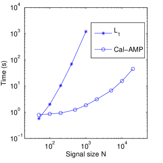
Figure 7: Left: Displacement of the phase transition with varying decalibration amplitude $w_{d}$. Parameters are $\rho=0.7$, $P=4$ and $N=10000$. While for very small decalibrations, the phase transition seems to be at the same location as in CS, it becomes clearly distinct with growing $w_{d}$. For each value of $w_{d}$, a vertical line materializes the empirical positions of the phase transitions (all points at the right of the line are perfectly reconstructed). Right: Running times of Cal-AMP compared to the $L_{1}$ minimizing algorithm used in [10]. Both algorithms ran on a 2.4GHz processor, parameters were $\rho=0.2$, $\alpha=1$, $P=5$. Note that using structured operators, as Fourier transforms, can significantly reduce running times [33].

Figure 8: Experimental phase diagrams for Cal-AMP and an $L_{1}$-minimizing algorithm using the CVX package [32], for $N=100$ and $w_{d}=0.1$. While both algorithms show a similar qualitative behavior, Cal-AMP requires significantly less measurements for successful reconstruction (white region). The line $\alpha_{\rm min}$ is a lower bound from (75), $\alpha^{\rm cal}$ is the phase transition of perfectly calibrated bayesian AMP, and $\alpha^{\rm cal}_{\rm DT}$ is the Donoho-Tanner phase transition of a perfectly calibrated $L_{1}$-based CS algorithm [34]. Just as the phase transition of Cal-AMP approaches $\alpha^{\rm cal}$ with growing $P$, the one of the $L_{1}$ algorithm approaches $\alpha^{\rm cal}_{\rm DT}$.

5.3 Complex gain calibration

For the numerical experiments, the distribution chosen for the calibration coefficients, the signal and the measurement matrix use the complex normal distribution with mean $R$ and variance $\Sigma$, which we note $\mathcal{CN}(x;R,\Sigma)$ :

$$p_{X}(x) =(1-\rho)\delta(x)+\rho\mathcal{CN}(x;0,1),$$ (87)

$$p_{F}(F) =\mathcal{CN}(F;0,1/N),$$ (88)

$$p_{D}(d) =\mathcal{CN}(d;0,10).$$ (89)

The corresponding Bayes-optimal update functions $\hat{f}^{X}$ and $\bar{f}^{X}$ have analytical expressions [33], given in appendix B. For the update functions $\hat{f}^{D}$ and $\bar{f}^{D}$, we use

$$\hat{f}^{D}(R,\Sigma) =\frac{R}{|R|}\frac{I(P+1,|R|,\Sigma,0,\infty)}{I(P,|R|,\Sigma,0,\infty)},$$ (90)

$$\bar{f}^{D}(R,\Sigma) =\Sigma.$$ (91)

Though not Bayes-optimal, they lead to good results, presented in Figure 9.

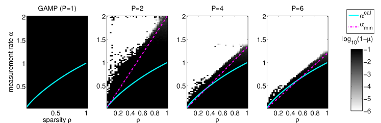
Figure 9: Experimental phase diagram for complex gain calibration using Cal-AMP for $N=500$. Here, $\alpha^{\rm cal}$ is the phase transition of a perfectly calibrated algorithm, that therefore performs as well as complex CS, analyzed in [33]. The line $\alpha_{\rm min}$ corresponds to the lower bound of (75).

6 Conclusion

In this paper, we have presented the Cal-AMP algorithm, designed for blind sensor calibration. Similar to GAMP, the framework allows to treat a variety of different problems beyond the case of compressed sensing. The derivation of the algorithm was detailed, starting from the probabilistic formulation of the problem and the message-passing algorithm derived from belief propagation. Two examples of problems falling into the Cal-AMP framework were studied numerically. Both for the faulty sensors problem and the gain calibration problem, the performance of Cal-AMP was found to be close to problem-specific lower bounds.

Cal-AMP could find concrete applications in experimental setups using physical devices for data acquisition, in which the ability to blindly calibrate the sensors might be either indispensable for good results, or allow substantial cuts in hardware costs.

In compressed sensing the asymptotic behavior of the AMP algorithm was analyzed via the state evolution equations [13, 15]. We attempted to derive the corresponding theory for Cal-AMP, but even on the heuristic level the corresponding generalization turns out to be non-trivial. This analysis is hence left as an interesting open problem.

Appendix A Approximation of $\psi$

We start by rewriting the messages (24) using the function $g_{0}$ introduced in (27):

$$\tilde{\psi}_{\mu l\to il}^{t+1}(x_{il}) \propto g_{0}(\mathbf{\hat{Z}}_{\mu l,i}^{t+1}+F_{\mu i}x_{il}\mathbf{e}_{1},\mathbf{\bar{Z}}_{\mu l,i}^{t+1},\mathbf{y}_{\mu}),$$ (92)

where $\mathbf{\hat{Z}}_{\mu l,i}^{t+1}$ is a $P$-dimensional vector with first component $\hat{Z}_{\mu l\to il}^{t+1}$, and its other components are $\hat{Z}_{\mu m}^{t}$ for $m\neq l$. The definition of $\mathbf{\bar{Z}}_{\mu l,i}^{t+1}$ is the same, replacing $\hat{Z}$ by $\bar{Z}$, and $\mathbf{y}_{\mu l}$ is the $P$-dimensional vector with first component $y_{\mu l}$ and other components $y_{\mu m}$ with $m\neq l$. Notice that due to the definition of $g_{0}$, the order of the components $2$ to $P$ of those vectors is unimportant as long as it is the same for each of them. $\mathbf{e}_{1}$ is the unit vector along the first direction of the $P$-dimensional space. Making a Taylor expansion of (92), we obtain

$$\tilde{\psi}_{\mu l\to il}^{t+1}(x_{il}) \propto{g_{0}(\mathbf{\hat{Z}}_{\mu l,i}^{t+1},\mathbf{\bar{Z}}_{\mu l,i}^{t+1},\mathbf{y}_{\mu})}$$ (93)

$$+x_{il}F_{\mu i}\frac{\partial g_{0}(\mathbf{\hat{Z}}_{\mu l,i}^{t+1},\mathbf{\bar{Z}}_{\mu l,i}^{t+1},\mathbf{y}_{\mu})}{\partial\hat{Z}_{\mu l\to il}^{t+1}}$$

$$+x_{il}^{2}\frac{F_{\mu i}^{2}}{2}\frac{\partial^{2}g_{0}(\mathbf{\hat{Z}}_{\mu l,i}^{t+1},\mathbf{\bar{Z}}_{\mu l,i}^{t+1},\mathbf{y}_{\mu})}{\partial(\hat{Z}_{\mu l\to il}^{t+1})^{2}}+x_{il}^{3}O(F_{\mu i}^{3}).$$

Let us now note that, for $a$ and $b$ of order one,

$$\mathcal{N}(x_{il};\frac{a}{F_{\mu i}b},-\frac{1}{F_{\mu i}^{2}b}) \propto\mathcal{N}(F_{\mu i}x_{il};\frac{a}{b},-\frac{1}{b})$$ (94)

$$\propto e^{F_{\mu i}x_{il}a+(F_{\mu i}x_{il})^{2}\frac{b}{2}}$$

$$\propto 1+F_{\mu i}x_{il}a+\frac{(F_{\mu i}x_{il})^{2}}{2}(b+a^{2})$$

$$+O(F_{\mu i}^{3}x_{il}^{3}).$$

We can now identify the coefficients of the expansion (93) with those in (94) to approximate the messages $\tilde{\psi}(x_{il})$ as Gaussians around $F_{\mu i}x_{il}=0$, with mean $\hat{p}$ and variance $\bar{p}$:

$$\tilde{\psi}_{\mu l\to il}^{t+1}(x_{il})\propto\mathcal{N}(x_{il};\hat{p}_{\mu l\to il},\bar{p}_{\mu l\to il})+O(F_{\mu i}^{3}x_{il}^{3}),$$ (95)

were $\hat{p}$ and $\bar{p}$ have following expressions, found by expressing the derivatives of $g_{0}$ with the functions $\hat{g}$ and $\bar{g}$ using the relations (28):

$$\bar{p}_{\mu l\to il} =(\bar{Z}_{\mu l\to il}^{t+1})^{2}\left(F_{\mu i}^{2}\left(\bar{Z}_{\mu l\to il}^{t+1}-\bar{z}_{\mu l\to il}^{t+1}\right)\right)^{-1},$$ (96)

$$\frac{\hat{p}_{\mu l\to il}}{\bar{p}_{\mu l\to il}} =\frac{F_{\mu i}}{\bar{Z}_{\mu l\to il}^{t+1}}\left(\hat{z}_{\mu l\to il}^{t+1}-\hat{Z}_{\mu l\to il}^{t+1}\right).$$ (97)

This expression (95) can now be used in (10):

$$\psi {}_{il\to\mu l}(x_{il})\propto p_{X}(x_{il})\prod_{\gamma\neq\mu}\tilde{\psi}_{\gamma l\to il}(x_{il})$$ (98)

$$\propto p_{X}(x_{il})\prod_{\gamma\neq\mu}\left(\mathcal{N}(x_{il};\hat{p}_{\gamma l\to il},\bar{p}_{\gamma l\to il})+O(F_{\gamma i}^{3}x_{il}^{3})\right)$$

$$\propto p_{X}(x_{il})\prod_{\gamma\neq\mu}\mathcal{N}(x_{il};\hat{p}_{\gamma l\to il},\bar{p}_{\gamma l\to il})\prod_{\gamma\neq\mu}\left(1+O(\frac{x_{il}^{3}}{N^{3/2}})\right)$$

The product of Gaussians that appears is proportional to another Gaussian. In fact,for any product of Gaussians,

$$\prod_{k=1}^{K}\mathcal{N}(x;R_{k},\Sigma_{k}) =\mathcal{N}(x;R,\Sigma)\frac{\prod_{k=1}^{K}\mathcal{N}(R_{k};0,\Sigma_{k})}{\mathcal{N}(R;0,\Sigma)},$$ (99)

with

$$\Sigma^{-1} =\sum_{k}\Sigma_{k}^{-1}\, R =\Sigma\sum_{k}\frac{R_{k}}{\Sigma_{k}}.$$ and (100)

Moreover, the logarithm of the second product is $\sum_{\gamma\neq\mu}x_{il}^{3}O(F_{\gamma i}^{3})=x_{il}^{3}O(1/\sqrt{N})$, so the product is $1+x_{il}^{3}O(1/\sqrt{N})$. The messages $\psi$ can therefore be written in the following way:

$$\psi_{\mu l\to il}^{t}({x}_{il})\propto p_{X}({x}_{il})\left(\mathcal{N}({x}_{il};\hat{X}_{il\to\mu l}^{t},\bar{X}_{il\to\mu l}^{t})+O(\frac{x_{il}^{3}}{\sqrt{N}})\right),$$

with

$$\bar{X}_{il\to\mu l}^{t+1} =\left(\sum_{\gamma\neq\mu}\frac{F_{\gamma i}^{2}\left(\bar{Z}_{\gamma l\to il}^{t+1}-\bar{z}_{\gamma l\to il}^{t+1}\right)}{(\bar{Z}_{\gamma l\to il}^{t+1})^{2}}\right)^{-1},$$

$$\hat{X}_{il\to\mu l}^{t+1} =\bar{X}_{il\to\mu l}^{t+1}\sum_{\gamma\neq\mu}\frac{F_{\gamma i}}{\bar{Z}_{\gamma l\to il}^{t+1}}\left(\hat{z}_{\gamma l\to il}^{t+1}-\hat{Z}_{\gamma l\to il}^{t+1}\right).$$

Appendix B Analytical expressions of update functions

B.1 Faulty sensors problem

$\hat{z}$ and $\bar{z}$ are obtained from the functions $\hat{g}$ and $\bar{g}$ such that:

$$\hat{z}_{\mu l} =\frac{\epsilon\hat{Z}_{\mu l}\pi^{f}_{\mu}+(1-\epsilon)y_{\mu l}\pi^{z}_{\mu}}{\epsilon\pi^{f}_{\mu}+(1-\epsilon)\pi^{z}_{\mu}},$$ (101)

$$\bar{z}_{\mu l} =\frac{\epsilon(\hat{Z}_{\mu l}^{2}+\bar{Z}_{\mu l})\pi^{f}_{\mu}+(1-\epsilon)|y_{\mu l}|^{2}\pi^{z}_{\mu}}{\epsilon\pi^{f}_{\mu}+(1-\epsilon)\pi^{z}_{\mu}}-|\hat{z}_{\mu l}|^{2},$$

with

$$\pi^{f}_{\mu} =\prod\limits_{m}\mathcal{N}(y_{\mu m};m_{f},\sigma_{f}^{2}),$$ (102)

$$\pi^{z}_{\mu} =\prod\limits_{m}\mathcal{N}(y_{\mu m};\hat{Z}_{\mu m},\bar{Z}_{\mu m}).$$ (103)

B.2 For Bernouilli-Gauss prior

the update functions $\hat{f}$ and $\bar{f}$ corresponding to the priors (76) and (87) can be found in [17] and [33] and obtained from:

$$f_{0}^{X}(\hat{X},\bar{X}) =(1-\rho)\mathcal{N}(\hat{X};0,\bar{X})+\rho\mathcal{N}(\hat{X};0,\bar{X}+1),$$

$$f_{1}^{X}(\hat{X},\bar{X}) =\rho\frac{\hat{X}}{\bar{X}+1}\mathcal{N}(\hat{X};0,\bar{X}+1),$$ (104)

$$f_{2}^{X}(\hat{X},\bar{X}) =\rho\frac{|\hat{X}|^{2}+\bar{X}(\bar{X}+1)}{(\bar{X}+1)^{2}}\mathcal{N}(\hat{X};0,\bar{X}+1).$$

In the complex case, all $\mathcal{N}$ are replaced by $\mathcal{CN}$.

References

• [1] E. Candès, J. Romberg, and T. Tao, “Robust uncertainty principles: Exact signal reconstruction from highly incomplete frequency information,” IEEE Trans. Inform. Theory, vol. 52, pp. 489–509, 2006.
• [2] M. Lustig, D. Donoho, and J. M. Pauly, “Sparse mri: The application of compressed sensing for rapid mr imaging,” Magnetic resonance in medicine, vol. 58, no. 6, pp. 1182–1195, 2007.
• [3] R. Otazo, D. Kim, L. Axel, and D. K. Sodickson, “Combination of compressed sensing and parallel imaging for highly accelerated first-pass cardiac perfusion mri,” Magnetic Resonance in Medicine, vol. 64, no. 3, pp. 767–776, 2010.
• [4] M. F. Duarte, M. A. Davenport, D. Takhar, J. N. Laska, T. Sun, K. F. Kelly, and R. G. Baraniuk, “Single-pixel imaging via compressive sampling,” Signal Processing Magazine, IEEE, vol. 25, no. 2, pp. 83–91, 2008.
• [5] S. Rangan, “Generalized approximate message passing for estimation with random linear mixing,” in Proc. of the IEEE Int. Symp. on Inform. Theory (ISIT), 2011, pp. 2168 –2172.
• [6] P. Schniter and S. Rangan, “Compressive phase retrieval via generalized approximate message passing,” in Communication, Control, and Computing (Allerton), 2012 50th Annual Allerton Conference on.   IEEE, 2012, pp. 815–822.
• [7] F. Krzakala, M. Mézard, and L. Zdeborová, “Phase diagram and approximate message passing for blind calibration and dictionary learning,” in Information Theory Proceedings (ISIT), 2013 IEEE International Symposium on.   IEEE, 2013, pp. 659–663.
• [8] U. Rau, S. Bhatnagar, M. A. Voronkov, and T. J. Cornwell, “Advances in calibration and imaging techniques in radio interferometry,” Proceedings of the IEEE, vol. 97, no. 8, 2009.
• [9] A. Levin, Y. Weiss, F. Durand, and W. T. Freeman, “Understanding and evaluating blind deconvolution algorithms,” in Computer Vision and Pattern Recognition, 2009. CVPR 2009. IEEE Conference on.   IEEE, 2009, pp. 1964–1971.
• [10] R. Gribonval, G. Chardon, and L. Daudet, “Blind calibration for compressed sensing by convex optimization,” in IEEE International Conference on Acoustics, Speech and Signal Processing (ICASSP), 2012, pp. 2713 – 2716.
• [11] H. Shen, M. Kleinsteuber, C. Bilen, and R. Gribonval, “A conjugate gradient algorithm for blind sensor calibration in sparse recovery,” in Machine Learning for Signal Processing (MLSP), 2013 IEEE International Workshop on.   IEEE, 2013, pp. 1–5.
• [12] C. Schulke, F. Caltagirone, F. Krzakala, and L. Zdeborová, “Blind calibration in compressed sensing using message passing algorithms,” in Advances in Neural Information Processing Systems, 2013, pp. 566–574.
• [13] D. L. Donoho, A. Maleki, and A. Montanari, “Message-passing algorithms for compressed sensing,” Proc. Natl. Acad. Sci., vol. 106, no. 45, pp. 18 914–18 919, 2009.
• [14] J. Yedidia, W. Freeman, and Y. Weiss, “Understanding belief propagation and its generalizations,” in Exploring Artificial Intelligence in the New Millennium.   San Francisco, CA, USA: Morgan Kaufmann, 2003, pp. 239–236.
• [15] M. Bayati and A. Montanari, “The dynamics of message passing on dense graphs, with applications to compressed sensing,” IEEE Transactions on Information Theory, vol. 57, no. 2, pp. 764 –785, 2011.
• [16] D. Donoho, A. Maleki, and A. Montanari, “Message passing algorithms for compressed sensing: I. motivation and construction,” in IEEE Information Theory Workshop (ITW), 2010, pp. 1 –5.
• [17] F. Krzakala, M. Mézard, F. Sausset, Y. Sun, and L. Zdeborová, “Probabilistic reconstruction in compressed sensing: Algorithms, phase diagrams, and threshold achieving matrices,” J. Stat. Mech., vol. P08009, 2012.
• [18] F. Caltagirone, L. Zdeborová, and F. Krzakala, “On convergence of approximate message passing,” in Information Theory (ISIT), 2014 IEEE International Symposium on.   IEEE, 2014, pp. 1812–1816.
• [19] S. Rangan, A. K. Fletcher, V. K. Goyal, and P. Schniter, “Hybrid generalized approximate message passing with applications to structured sparsity,” in Information Theory Proceedings (ISIT), 2012 IEEE International Symposium on.   IEEE, 2012, pp. 1236–1240.
• [20] M. Mézard and A. Montanari, Information, Physics, and Computation.   Oxford: Oxford Press, 2009.
• [21] U. S. Kamilov, A. Bourquard, E. Bostan, and M. Unser, “Autocalibrated signal reconstruction from linear measurements using adaptive gamp,” in Acoustics, Speech and Signal Processing (ICASSP), 2013 IEEE International Conference on.   Ieee, 2013, pp. 5925–5928.
• [22] P. Schniter, “A message-passing receiver for bicm-ofdm over unknown clustered-sparse channels,” Selected Topics in Signal Processing, IEEE Journal of, vol. 5, no. 8, pp. 1462–1474, 2011.
• [23] M. Nassar, P. Schniter, and B. L. Evans, “A factor graph approach to joint ofdm channel estimation and decoding in impulsive noise environments,” Signal Processing, IEEE Transactions on, vol. 62, no. 6, pp. 1576–1589, 2014.
• [24] D. J. Thouless, P. W. Anderson, and R. G. Palmer, “Solution of ‘solvable model of a spin-glass’,” Phil. Mag., vol. 35, pp. 593–601, 1977.
• [25] T. Heskes et al., “Stable fixed points of loopy belief propagation are minima of the bethe free energy,” Advances in neural information processing systems, vol. 15, pp. 359–366, 2003.
• [26] C. Lo, M. Liu, J. P. Lynch, and A. C. Gilbert, “Efficient sensor fault detection using combinatorial group testing,” in Distributed Computing in Sensor Systems (DCOSS), 2013 IEEE International Conference on.   IEEE, 2013, pp. 199–206.
• [27] A. Farruggia, G. Lo Re, and M. Ortolani, “Detecting faulty wireless sensor nodes through stochastic classification,” in Pervasive Computing and Communications Workshops (PERCOM Workshops), 2011 IEEE International Conference on.   IEEE, 2011, pp. 148–153.
• [28] J. Ziniel, P. Schniter, and P. Sederberg, “Binary linear classification and feature selection via generalized approximate message passing,” in Information Sciences and Systems (CISS), 2014 48th Annual Conference on.   IEEE, 2014, pp. 1–6.
• [29] S. Saleem and C. Vogel, “Adaptive blind background calibration of polynomial-represented frequency response mismatches in a two-channel time-interleaved adc,” Circuits and Systems I: Regular Papers, IEEE Transactions on, vol. 58, no. 6, pp. 1300–1310, 2011.
• [30] R. Gribonval, G. Chardon, and L. Daudet, “Blind calibration for compressed sensing by convex optimization,” in Acoustics, Speech and Signal Processing (ICASSP), 2012 IEEE International Conference on.   IEEE, 2012, pp. 2713–2716.
• [31] I. Corbella, A. Camps, F. Torres, and J. Bará, “Analysis of noise-injection networks for interferometric-radiometer calibration,” Microwave Theory and Techniques, IEEE Transactions on, vol. 48, no. 4, pp. 545–552, 2000.
• [32] M. Grant and S. Boyd, “CVX: Matlab software for disciplined convex programming, version 2.0 beta,” http://cvxr.com/cvx, 2012.
• [33] J. Barbier, F. Krzakala, and C. Schülke, “Compressed sensing and approximate message passing with spatially-coupled fourier and hadamard matrices,” arXiv preprint arXiv:1312.1740, 2013.
• [34] D. L. Donoho and J. Tanner, “Sparse nonnegative solution of underdetermined linear equations by linear programming,” Proc. Natl. Acad. Sci., vol. 102, no. 27, pp. 9446–9451, 2005.