A Diagrammer’s Note on Superconducting Fluctuation Transport for Beginners:
Supplement. Boltzmann Equation and Fermi-Liquid Theory

O. Narikiyo 111 Department of Physics, Kyushu University, Fukuoka 812-8581, Japan
( (April 1, 2021) )
Abstract

The effect of the collision term of the Boltzmann equation is discussed for the diagonal conductivity in the absence of magnetic field and the off-diagonal conductivity within the linear order of magnetic field. The consistency between the Boltzmann equation and the Fermi-liquid theory is confirmed. The electron-electron interaction is totally taken into account via the self-energy of the electron. The Umklappness is taken into account as the geometrical factor. The current-vertex correction in the fluctuation-exchange (FLEX) approximation violates these conventional schemes. In the Appendix the Tsuji formula, the geometrical formula for the Hall conductivity is discussed.

1 Introduction

This Note is the Supplement to arXiv:1112.1513 and arXiv:1203.0127. In the section 6 of the former and the footnote 4 of the latter, the exact treatment of the collision term of the Boltzmann equation (BE) is discussed and its consistency with the Fermi-liquid theory (FLT) is commented. In this Note the comment is expanded to be traceable. Especially it is stressed that the electron-electron interaction is totally taken into account via the self-energy of the electron. The Umklappness222 In this note I use the term $``$Umklappness” instead of $``$Umklapp scattering” to stress the fact that it is nothing but the ambiguity of the momentum-conservation modulo reciprocal lattice vectors. is taken into account as the geometrical factor. As a by-product it becomes clear how the fluctuation-exchange (FLEX) approximation violates these conventional schemes333 I have made other criticisms on the current-vertex correction in the FLEX approximation in arXiv:1204.5300 and arXiv:1301.5996. .

Although the other Notes in the series are written to be self-contained, this Note skips the calculations to obtain the results cited.

2 Collision Term

The linearized Boltzmann equation444 As discussed in the section 5 in arXiv:1112.1513 the temperature gradient is incorporated by the substitution $$e{\bf E}^{\prime}=e{\bf E}-\xi_{\bf p}{\nabla T\over T},$$ and the effect of the collision term can be analyzed in the same manner as in this Note. See Pikulin, Hou and Beenakker: Phys. Rev. B 84, 035133 (2011). in static and uniform electromagnetic field555 The complication arising from inhomogeneity or time-dependence of electromagnetic field is beyond the scope of the series of Notes. See, for example, Kita: Prog. Theor. Phys. 123, 581 (2010) for more general case. is

$$e{\bf E}\cdot{\bf v}_{\bf p}{\partial f(\xi_{\bf p})\over\partial\xi_{\bf p}}+e\big{(}{\bf v}_{\bf p}\times{\bf H}\big{)}\cdot{\partial g_{\bf p}\over\partial{\bf p}}=C_{\bf p}.$$ (1)

The collision term $C_{\bf p}$ is given as

$$C_{\bf p}=\sum_{\bf p^{\prime}}\Big{\{}C_{\bf pp^{\prime}}g_{\bf p^{\prime}}-C_{\bf p^{\prime}p}g_{\bf p}\Big{\}}\equiv-\sum_{\bf p^{\prime}}\big{(}\tau_{\rm tr}^{-1}\big{)}_{\bf pp^{\prime}}g_{\bf p^{\prime}},$$ (2)

with

$$\big{(}\tau_{\rm tr}^{-1}\big{)}_{\bf pp^{\prime}}={1\over\tau_{\bf p}}\delta_{\bf p,p^{\prime}}-C_{\bf pp^{\prime}},$$ (3)

and

$${1\over\tau_{\bf p}}\equiv\sum_{\bf p^{\prime}}C_{\bf p^{\prime}p}.$$ (4)

It is evident in (2) that the scattered-in term and the scattered-out term are the same interaction process666 If the scattering is restricted on the Fermi sphere, all the scattering events are treated on equal footing completely and the collision term for the component $g_{lm}$ of spherical harmonics $Y_{lm}$ becomes $$-{1\over\tau_{l}}g_{lm},$$ as (6.20) in [2]. This result strongly suggests that the effect of the interaction is essentially taken into account by the life-time and the other have only geometrical effects. but with different directions. More direct representation of this point is seen in the expression of the collision term in the quantum Boltzmann equation

$$\Sigma^{<}G^{>}-\Sigma^{>}G^{<},$$ (5)

as (8.293) in [3]. Namely, the effect of the interaction is totally expressed in terms of the self-energy $\Sigma$. The life-time $\tau_{\bf p}$ is determined by the imaginary part of the self-energy.

Thus the current-vertex correction in the FLEX approximation seems to be out of control. It violates the scheme of BE where the collision term is expressed in terms of the self-energy. It also violates the scheme of FLT, because FLT and BE give the same result for the conductivity tensor as discussed in the following. The correct current-vertex correction should be expressed in terms of the self-energy.

3 Diagonal Conductivity

The linearized Boltzmann equation is solved exactly [4] as discussed in the section 6 of arXiv:1112.1513 and the conductivity tensor per spin is expressed as

$$\sigma^{\mu\nu}=e^{2}\sum_{\bf p^{\prime}}\sum_{\bf p}v_{\bf p^{\prime}}^{\mu}A_{\bf p^{\prime}p}^{-1}v_{\bf p}^{\nu}\Big{(}-{\partial f(\xi_{\bf p})\over\partial\xi_{\bf p}}\Big{)},$$ (6)

with

$$A_{\bf pp^{\prime}}=\big{(}\tau_{\rm tr}^{-1}\big{)}_{\bf pp^{\prime}}-e\,\Big{(}{\bf v}_{\bf p}\times{\partial\over\partial{\bf p}}\Big{)}\cdot{\bf H}\,\,\delta_{\bf pp^{\prime}}.$$ (7)

The diagonal conductivity in the absence of magnetic field is obtained as

$$\sigma^{xx}=e^{2}\sum_{\bf p^{\prime}}\sum_{\bf p}v_{\bf p^{\prime}}^{x}\big{(}\tau_{\rm tr}\big{)}_{\bf p^{\prime}p}v_{\bf p}^{x}\Big{(}-{\partial f(\xi_{\bf p})\over\partial\xi_{\bf p}}\Big{)}.$$ (8)

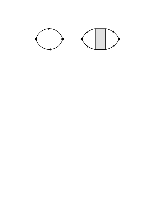
Diagrammatically (8) is expressed as Fig. 1. This result of BE is consistent with that of FLT with ${\bf k}=0$ and $\omega=0$ seen in (24) of [5] with (27) and in (4.38) of [6].


Refer to caption
Figure 1: The particle-hole pair in the left diagram, which represents the skeleton contribution to $\sigma^{xx}$, results in $\tau_{\bf p}$. The interaction between particle-hole pair in the right diagram represents the infinite repetition of $C_{\bf pp^{\prime}}$ and results in the renormalization of $\tau_{\bf p}$ into ${\tilde{\tau}}_{\bf p}$. Every dot at the ends of the diagrams represents $ev_{\bf p}^{x}$.

The expression (8) is not desirable, because it is not reduced into single-particle quantities. Such a reduction is the scheme of BE and can be accomplished easily in the isotropic case as

$$\sigma^{xx}=e^{2}\sum_{\bf p}v_{\bf p}^{x}{\tilde{\tau}}_{\bf p}v_{\bf p}^{x}\Big{(}-{\partial f(\xi_{\bf p})\over\partial\xi_{\bf p}}\Big{)},$$ (9)

where ${\tilde{\tau}}_{\bf p}$ is a scalar. This result777 Such a symmetry in $v_{\bf p}^{x}$ is obvious in the memory-function formalism [7]. of BE is consistent with that of FLT seen in (6.23) of [6] which takes into account the effect of Umklappness properly. Here the electron-electron interaction is totally taken into account via the self-energy of the electron; ${\bf v}_{\bf p}$ is renormalized888 Here the group velocity ${\bf v}_{\bf p}$ is determined by the renormalized band $\varepsilon({\bf p})$ of the quasi-particle as ${\bf v}_{\bf p}=\partial\varepsilon({\bf p})/\partial{\bf p}$. by the real part of the self-energy and ${\tilde{\tau}}_{\bf p}$ is determined999 We should evaluate an additional factor $C_{\bf p}$ resulted from the Umklappness so that ${\tilde{\tau}}_{\bf p}=\tau_{\bf p}/C_{\bf p}$ as seen in (6.23) of [6]. It should be noted that the effects of interaction and Umklappness are separable. The former determines the life-time $\tau_{\bf p}$ and the latter determines the factor $C_{\bf p}$ which reflects the momentum-conservation with additional reciprocal lattice vectors. by the imaginary part of the self-energy.

The symmetric form of (9) is expected from the vector character of the current vertex $v_{\bf p}^{x}$; the none-zero contribution after the ${\bf p}$-summation comes from the pair of observed current $e{\bf v}_{\bf p}$ and the current $e{\bf v}_{\bf p}$ coupled to the electric field with the same momentum. In other words the cause and the effect are in the same direction in isotropic systems101010 Even for anisotropic case, using the orthonormal vector set based on the Fermi-surface harmonics [8], it is concluded that $\sigma^{xx}$ is proportional to $(ev_{\bf p}^{x})^{2}$. . Perturbationally both currents should be $e{\bf v}_{\bf p}$ at the vertices of the observation and the coupling to the electric field. In terms of BE the electric current is given by $e{\bf v}_{\bf p}g_{\bf p}$ where the first order deviation of the distribution function $g_{\bf p}$ is proportional to the strength of the perturbation $e{\bf v}_{\bf p}\cdot{\bf A}$ where ${\bf E}=-\partial{\bf A}/\partial t$. In any way the contribution to the conductivity $\sigma^{xx}$ is proportional to $(ev_{\bf p}^{x})^{2}$.

Even in anisotropic cases111111 The symmetric form is obtained even for anisotropic cases; the conductivity is given as (1.4) in Okabe: J. Phys. Soc. Jpn. 68, 2721 (1999) where $l_{\bf p}^{x}$ is decomposed into ${\tilde{\tau}}_{\bf p}v_{\bf p}^{x}$ as the equation between (4.3) and (4.4) in Okabe: J. Phys. Soc. Jpn. 67, 4178 (1998). the reduction can be accomplished symmetrically with the help of the Fermi-surface harmonics [8]121212 On the basis of the Fermi-surface harmonics, all the elements in the theory are expressed as the polynomials of the velocity which is invariant under the transformation, ${\bf p}\rightarrow{\bf p}+{\bf K}$, with ${\bf K}$ being a reciprocal lattice vector. Thus it becomes clear that the Umklappness is nothing but the condition for the summation over ${\bf p}$. as seen in (2.1) of [9] which also takes into account the effect of Umklappness properly.

On the other hand, the asymmetric expression131313 By introducing the expansion of $J_{\bf p}^{x}$ in terms of the Fermi-surface harmonics, it is shown that all the terms orthogonal to $v_{\bf p}^{x}$ do not contribute to $\sigma^{xx}$ in Maebashi and Fukuyama: J. Phys. Soc. Jpn. 66, 3577 (1997).

$$\sigma^{xx}=e^{2}\sum_{\bf p}v_{\bf p}^{x}{1\over 2\gamma_{\bf p}}J_{\bf p}^{x}\Big{(}-{\partial f(\xi_{\bf p})\over\partial\xi_{\bf p}}\Big{)},$$ (10)

seen in (1.2) of [10] is misleading; it gives a wrong impression that there might be something in the current-vertex correction renormalizing $v_{\bf p}^{x}$ into $J_{\bf p}^{x}$. I suspect that the current-vertex correction in the FLEX approximation [11] is driven by such a wrong impression. Although the vertex correction should be in harmony with the imaginary part of the single-particle self-energy, that in the FLEX approximation is out of control.

4 Off-diagonal Conductivity

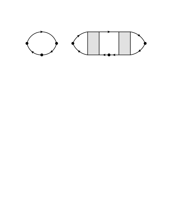
Combined with the discussion leading to (9), the solution of BE for $\sigma^{xy}$ in the section 6 of arXiv:1112.1513 is reduced into

$$\sigma^{xy}=e^{3}\sum_{\bf p}v_{\bf p}^{x}{\tilde{\tau}}_{\bf p}\,\Big{(}{\bf v}_{\bf p}\times{\partial\over\partial{\bf p}}\Big{)}\cdot{\bf H}\,\,{\tilde{\tau}}_{\bf p}v_{\bf p}^{y}\,\Big{(}-{\partial f(\xi_{\bf p})\over\partial\xi_{\bf p}}\Big{)},$$ (11)

within the linear order of magnetic field. Diagrammatically (11) is expressed as Fig. 2. This result of BE is consistent with that of FLT141414 Since the current-vertex correction there is not reduced into the single-particle quantities, (1.7) in [10] is misleading as discussed in the previous section. seen in (35) of [12]151515 An important point stressed in this reference is the absence of the interaction renormalization in the Hall coefficient. . Within the linear response the collision term is evaluated in the absence of the external electromagnetic fields so that there is no new interaction effect by the introduction of the magnetic field. Namely, the introduction of the magnetic field is not a many-body problem but a single-body problem161616 The effect of the Lorentz force on the single-body state is the problem. as discussed in the next section.


Refer to caption
Figure 2: Here I show only two typical diagrams which contribute to $\sigma^{xy}$. The skeleton process in the left diagram results in $(\tau_{\bf p})^{2}$. The right diagram contains the skeleton structure at its center and the interactions at both ends result in the renormalization of $(\tau_{\bf p})^{2}$ into $({\tilde{\tau}}_{\bf p})^{2}$. Only the most divergent contribution in terms of $1/\tau_{\bf p}$ is taken into account in FLT and the skeleton structure is necessary for such a contribution. In each diagram the left-end and right-end dots represent $ev_{\bf p}^{x}$ and $ev_{\bf p}^{y}$ respectively and the center dot represents the coupling $e{\bf v}_{\bf p}\cdot{\bf A}$ where ${\bf H}=i({\bf k}\times{\bf A})$.

This expression (11) is unsatisfactory by the following two reasons. (i) The Onsager relation, $\sigma^{yx}=-\sigma^{xy}$, is not evident. (See arXiv:2011.04421 for details.) (ii) The derivative of ${\tilde{\tau}}_{\bf p}$ is not found in the diagrammatic analysis. These are resolved as follows.

I anti-symmetrize $\sigma^{xy}$ by force171717 The same procedure is necessary to obtain a beautiful geometric formula of ${\hat{\sigma}}^{xy}$ in Ong: Phys. Rev. B 43, 193 (1991) where the element of the line-integral ${\rm d}l_{x}l_{y}$ obtained from $\sigma^{xy}$ is anti-symmetrized into $({\rm d}{\vec{l}}\times{\vec{l}})_{z}$. into ${\hat{\sigma}}^{xy}\equiv(\sigma^{xy}-\sigma^{yx})/2$ where

$$\sigma^{yx}=e^{3}\sum_{\bf p}v_{\bf p}^{y}{\tilde{\tau}}_{\bf p}\,\Big{(}{\bf v}_{\bf p}\times{\partial\over\partial{\bf p}}\Big{)}\cdot{\bf H}\,\,{\tilde{\tau}}_{\bf p}v_{\bf p}^{x}\,\Big{(}-{\partial f(\xi_{\bf p})\over\partial\xi_{\bf p}}\Big{)}.$$ (12)

If ${\bf H}=(0,0,H)$, we obtain

$${\hat{\sigma}}^{xy}=-{\hat{\sigma}}^{yx}={e^{3}H\over 2}\sum_{\bf p}{\tilde{\tau}}_{\bf p}^{2}\,h({\bf v}_{\bf p},{\partial\over\partial{\bf p}})\,\Big{(}-{\partial f(\xi_{\bf p})\over\partial\xi_{\bf p}}\Big{)},$$ (13)

with

$$h({\bf v}_{\bf p},{\partial\over\partial{\bf p}})\equiv(v^{x}_{\bf p})^{2}{\partial v^{y}_{\bf p}\over\partial p^{y}}-v^{x}_{\bf p}v^{y}_{\bf p}{\partial v^{y}_{\bf p}\over\partial p^{x}}-v^{y}_{\bf p}v^{x}_{\bf p}{\partial v^{x}_{\bf p}\over\partial p^{y}}+(v^{y}_{\bf p})^{2}{\partial v^{x}_{\bf p}\over\partial p^{x}}.$$ (14)

This result of BE is consistent with the general result of FLT seen in (3.21) of [10]. (13) reduces to (11) when $x$- and $y$- directions are equivalent as discussed in [10].

It should be noted that the derivatives of ${\tilde{\tau}}_{\bf p}$ cancel out through this anti-symmetrization.

5 Coupling to Magnetic Field

The introduction of the magnetic field is discussed by various means. I will comment on three kinds of means in the following. All lead to the consistent result with BE181818 In the derivation of BE via the Wigner function $$f_{\rm W}({\bf p},{\bf R},t)=\int{\rm d}{\bf r}\exp\big{[}-i{\bf r}\cdot\big{(}{\bf p}-e{\bf A}({\bf R},t)\big{)}\big{]}\Big{\langle}{\bf R}+{{\bf r}\over 2}\Big{|}{\hat{\rho}}(t)\Big{|}{\bf R}-{{\bf r}\over 2}\Big{\rangle},$$ the Lorentz force appears as seen in (4.78) of [13]. . It should be noted that the introduction of the magnetic field is a single-body problem.

(A) Vector Potential

If we set ${\bf A}({\bf x})=\exp(i{\bf k}\cdot{\bf x})$ with a constant vector ${\bf A}$, the magnetic field ${\bf H}$ is given by

$${\bf H}=i({\bf k}\times{\bf A}),$$ (15)

in the limit of ${\bf k}\rightarrow 0$. For anisotropic systems the extraction of this factor from Feynman diagrams with full interaction is rather complicated task191919 This task can be circumvented by use of the Ward identity as discussed in Itoh: J. Phys. F 14, L89 (1984). as done in [10, 14]. However, it is sufficient to show the means in the case of the relaxation-time approximation, because the interaction effect beyond this approximation only leads to the renormalization of $\tau_{\bf p}$ as has been discussed in the previous section. This task202020 For the extraction of the factor, $(k^{x}A^{y}-k^{y}A^{x})$, see Fig. 1 of arXiv:1203.0127. The processes (a) and (b) lead to the contribution proportional to $$v^{x}_{\bf p}\big{(}v^{x}_{\bf p}A^{x}+v^{y}_{\bf p}A^{y}\big{)}\big{(}{\partial v^{y}_{\bf p}\over\partial p^{x}}k^{x}+{\partial v^{y}_{\bf p}\over\partial p^{y}}k^{y}\big{)},$$ where ${\bf A}$-linear term comes from the propagator and ${\bf k}$-linear term comes from the current, and the process (c) leads to $$-v^{x}_{\bf p}\big{(}v^{x}_{\bf p}k^{x}+v^{y}_{\bf p}k^{y}\big{)}\big{(}{\partial v^{y}_{\bf p}\over\partial p^{x}}A^{x}+{\partial v^{y}_{\bf p}\over\partial p^{y}}A^{y}\big{)},$$ where ${\bf k}$-linear term comes from the propagator and ${\bf A}$-linear term comes from the current, for general anisotropic case when ${\bf A}=(A^{x},A^{y},0)$ and ${\bf k}=(k^{x},k^{y},0)$. These results are obtained by the same manner as in the isotropic case, arXiv:1203.0127, only by generalizing the electric current (8) there to $$j_{\mu}^{H}(0)=e\sum_{\sigma}\sum_{\bf p}{\partial\varepsilon({\bf p}-e{\bf A})\over\partial p^{\mu}}c_{{\bf p}\sigma}^{\dagger}c_{{\bf p}\sigma},$$ and lead to (18) in the next footnote times the magnetic field $H=i(k^{x}A^{y}-k^{y}A^{x})$ where ${\bf H}=(0,0,H)$. Here the ${\bf k}$-linear expansion of $v_{\bf p}^{y}$ in (a) and (b) is generalized as $${1\over m}k^{y}\rightarrow{\partial^{2}\varepsilon({\bf p})\over\partial p^{x}\partial p^{y}}k^{x}+{\partial^{2}\varepsilon({\bf p})\over\partial p^{y}\partial p^{y}}k^{y},$$ where $\partial\varepsilon({\bf p})/\partial{\bf p}={\bf v}_{\bf p}$. The ${\bf A}$-linear expansion in (c) is generalized as $${1\over m}A^{y}\rightarrow{\partial^{2}\varepsilon({\bf p})\over\partial p^{x}\partial p^{y}}A^{x}+{\partial^{2}\varepsilon({\bf p})\over\partial p^{y}\partial p^{y}}A^{y}.$$ is a straightforward one.

(B) Magnetic Flux

The effect of the magnetic field appears as the phase factor of the electron propagator as

$$G({\bf r}_{1},{\bf r}_{2})=\exp\big{[}ie\Phi({\bf r}_{1},{\bf r}_{2})\big{]}G({\bf r}_{1}-{\bf r}_{2}).$$ (16)

Namely, the interaction affects only translationally invariant propagator $G({\bf r}_{1}-{\bf r}_{2})$ and the phase $\Phi({\bf r}_{1},{\bf r}_{2})$ is determined geometrically. These two are separable and the propagator in the presence of the magnetic field $G({\bf r}_{1},{\bf r}_{2})$ is the product of these. The calculation of the loop diagram which corresponds to the conductivity leads to the magnetic flux as discussed in [12, 15].

(C) Cyclotron Motion

The magnetic field enters into the equation of motion as the cyclotron frequency as

$${\dot{J}}_{y}={1\over i}\big{[}J_{y},K\big{]}=\omega_{c}J_{x},$$ (17)

for isotropic case212121 Even for anisotropic case the equation of motion for the center-of-mass current is easily calculated as $${\dot{J}}_{y}=eH\big{(}m^{-1}_{yx}J_{y}-m^{-1}_{yy}J_{x}\big{)}.$$ Classically the Lorentz force $${\hat{m}}{\dot{\bf v}}=e({\bf v}\times{\bf H}),$$ leads to $$\left(\begin{array}[]{c}{\dot{v}}_{x}\\ {\dot{v}}_{y}\\ \end{array}\right)=eH\left(\begin{array}[]{cc}m^{-1}_{xx}&m^{-1}_{xy}\\ m^{-1}_{yx}&m^{-1}_{yy}\\ \end{array}\right)\left(\begin{array}[]{c}v_{y}\\ -v_{x}\\ \end{array}\right),$$ when ${\bf H}=(0,0,H)$. Since $\sigma^{xy}$ is proportional to the expectation value of $v_{x}{\dot{v}}_{y}$, we obtain the factor $$v_{x}\big{(}m^{-1}_{yy}v_{x}-m^{-1}_{yx}v_{y}\big{)},$$ as seen in (12.5.9) of Ziman: Electrons and Phonons (Clarendon, Oxford, 1960). The general expression of this factor becomes $$v^{x}_{\bf p}\Big{(}v^{x}_{\bf p}{\partial\over\partial p^{y}}-v^{y}_{\bf p}{\partial\over\partial p^{x}}\Big{)}v^{y}_{\bf p}={\partial\varepsilon({\bf p})\over\partial p^{x}}\Big{(}{\partial\varepsilon({\bf p})\over\partial p^{x}}{\partial^{2}\varepsilon({\bf p})\over\partial p^{y}\partial p^{y}}-{\partial\varepsilon({\bf p})\over\partial p^{y}}{\partial^{2}\varepsilon({\bf p})\over\partial p^{x}\partial p^{y}}\Big{)}.$$ (18) where ${\bf J}$ is the center-of-mass current222222 The equation of motion for the center-of-mass current is independent of the interaction so that the factor $v_{x}(m^{-1}_{yy}v_{x}-m^{-1}_{yx}v_{y})$ is independent of the interaction. Such a conclusion is a corollary of Kohn’s theorem: Phys. Rev. 123, 1242 (1961). . The calculation of the memory function232323 The scalar memory function is insufficient to construct a consistent transport theory. We have to use the matrix memory function as discussed in [7, 9]. leads to the consistent result [16, 17] with (11).

6 Remarks

Finally it is stressed that the effect of the electron-electron interaction on the conductivity tensor is totally taken into account via the self-energy of the electron. It is completely embodied in the conventional schemes of BE and FLT where the Umklappness and the anisotropy of the Fermi surface are properly taken into account.

The sections of Exercise and Acknowledgements are common to those in arXiv:1112.1513 so that I do not repeat here. Eq. (76) in arXiv:1112.1513 should be

$$\left(\begin{array}[]{c}{\bf J}^{e}\\ {\bf J}^{Q}\\ \end{array}\right)=\left(\begin{array}[]{cc}\sigma&\alpha\\ \tilde{\alpha}&\kappa\\ \end{array}\right)\left(\begin{array}[]{c}{\bf E}\\ -\nabla T\\ \end{array}\right).$$

7 Appendix

In this Appendix242424 This Appendix is the reproduction of http://hdl.handle.net/2324/2344834. the Tsuji formula for the Hall conductivity in metals is discussed in Haldane’s framework. (See arXiv:2011.04421 for details.)

The Tsuji formula [Tsuji] is widely known as a geometrical formula for the Hall conductivity in metals under weak magnetic field. Since it was derived under the assumption of the cubic symmetry, Haldane [Haldane] tried to eliminate the assumption. Here we discuss the Tsuji formula using Haldane’s framework. However, our conclusion is different from Haldane’s. The details252525 This Appendix is a nutshell of our previous note, http://hdl.handle.net/2324/1957531. are described in http://hdl.handle.net/2324/1957531.

In usual notation the weak-field DC Hall conductivity tensor $\sigma^{xy}$ per spin is given by [Tsuji, Haldane]

$$\sigma^{xy}=e^{3}B\int{{\rm d}S\over(2\pi)^{3}}\left(v^{x}\!,\,v^{y}\right)\begin{pmatrix}M^{-1}_{yy}&-M^{-1}_{yx}\\ 0&0\end{pmatrix}\begin{pmatrix}v^{x}\\ v^{y}\end{pmatrix}{\tau^{2}\over|{\vec{v}}|},$$ (19)

for the Fermi surface contribution in metals. Throughout this note we only consider the contribution from a single sheet of the Fermi surface. Here the magnetic field is chosen as ${\vec{B}}=(0,0,B)$. The quasi-particle velocity ${\vec{v}}=(v^{x},v^{y},v^{z})$ and the effective mass tensor $M_{\alpha\beta}$ are given by the derivative of the quasi-particle energy $\varepsilon$: $v^{\alpha}=\partial\varepsilon/\partial k^{\alpha}$ and $M_{\alpha\beta}^{-1}=\partial^{2}\varepsilon/\partial k^{\alpha}\partial k^{\beta}$. Since the contribution of the derivative of $\tau$ does not appear in the antisymmetric tensor $(\sigma^{xy}-\sigma^{yx})/2$, we have dropped it.

Experimentally $\sigma^{xy}$ is obtained from the measurement where we measure the current in $x$-direction under the electric field in $y$-direction and the magnetic field in $z$-direction. If we measure the current in $y$-direction under the electric field in $x$-direction and the magnetic field in $z$-direction, we obtain $\sigma^{yx}$ described as

$$-\sigma^{yx}=e^{3}B\int{{\rm d}S\over(2\pi)^{3}}\left(v^{x}\!,\,v^{y}\right)\begin{pmatrix}0&0\\ -M^{-1}_{xy}&M^{-1}_{xx}\end{pmatrix}\begin{pmatrix}v^{x}\\ v^{y}\end{pmatrix}{\tau^{2}\over|{\vec{v}}|}.$$ (20)

Haldane [Haldane] introduced the symmetric tensor $e^{3}B\gamma_{zz}\equiv(\sigma^{xy}-\sigma^{yx})/2$. Eq. (19) and Eq. (20) lead to

$$\gamma_{zz}={1\over 2}\int{{\rm d}S\over(2\pi)^{3}}\left(v^{x}\!,\,v^{y}\right)\begin{pmatrix}M^{-1}_{yy}&-M^{-1}_{yx}\\ -M^{-1}_{xy}&M^{-1}_{xx}\end{pmatrix}\begin{pmatrix}v^{x}\\ v^{y}\end{pmatrix}{\tau^{2}\over|{\vec{v}}|}.$$ (21)

Other symmetric tensors are introduced in the same manner as $e^{3}B\gamma_{xx}\equiv(\sigma^{yz}-\sigma^{zy})/2$ and $e^{3}B\gamma_{yy}\equiv(\sigma^{zx}-\sigma^{xz})/2$. As shown in the following the geometrical nature is captured by these symmetric tensors. It should be noted that our result, Eq. (21), is different form Haldane’s [Haldane]. The difference arises from the following fact. While Eq. (21) contains $(\partial v^{x}/\partial k^{y})/|{\vec{v}}|$, Haldane erroneously uses $\partial(v^{x}/|{\vec{v}}|)/\partial k^{y}$ instead.

The target of our geometrical description is the mean curvature $H$ of the Fermi surface. It is given by

$\displaystyle 2H$ $\displaystyle=$ $\displaystyle{1\over|{\vec{v}}|^{3}}\cdot\Big{[}\varepsilon_{x}\varepsilon_{x}(\varepsilon_{yy}+\varepsilon_{zz})+\varepsilon_{y}\varepsilon_{y}(\varepsilon_{zz}+\varepsilon_{xx})+\varepsilon_{z}\varepsilon_{z}(\varepsilon_{xx}+\varepsilon_{yy})$
$\displaystyle-$ $\displaystyle\varepsilon_{x}(\varepsilon_{y}\varepsilon_{yx}+\varepsilon_{z}\varepsilon_{zx})-\varepsilon_{y}(\varepsilon_{x}\varepsilon_{xy}+\varepsilon_{z}\varepsilon_{zy})-\varepsilon_{z}(\varepsilon_{x}\varepsilon_{xz}+\varepsilon_{y}\varepsilon_{yz})\Big{]},$

for any shape of the Fermi surface. Here we have used the notations $\varepsilon_{\alpha}\equiv v^{\alpha}$ and $\varepsilon_{\alpha\beta}\equiv M_{\alpha\beta}^{-1}$.

The geometrical information in our master equation, Eq. (21), is represented by $h_{zz}$ as

$$\gamma_{zz}=\int{{\rm d}S\over(2\pi)^{3}}h_{zz}\tau^{2},$$

with

$$h_{zz}={1\over 2|{\vec{v}}|}\left(\varepsilon_{x}\varepsilon_{x}\varepsilon_{yy}+\varepsilon_{y}\varepsilon_{y}\varepsilon_{xx}-\varepsilon_{x}\varepsilon_{y}\varepsilon_{yx}-\varepsilon_{y}\varepsilon_{x}\varepsilon_{xy}\right).$$

Using

$$h_{xx}={1\over 2|{\vec{v}}|}\left(\varepsilon_{y}\varepsilon_{y}\varepsilon_{zz}+\varepsilon_{z}\varepsilon_{z}\varepsilon_{yy}-\varepsilon_{y}\varepsilon_{z}\varepsilon_{zy}-\varepsilon_{z}\varepsilon_{y}\varepsilon_{yz}\right),$$

and

$$h_{yy}={1\over 2|{\vec{v}}|}\left(\varepsilon_{z}\varepsilon_{z}\varepsilon_{xx}+\varepsilon_{x}\varepsilon_{x}\varepsilon_{zz}-\varepsilon_{z}\varepsilon_{x}\varepsilon_{xz}-\varepsilon_{x}\varepsilon_{z}\varepsilon_{zx}\right),$$

additionally, we obtain

$$\gamma_{zz}+\gamma_{xx}+\gamma_{yy}=\int{{\rm d}S\over(2\pi)^{3}}Hl^{2},$$ (22)

with $l^{2}=|{\vec{v}}|^{2}\tau^{2}$. Our result, Eq. (22), is applicable to any shape of the Fermi surface. In the case of cubic symmetry Eq. (22) is reduced to the Tsuji formula [Tsuji, Haldane]

$\displaystyle\gamma_{zz}=\gamma_{xx}=\gamma_{yy}=\int{{\rm d}S\over(2\pi)^{3}}{H\over 3}l^{2}.$

Experimentally $\gamma_{cc}$ is obtained from the measurements of $\sigma^{ab}$ and $\sigma^{ba}$ where $(c,a,b)=(z,x,y),(x,y,z),(y,z,x)$. By summing six experimental results with different configurations we can use Eq. (22).


[Tsuji] Tsuji: J. Phys. Soc. Jpn. 13, 979 (1958).

[Haldane] Haldane: arXiv:cond-mat/0504227v2.

References

  • [1] As mentioned in the Introduction, this Note skips the calculations to obtain the results cited. Thus the character of the following references is different from those of the other Notes in this series. I only list the references convenient for my explanation. Neither originality nor priority is considered here.
  • [2] Peierls: Quantum Theory of Solids (Clarendon, Oxford, 1955).
  • [3] Mahan: Many-Particle Physics 3rd (Kluwer/Plenum, New York, 2000).
  • [4] Kotliar, Sengupta and Varma: Phys. Rev. B 53, 3573 (1996).
  • [5] Éliashberg: Sov. Phys. JETP 14, 886 (1962).
  • [6] Yamada and Yosida: Prog. Theor. Phys. 76, 621 (1986).
  • [7] Hartnoll and Hofman: Phys. Rev. Lett. 108, 241601 (2012).
  • [8] Allen: Phys. Rev. B 13, 1416 (1976).
  • [9] Maebashi and Fukuyama: J. Phys. Soc. Jpn. 67, 242 (1998).
  • [10] Kohno and Yamada: Prog. Theor. Phys. 80, 623 (1988).
  • [11] Kontani: Pep. Prog. Phys. 71, 026501 (2008).
  • [12] Khodas and Finkel’stein: Phys. Rev. B 68, 155114 (2003).
  • [13] Rammer: Quantum Transport Theory (Perseus Books, Reading Massachusetts, 1998).
  • [14] Fukuyama, Ebisawa and Wada: Prog. Theor. Phys. 42, 494 (1969).
  • [15] Edelstein: JETP Lett. 67, 159 (1998).
  • [16] Ting, Ying and Quinn: Phys. Rev. B 16, 5394 (1977).
  • [17] Shiwa and Ishihara: J. Phys. C 16, 4853 (1983).