Kinetic Reverse $k$-Nearest Neighbor Problem 

Abstract

This paper provides the first solution to the kinetic reverse $k$-nearest neighbor (R$k$NN) problem in $\mathbb{R}^{d}$, which is defined as follows: Given a set $P$ of $n$ moving points in arbitrary but fixed dimension $d$, an integer $k$, and a query point $q\notin P$ at any time $t$, report all the points $p\in P$ for which $q$ is one of the $k$-nearest neighbors of $p$.

1 Introduction

The reverse $k$-nearest neighbor (R$k$NN) problem is a popular variant of the $k$-nearest neighbor ($k$NN) problem and asks for the influence of a query point on a point set. Unlike the $k$NN problem, the exact number of reverse $k$-nearest neighbors of a query point is not known in advancem, but as we prove in this paper the number is upper-bounded by $O(k)$. The R$k$NN problem is formally defined as follows: Given a set $P$ of $n$ points in $\mathbb{R}^{d}$, an integer $k$, $1\leq k\leq n-1$, and a query point $q\notin P$, find the set $\mbox{R$k$NN}(q)$ of all $p$ in $P$ for which $q$ is one of $k$-nearest neighbors of $p$. Thus $\mbox{R$k$NN}(q)=\{p\in P:~{}|pq|\leq|pp_{k}|\}$, where $|.|$ denotes Euclidean distance, and $p_{k}$ is the $k^{th}$ nearest neighbor of $p$ among the points in $P$. The kinetic R$k$NN problem is to answer R$k$NN queries on a set $P$ of moving points, where the trajectory of each point $p\in P$ is a function of time. Here, we assume the trajectories are polynomial functions of maximum degree bounded by some constant $s$.

Related work.

The reverse $k$-nearest neighbor problem was first posed by Korn and Muthukrishnan [13] in the database community, and then considered extensively in this community due to its many applications, e.g., decision support systems, profile-based marketing, traffic networks, business location planning, clustering and outlier detection, and molecular biology. The reverse $k$-nearest neighbor queries for a set of continuously moving objects has also attracted the attention of the database community; see [8] and references therein. Examples of moving objects include players in multi-player game environments, soldiers in a battlefield, tourists in dangerous environments, and mobile devices in wireless ad-hoc networks.

To our knowledge, in computational geometry, there exist two data structures [14, 9] that give solutions to the R$k$NN problem. Both of these solutions answer R$k$NN queries for a set $P$ of stationary points and both only work for $k=1$. Maheshwari et al. (2002) [14] gave a data structure to solve the R$1$NN problem in $\mathbb{R}^{2}$. Their data structure creates an arrangement of largest empty circles centered at the points of $P$ and answers R$1$NN queries by point location in the arrangement. Their data structure uses $O(n)$ space and $O(n\log n)$ preprocessing time, and an R$1$NN query can be answered in time $O(\log n)$. Cheong et al. (2011) [9] considered the R$1$NN problem in $\mathbb{R}^{d}$, where $d=O(1)$. Their method, which uses a compressed quadtree, partitions space into cells such that each cell contains a small number of candidate points. To answer an R$1$NN query, their solution finds a cell that contains the query point and then checks all the points in the cell. Their approach uses $O(n)$ space and $O(n\log n)$ preprocessing time, and can answer an R$1$NN query in $O(\log n)$ time. It seems that the approach by Cheong et al. can be extended to answer R$k$NN queries with preprocessing time $O(kn\log n)$, space $O(kn)$, and query time $O(\log n+k)$.

For a set $P$ of $n$ stationary points, one can report all the $1$-nearest neighbors in time $O(n\log n)$ [18], and all the $k$-nearest neighbors, for any $k\geq 1$, in time $O(kn\log n)$ [12], where the neighbors are reported in order of increasing distance from each point; reporting the unordered set takes time $O(n\log n+kn)$ [5, 10, 12].

For a set of moving points, there are three kinetic data structures (KDS’s) [2, 16, 17] to maintain all the $k$-nearest neighbors, but they only work for $k=1$.

Our contribution.

For a set $P$ of $n$ continuously moving points in $\mathbb{R}^{d}$, where the trajectory of each point is a polynomial function of at most constant degree $s$, we provide a simple kinetic approach to answer R$k$NN queries on the moving points. In fact, we provide the first solution to the kinetic R$k$NN problem for any $k\geq 1$ in any fixed dimension $d$. To answer an R$k$NN query for a query point $q\notin P$ at any time $t$, we partition the $d$-dimensional space into a constant number of cones around $q$, and then among the points of $P$ in each cone, we examine the $k$ points having shortest projections on the cone axis. We obtain $O(k)$ candidate points for $q$ such that $q$ might be one of their $k$-nearest neighbors at time $t$. To check which if any of these candidate points is a reverse $k$-nearest neighbor of $q$, we maintain the $k^{th}$ nearest neighbor $p_{k}$ of each point $p\in P$ over time. By checking whether $|pq|\leq|pp_{k}|$ we can easily check whether a candidate point $p$ is one of the reverse $k$-nearest neighbors of $q$ at time $t$.

In the preprocessing step, we introduce a method for reporting all the $k$-nearest neighbors for all the points $p\in P$ in order of increasing distance from $p$. For $k=\Omega(\log^{d-1}n)$, both our method and the method of Dickerson and Eppstein [12] give the same complexity, but in our view, our method is simpler in practice.

In order to answer R$k$NN queries, our kinetic approach maintains all the $k$-nearest neighbors over time. This is the first KDS for maintenance of all the $k$-nearest neighbors in $\mathbb{R}^{d}$, for any $k\geq 1$. Our KDS uses $O(n\log^{d+1}n+kn)$ space and $O(n\log^{d+1}n+kn\log n)$ preprocessing time, and processes $O(\phi(s,n)*n^{2})$ events, each in amortized time $O(\log n)$. Here, $\phi(s,n)$ is the complexity of the $k$-level of a set of $n$ partially-defined polynomial functions, such that each pair of them intersects at most $s$ times. The current bounds on $\phi(s,n)$ are as follows [6, 7].

$$\phi(s,n)=\begin{cases}{O(n^{3/2}\log n)},&\text{for $s=2$};\\ {O(n^{5/3}\text{poly}\log n)},&\text{for $s=3$};\\ {O(n^{31/18}\text{poly}\log n)},&\text{for $s=4$};\\ {O(n^{161/90-\delta})},&\text{for $s=5$, for some constant $\delta>0$};\\ {O(n^{2-1/2s-\delta_{s}})},&\text{for odd $s$, for some constant $\delta_{s}>0$};\\ {O(n^{2-1/2(s-1)-\delta_{s}})},&\text{for even $s$, for some constant $\delta_{s}>0$}.\end{cases}$$

At any time $t$, an R$k$NN query can be answered in time $O(\log^{d}n+k)$. Note that if an event occurs at the same time $t$, we first spend amortized time $O(\log n)$ to update all the $k$-nearest neighbors, and then we answer the query.

Outline.

Section 2 provides two key lemmas, and in fact introduces a new supergraph, namely the $k$-Semi-Yao graph, of the $k$-nearest neighbor graph. In Section 3, we show how to report all the $k$-nearest neighbors. Section 4 gives a (kinetic) data structure for answering R$k$NN queries on moving points, where the trajectory of each point is a bounded-degree polynomial. Section 5 concludes.

2 Key Lemmas

Partition the plane around the origin $o$ into six wedges, $W_{0},...,W_{5}$, each of angle $\pi/3$ (see Figure 1(a)). Denote by $W_{l}(p)$ the translation of wedge $W_{l}$, $0\leq l\leq 5$, such that its apex moves from $o$ to point $p$ (see Figure 1(b)). Denote by $x_{l}$ (resp. $x_{l}(p)$) the vector along the bisector of $W_{l}$ (resp. $W_{l}(p)$) directed outward from the apex at $o$ (resp. $p$). Denote the reflection of $W_{l}(p)$ through $p$ by $W_{l^{\prime}}(p)$. Note that $l^{\prime}=(l+3)\bmod{6}$; see Figure 1(b).

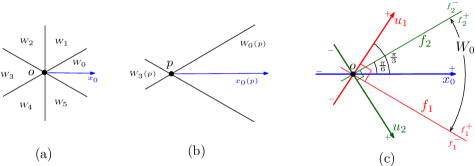
Figure 1: (a) A Partition of the plane into six wedges with common apex at $o$. (b) A translation of $W_{0}$ that moves apex to $p$. The wedge $W_{0}(p)$ is the reflection through $p$ of $W_{3}(p)$ and vise-versa. (c) The wedge $W_{0}$ in $\mathbb{R}^{2}$ is bounded by $f_{1}$ and $f_{2}$. The coordinate axes $u_{1}$ and $u_{2}$ are orthogonal to $f_{1}$ and $f_{2}$.

Consider the $i^{th}$ nearest neighbor $p_{i}$ of $p$. Denote by $L(P\cap W_{l}(p_{i}))$ the list of the points in $P\cap W_{l}(p_{i})$, sorted by increasing order of their $x_{l}$-coordinates (projections). The following lemma provides a key insight. The short proof is omitted (see the full version of the paper in Chapter 6 of the first author’s PhD dissertation [15]).

Lemma 1

Let $p_{i}$ be the $i^{th}$ nearest neighbor of $p$ among a set $P$ of points in $\mathbb{R}^{2}$, and let $W_{l}(p_{i})$ be the wedge of $p_{i}$ that contains $p$. Then point $p$ is among the first $i$ points in $L(P\cap W_{l}(p_{i}))$.

The $k$-nearest neighbor graph ($k$-NNG) of a point set $P$ is constructed by connecting each point in $P$ to all its $k$-nearest neighbors. If we connect each point $p\in P$ to the first $k$ points in the sorted list $L(P\cap W_{l}(p))$, for $l=0,...,5$, we obtain what we call the $k$-Semi-Yao graph ($k$-SYG). Lemma 1 gives a necessary condition for $p_{i}$ to be the $i^{th}$ nearest neighbor of $p$: the point $p$ is among the first $i$ points in $L(P\cap W_{l}(p_{i}))$, where $l$ is such that $p\in W_{l}(p_{i})$. Therefore, the edge set of the $k$-SYG covers the edges of the $k$-NNG. In summary, we have the following.

Lemma 2

The $k$-NNG of a set $P$ of points in $\mathbb{R}^{2}$ is a subgraph of the $k$-SYG of the set $P$.

3 Reporting All $k$-Nearest Neighbors

Here we give a simple method for reporting all the $k$-nearest neighbors via a construction of the $k$-SYG.

Let $C$ be a right circular cone in $\mathbb{R}^{d}$ with opening angle $\theta$ with respect to some given unit vector $v$. Thus $C$ is the set of points $x\in\mathbb{R}^{d}$ such that the angle between $\overrightarrow{ox}$ and $\overrightarrow{v}$ is at most $\theta/2$. The angle between any two rays inside $C$ emanating from the apex $o$ is at most $\theta$. From now on, we assume $\theta\leq\pi/3$.

Now consider a polyhedral cone inscribed in the right circular cone $C$ where the polyhedral cone is formed by the intersection of $d$ distinct half-spaces, bounded by $f_{1},...,f_{d}$, passing through the apex of $C$. Assuming $d$ is arbitrary but fixed, the $d$-dimensional space around the origin $o$ can be tiled by a constant number of polyhedral cones $W_{0},...,W_{c-1}$ [1, 2]. Denote by $C_{l}$ the associated right circular cone of the polyhedral cone $W_{l}$. Let $x_{l}$ be the vector in the direction of the symmetry of $C_{l}$. Denote by $W_{l}(p)$ the translation of the wedge (polyhedral cone) $W_{l}$ where $o$ moves to $p$.

A similar approach and analysis as that in Section 2 can be easily used to state (key) Lemmas 1 and 2 for a set of points in $\mathbb{R}^{d}$.

To construct the $k$-SYG efficiently, we need a data structure to perform the following operation efficiently: For each $p\in P$ and any of its wedges $W_{l}(p)$, $0\leq l\leq c-1$, find the first $k$ points in $L(P\cap W_{l}(p))$. Such an operation can be performed by using range tree data structures. For each wedge $W_{l}$ with apex at origin $o$, we construct an associated $d$-dimensional range tree ${\cal T}_{l}$ as follows.

Consider a particular wedge $W_{l}$ with apex at $o$. The wedge $W_{l}$ is the intersection of $d$ half-spaces $f^{+}_{1},...,f^{+}_{d}$ bounded by $f_{1},...,f_{d}$ (see Figure 1(c)). Let $\hat{u_{j}}$ denote the normal to $f_{j}$ pointing to $f^{+}_{j}$. We define $d$ coordinate axes $u_{j}$, $j=1,...,d$, through $\hat{u_{j}}$, where $\hat{u_{j}}$ gives the respective directions of increasing $u_{j}$-coordinate values.

The range tree ${\cal T}_{l}$ is a regular $d$-dimensional range tree based on the $u_{j}$-coordinates, $j=1,...,d$. The points at level $j$ are sorted at the leaves according to their $u_{j}$-coordinates (for more details about range trees, see Chapter 5 of [4]). Any $d$-dimensional range tree, e.g., ${\cal T}_{l}$, uses $O(n\log^{d-1}n)$ space and can be constructed in time $O(n\log^{d-1}n)$; for any point $r\in\mathbb{R}^{d}$, the points of $P$ inside the query wedge $W_{l}(r)$ whose sides are parallel to $f_{j}$, $j=1,...,d$, can be reported in time $O(\log^{d-1}n+z)$, where $z$ is the cardinality of the set $P\cap W_{l}(r)$ [4].

Now we add a new level to ${\cal T}_{l}$, based on the coordinate $x_{l}$. Let ${\cal C}_{l}(p)$ be the set of the first $k$ points in $L(P\cap W_{l}(p))$. To find ${\cal C}_{l}(p)$ in an efficient time, we use the level $d+1$ of ${\cal T}_{l}$, which is constructed as follows: For each internal node $v$ at level $d$ of ${\cal T}_{l}$, we create a list $L(P(v))$ sorted by increasing order of $x_{l}$-coordinates of the points in $P(v)$. For the set $P$ of $n$ points in $\mathbb{R}^{d}$, the range tree ${\cal T}_{l}$, which now is a $(d+1)$-dimensional range tree, uses $O(n\log^{d}n)$ space and can be constructed in time $O(n\log^{d}n)$.

The following lemma establishes the processing time for obtaining a ${\cal C}_{l}(p)$. The short proof is omitted (see the full version of the paper).

Lemma 3

Given ${\cal T}_{l}$, the set ${\cal C}_{l}(p)$ can be found in time $O(\log^{d}n+k)$.

By Lemma 3, we can efficiently find all the ${\cal C}_{l}(p)$, for all the points $p\in P$. This gives the following lemma.

Lemma 4

Using a data structure of size $O(n\log^{d}n)$, the edges of the $k$-SYG of a set of $n$ points in fixed dimension $d$ can be reported in time $O(n\log^{d}n+kn)$.

Next, suppose we are given the $k$-SYG and we want to report all the $k$-nearest neighbors. Let $E_{p}$ be the set of edges incident to the point $p$ in the $k$-SYG. By sorting these edges in non-decreasing order according to their Euclidean lengths, which can be done in time $O(|E_{p}|\log|E_{p}|)$, we can find the $k$-nearest neighbors of $p$ ordered by increasing distance from $p$. Since the number of edges in the $k$-SYG is $O(kn)$ and each edge $pp^{\prime}$ belongs to exactly two sets $E_{p}$ and $E_{p^{\prime}}$, the time to find all the $k$-nearest neighbors, for all the points $p\in P$, is $\sum_{p}O(|E_{p}|\log|E_{p}|)=O(kn\log n)$.

From the above discussion and Lemmas 2 and 4, the following results.

Theorem 3.1

For a set of $n$ points in fixed dimension $d$, our data structure can report all the $k$-nearest neighbors, in order of increasing distance from each point, in time $O(n\log^{d}n+kn\log n)$. The data structure uses $O(n\log^{d}n+kn)$ space.

4 R$k$NN Queries on Moving Points

We are given a set $P$ of $n$ continuously moving points, where the trajectory of each point in $P$ is a polynomial function of bounded degree $s$. To answer R$k$NN queries on the moving points, we must keep a valid range tree and track all the $k$-nearest neighbors during the motion. This section first shows how to maintain a (ranked-based) range tree, and then provides a KDS for maintenance of the $k$-SYG, which in fact gives a supergraph of the $k$-NNG over time. Using the kinetic $k$-SYG, we can easily maintain all the $k$-nearest neighbors over time. Finally we show how to answer R$k$NN queries on the moving points.

Kinetic RBRT.

Let $u_{j}$, $1\leq j\leq d$, be the coordinate axis orthogonal to the half-space $f_{j}$ of the wedge $W_{l}$, $0\leq l\leq c-1$ (see Figure 1(c)). Abam and de Berg [1] introduced a variant of the range tree, namely the ranked-based range tree (RBRT), which has the following properties. Denote by ${\cal T}_{l}$ the RBRT corresponding to the wedge $W_{l}$.

• ${\cal T}_{l}$ can be described as a set of pairs $\Psi_{l}=\{(B_{1},R_{1}),...,(B_{m},R_{m})\}$ such that:

  • For any two points $p$ and $q$ in $P$ where $q\in W_{l}(p)$, there is a unique pair $(B_{i},R_{i})\in\Psi_{l}$ such that $p\in B_{i}$ and $q\in R_{i}$.

  • For any pair $(B_{i},R_{i})\in\Psi_{l}$, if $p\in B_{i}$ and $q\in R_{i}$, then $q\in W_{l}(p)$ and $p\in W_{l^{\prime}}(q)$; here $W_{l^{\prime}}(q)$ is the reflection of $W_{l}(q)$ through $q$.

  The $\Psi_{l}$ is called a cone separated pair decomposition (CSPD) for $P$ with respect to $W_{l}$. Each pair $(B_{i},R_{i})$ is generated from an internal node $v$ at level $d$ of the RBRT ${\cal T}_{l}$.

• Each point $p\in P$ is in $O(\log^{d}n)$ pairs of $(B_{i},R_{i})$, which means that the number of elements of all the pairs $(R_{i},B_{i})$ is $O(n\log^{d}n)$.

• For any point $p\in P$, all the sets $B_{i}$ (resp. $R_{i}$) where $p\in B_{i}$ (resp. $p\in R_{i}$) can be found in time $O(\log^{d}n)$.

• The set $P\cap W_{l}(p)$ is the union of $O(\log^{d}n)$ sets $R_{i}$, where $p\in B_{i}$.

• When the points are moving, ${\cal T}_{l}$ remains unchanged as long as the order of the points along axes $u_{j}$, $1\leq j\leq d$, remains unchanged.

• When a $u$-swap event occurs, meaning that two points exchange their $u_{j}$-order, the RBRT ${\cal T}_{l}$ can be updated in worst-case time $O(\log^{d}n)$ without rebalancing operations.

4.1 Kinetic $k$-SYG

Here we give a KDS for the $k$-SYG, for any $k\geq 1$, extending [16].

To maintain the $k$-SYG, we must track the set ${\cal C}_{l}(p)$ for each point $p\in P$. So, for each $1\leq i\leq m$, we need to maintain a sorted list $L(R_{i})$ of the points in $R_{i}$ in ascending order according to their $x_{l}$-coordinates over time. Note that each set $R_{i}$ is some $P(v)$, the set of points at the leaves of the subtree rooted at some internal node $v$ at level $d$ of ${\cal T}_{l}$. To maintain these sorted lists $L(R_{i})$, we add a new level to the RBRT ${\cal T}_{l}$; the points at the new level are sorted at the leaves in ascending order according to their $x_{l}$-coordinates. Therefore, in the modified RBRT ${\cal T}_{l}$, in addition to the $u$-swap events, we handle new events, called $x$-swap events, when two points exchange their $x_{l}$-order. The modified RBRT ${\cal T}_{l}$ behaves like a $(d+1)$-dimensional RBRT. From the last property of an RBRT above, when a $u$-swap event or an $x$-swap event occurs, the RBRT ${\cal T}_{l}$ can be updated in worst-case time $O(\log^{d+1}n)$.

Denote by $\ddot{p}_{l,k}$ the $k^{th}$ point in $L(P\cap W_{l}(p))$. To track the sets ${\cal C}_{l}(p)$, for all the points $p\in P$, we need to maintain the following over time.

• A set of $d+1$ kinetic sorted lists $L_{j}(P)$, $j=1,...,d$, and the $L_{l}(P)$ of the point set $P$. We use these kinetic sorted lists to track the order of the points in the coordinates $u_{j}$ and $x_{l}$, respectively.

• For each $B_{i}$, a sorted list $L(B^{\prime}_{i})$ of the points in $B^{\prime}_{i}$, where $B^{\prime}_{i}=\{(p,\ddot{p}_{l,k})|~{}p\in B_{i}\}$. The order of the points in $L(B^{\prime}_{i})$ is according to a label of the second points $\ddot{p}_{l,k}$. This sorted list $L(B^{\prime}_{i})$ is used to answer the following query efficiently: Given a query point $q$ and a $B_{i}$, find all the points $p\in B_{i}$ such that $\ddot{p}_{l,k}=q$.

• The $k^{th}$ point $r_{i,k}$ in the sorted list $L(R_{i})$. We track the values $r_{i,k}$ in order to make necessary changes to the $k$-SYG when an $x$-swap event occurs.

Handling $u$-swap events.

W.l.o.g., let $q\in W_{l}(p)$ before the event. When a $u$-swap event between $p$ and $q$ occurs, the point $q$ moves outside the wedge $W_{l}(p)$; after the event, $q\notin W_{l}(p)$. Note that the changes that occur in the $k$-SYG are the deletions and insertions of the edges incident to $p$ inside the wedge $W_{l}(p)$.

Whenever two points $p$ and $q$ exchange their $u_{j}$-order, we do the following updates.

• We update the kinetic sorted list $L_{j}(P)$. Each swap event in a kinetic sorted list can be handled in time $O(\log n)$.

• We update the RBRT ${\cal T}_{l}$ and if a point is deleted or inserted into a $B_{i}$, we update the sorted list $L(B^{\prime}_{i})$. Since each insertion/deletion to $L(B^{\prime}_{i})$ takes $O(\log n)$ time, and since each point is in $O(\log^{d}n)$ sets $B_{i}$, this takes $O(\log^{d+1}n)$ time.

• We update the values of $r_{i,k}$. After updating the RBRT ${\cal T}_{l}$, point $q$ might be inserted or deleted from some $R_{i}$ and change the values of $r_{i,k}$. So, for all $R_{i}$ where $q\in R_{i}$, before and after the event, we do the following. We check whether the $x_{l}$-coordinate of $q$ is less than or equal to the $x_{l}$-coordinate of $r_{i,k}$; if so, we take the successor or predecessor point of $r_{i,k}$ in $L(R_{i})$ as the new value for $r_{i,k}$. This takes $O(\log^{d+1}n)$ time.

• We query to find ${\cal C}(p)$. By Lemma 3, this takes $O(\log^{d}n+k)$ time.

• If we get a new value for $\ddot{p}_{l,k}$, we update all the sorted lists $L(B^{\prime}_{i})$ such that $p\in B_{i}$. This takes $O(\log^{d+1}n)$ time.

Considering the complexity of each step above, and assuming the trajectory of each point is a bounded degree polynomial, the following results.

Lemma 5

Our KDS for maintenance of the $k$-SYG handles $O(n^{2})$ $u$-swap events, each in worst-case time $O(\log^{d+1}n+k)$.

Handling $x$-swap events.

When an $x$-swap event between two consecutive points $p$ and $q$ with $p$ preceding $q$ occurs, it does not change the elements of the pairs $(B_{i},R_{i})$ of the CSPD $\Psi_{l}$. Such an event changes the $k$-SYG if both $p$ and $q$ are in the same $W_{l}(w)$, for some $w\in P$, and $w_{l,k}=p$.

We apply the following updates to our KDS when two points $p$ and $q$ exchange their $x_{l}$-order.

1. We update the kinetic sorted list $L_{l}(P)$; this takes $O(\log n)$ time.

2. We update the RBRT ${\cal T}_{l}$, which takes $O(\log^{d+1}n)$ time.

3. We find all the sets $R_{i}$ where both $p$ and $q$ belong to $R_{i}$ and such that $r_{i,k}=p$. Also, we find all the sets $R_{i}$ where $r_{i,k}=q$. This takes $O(\log^{d}n)$ time.

4. For each $R_{i}$, we extract all the pairs $(w,\ddot{w}_{l,k})$ from the sorted lists $L(B^{\prime}_{i})$ such that $\ddot{w}_{l,k}=p$. Note that each change to the pair $(w,\ddot{w}_{l,k})$ is a change to the $k$-SYG.

5. For each $w$, we update all the sorted lists $L(B^{\prime}_{i})$ where $(w,\ddot{w}_{l,k})\in B^{\prime}_{i}$: we replace the previous value of $\ddot{w}_{l,k}$, which is $p$, by the new value $q$.

Denote by $\chi_{k}$ the number of exact changes to the $k$-SYG  of a set of moving points over time. For each found $R_{i}$, the fourth step takes $O(\log n+\xi_{i})$ time, where $\xi_{i}$ is the number of pairs $(w,\ddot{w}_{l,k})$ such that $\ddot{w}_{l,k}=p$. For all these $O(\log^{d}n)$ sets $R_{i}$, this step takes $O(\log^{d+1}n+\sum_{i}\xi_{i})$ time, where $\sum_{i}\xi_{i}$ is the number of exact changes to the $k$-SYG when an $x$-swap event occurs. Therefore, for all the $O(n^{2})$ $x$-swap events, the total processing time for this step is $O(n^{2}\log^{d+1}n+\chi_{k})$.

The processing time for the fifth step is a function of $\chi_{k}$. For each change to the $k$-SYG, this step spends $O(\log^{d+1}n)$ time to update the sorted lists $L(B^{\prime}_{i})$. Therefore, the total processing time for all the $x$-swap events in this step is $O(\chi_{k}*\log^{d+1}n)$.

From the above discussion and an upper bound for $\chi_{k}$ in Lemma 6, Lemma 7 results. The proof of Lemma 6 is omitted (see the full version of the paper).

Lemma 6

The number of changes to the $k$-SYG of a set of $n$ moving points, where the trajectory of each point is a polynomial function of at most constant degree $s$, is $\chi_{k}=O(\phi(s,n)*n)$.

Lemma 7

Our KDS for maintenance of the $k$-SYG handles $O(n^{2})$ $x$-swap events with a total cost of $O(\phi(s,n)*n\log^{d+1}n)$.

From Lemmas 5 and 7, the following theorem results.

Theorem 4.1

For a set of $n$ moving points in $\mathbb{R}^{d}$, where the trajectory of each point is a polynomial function of at most constant degree $s$, our $k$-SYG KDS uses $O(n\log^{d+1}n)$ space and handles $O(n^{2})$ events with a total cost of $O(kn^{2}+\phi(s,n)*n\log^{d+1}n)$.

4.2 Kinetic All $k$-Nearest Neighbors

Given a KDS for maintenance of the $k$-SYG (from Theorem 4.1), a supergraph of the $k$-NNG, this section shows how to maintain all the $k$-nearest neighbors over time. For maintenance of the $k$-nearest neighbors of each point $p\in P$, we only need to track the order of the edges incident to $p$ in the $k$-SYG according to their Euclidean lengths. This can easily be done by using a kinetic sorted list. The following theorem summarizes the complexity of our kinetic approach. The proof is omitted (see the full version of the paper).

Theorem 4.2

For a set of $n$ moving points in $\mathbb{R}^{d}$, where the trajectory of each point is a polynomial of at most constant degree $s$, our KDS for maintenance of all the $k$-nearest neighbors, ordered by distance from each point, uses $O(n\log^{d+1}n+kn)$ space and $O(n\log^{d+1}n+kn\log n)$ preprocessing time. Our KDS handles $O(\phi(s,n)*n^{2})$ events, each in $O(\log n)$ amortized time.

4.3 R$k$NN Queries

Suppose we are given a query point $q\notin P$ at some time $t$. To find the reverse $k$-nearest neighbors of $q$, we seek the points in $P\cap W_{l}(q)$ and find ${\cal C}_{l}(q)$, the set of the first $k$ points in $L(P\cap W_{l}(q))$. The set $\cup_{l}{\cal C}_{l}(q)$ contains $O(k)$ candidate points for $q$ such that $q$ might be one of their $k$-nearest neighbors. In time $O(\log^{d}n)$ we can find a set of $R_{i}$ where $P\cap W_{l}(q)=\sum_{i}R_{i}$. From Lemma 3, and since we have sorted lists $L(R_{i})$ at level $d+1$ of ${\cal T}_{l}$, the $O(k)$ candidate points for the query point $q$ can be found in worst-case time $O(\log^{d}n+k)$. Now we check whether these candidate points are the reverse $k$-nearest neighbors of the query point $q$ at time $t$ or not; this can be easily done by application of Theorem 4.2, which in fact maintain the $k^{th}$ nearest neighbor $p_{k}$ of each $p\in P$. Therefore, checking a candidate point can be done in $O(1)$ time by comparing distance $|pq|$ to distance $|pp_{k}|$. This implies that checking which elements of ${\cal C}_{l}(q)$, for $l=0,...,c-1$, are reverse $k$-nearest neighbors of the query point $q$ takes time $O(k)$.

If a query arrives at a time $t$ that is simultaneous with the time when one of the $O(\phi(s,n)*n^{2})$ events occurs, our KDS first spends amortized time $O(\log n)$ to handle the event, and then spends time $O(\log^{d}n+k)$ to answer the query. Thus we have the following.

Theorem 4.3

Consider a set $P$ of $n$ moving points in $\mathbb{R}^{d}$, where the trajectory of each one is a bounded-degree polynomial. The number of reverse $k$-nearest neighbors for a query point $q\notin P$ is $O(k)$. Our KDS uses $O(n\log^{d+1}n+kn)$ space, $O(n\log^{d+1}n+kn\log n)$ preprocessing time, and handles $O(\phi(s,n)*n^{2})$ events. At any time $t$, an R$k$NN query can be answered in time $O(\log^{d}n+k)$. If an event occurs at time $t$, the KDS spends amortized time $O(\log n)$ on updating itself.

5 Discussion

In the kinetic setting, where the trajectories of the points are polynomials of bounded degree, to answer the R$k$NN queries over time we have provided a KDS for maintenance of all the $k$-nearest neighbors. Our KDS is the first KDS for maintenance of all the $k$-nearest neighbors in $\mathbb{R}^{d}$, for any $k\geq 1$. It processes $O(\phi(s,n)*n^{2})$ events, each in amortized time $O(\log n)$. An open problem is to design a KDS for all $k$-nearest neighbors that processes less than $O(\phi(s,n)*n^{2})$ events.

Arya et al. [3] have a kd-tree implementation to approximate the nearest neighbors of a query point that is in use by practitioners [11] who have found challenging to implement the theoretical algorithms [5, 10, 12, 18]. Since to report all the $k$-nearest neighbors ordered by distance from each point our method uses multidimensional range trees, which can be easily implemented, we believe our method may be useful in practice.

Acknowledgments.

We thank Timothy M. Chan for his helpful comments and suggestions.

References

- [1] Abam, M.A., de Berg, M.: Kinetic spanners in . Discrete & Computational Geometry 45(4), 723–736 (2011)
- [2] Agarwal, P.K., Kaplan, H., Sharir, M.: Kinetic and dynamic data structures for closest pair and all nearest neighbors. ACM Transactions on Algorithms 5, 4:1–37 (2008)
- [3] Arya, S., Mount, D.M., Netanyahu, N.S., Silverman, R., Wu, A.Y.: An optimal algorithm for approximate nearest neighbor searching in fixed dimensions. Journal of the ACM 45(6), 891–923 (1998)
- [4] Berg, M.d., Cheong, O., Kreveld, M.v., Overmars, M.: Computational Geometry: Algorithms and Applications. Springer-Verlag TELOS, Santa Clara, CA, USA, 3rd edn. (2008)
- [5] Callahan, P.B., Kosaraju, S.R.: A decomposition of multidimensional point sets with applications to -nearest-neighbors and -body potential fields. Journal of the ACM 42(1), 67–90 (1995)
- [6] Chan, T.M.: On levels in arrangements of curves, ii: A simple inequality and its consequences. Discrete & Computational Geometry 34(1), 11–24 (2005)
- [7] Chan, T.M.: On levels in arrangements of curves, iii: further improvements. In: Proceedings of the 24th annual Symposium on Computational Geometry (SoCG ’08). pp. 85–93. ACM, New York, NY, USA (2008)
- [8] Cheema, M.A., Zhang, W., Lin, X., Zhang, Y., Li, X.: Continuous reverse k nearest neighbors queries in euclidean space and in spatial networks. The VLDB Journal 21(1), 69–95 (2012)
- [9] Cheong, O., Vigneron, A., Yon, J.: Reverse nearest neighbor queries in fixed dimension. International Journal of Computational Geometry and Applications 21(02), 179–188 (2011)
- [10] Clarkson, K.L.: Fast algorithms for the all nearest neighbors problem. In: Proceedings of the 24th Annual Symposium on Foundations of Computer Science (FOCS ’83). pp. 226–232. IEEE Computer Society, Washington, DC, USA (1983)
- [11] Connor, M., Kumar, P.: Fast construction of -nearest neighbor graphs for point clouds. IEEE Transactions on Visualization and Computer Graphics 16(4), 599–608 (2010)
- [12] Dickerson, M.T., Eppstein, D.: Algorithms for proximity problems in higher dimensions. International Journal of Computational Geometry and Applications 5(5), 277–291 (1996)
- [13] Korn, F., Muthukrishnan, S.: Influence sets based on reverse nearest neighbor queries. In: Proceedings of the 2000 ACM SIGMOD International Conference on Management of Data (SIGMOD ’00). pp. 201–212. ACM, New York, NY, USA (2000)
- [14] Maheshwari, A., Vahrenhold, J., Zeh, N.: On reverse nearest neighbor queries. In: Proceedings of the 14th Canadian Conference on Computational Geometry (CCCG ’02). pp. 128–132 (2002)
- [15] Rahmati, Z.: Simple, Faster Kinetic Data Structures. Ph.D. thesis, University of Victoria (2014), http://zahedrahmati.com
- [16] Rahmati, Z., Abam, M.A., King, V., Whitesides, S.: Kinetic data structures for the Semi-Yao graph and all nearest neighbors in . In: Proceedings of the 26th Canadian Conference on Computational Geometry (CCCG ’14) (2014)
- [17] Rahmati, Z., King, V., Whitesides, S.: Kinetic data structures for all nearest neighbors and closest pair in the plane. In: Proceedings of the 29th Symposium on Computational Geometry (SoCG ’13). pp. 137–144. ACM, New York, NY, USA (2013)
- [18] Vaidya, P.M.: An O() algorithm for the all-nearest-neighbors problem. Discrete & Computational Geometry 4(2), 101–115 (1989)