Stability of cellular automata trajectories revisited:
branching walks and Lyapunov profiles

April 11, 2016

Abstract.

We study non-equilibrium defect accumulation dynamics on a cellular automaton trajectory: a branching walk process in which a defect creates a successor on any neighborhood site whose update it affects. On an infinite lattice, defects accumulate at different exponential rates in different directions, giving rise to the Lyapunov profile. This profile quantifies instability of a cellular automaton evolution and is connected to the theory of large deviations. We rigorously and empirically study Lyapunov profiles generated from random initial states. We also introduce explicit and computationally feasible variational methods to compute the Lyapunov profiles for periodic configurations, thus developing an analogue of Floquet theory for cellular automata.

2010 Mathematics Subject Classification: 60K35, 37B15.

Key words and phrases: asymptotic shape, branching walk, cellular automaton, doubly periodic configuration, large deviations, Lyapunov exponent, percolation, stability.

1 Introduction

Quantifying instability in physical systems and in mathematical models is a long-standing problem in nonlinear science, beginning with Lyapunov’s pioneering work at the end of 19th century. Lyapunov discovered that the basic quantities are exponential rates which, when positive, measure divergence from an unstable trajectory. In this paper, we elaborate on the well-known fact that instabilities often do not affect all components of a system to the same extent; more precisely, we study how fast defects may spread among these components, which we assume are spatially distributed. In the process, we establish connections with large deviation theory, a branch of probability theory that studies exponentially small probabilities of “rare” events that do not conform to the “typical” scenario. In our models, the defects accumulate in space as a system of random walks, whose large deviation rates then determine Lyapunov instability. This point of view is not only useful when the dynamics starts at a random initial state, but also in periodic states with no randomness at all.

While our approach could work for other many-component systems, we chose cellular automata (CA) as our platform. These deterministic dynamical systems are spatially and temporally discrete, with a fixed local update rule that mandates that a new state at the next tick of a clock depends only on a finite number of neighboring states. In addition, each spatial location (playing the role of a component or a degree of freedom) can be occupied with one of only finitely many states — for simplicity, we will only consider binary CA, in which a site either takes the state $0$ or the state $1$. This setting minimizes technical considerations, which however remain a considerable challenge. It also facilitates the development of a computational approach, which has become an indispensable element of stability research in many fields, but is particularly well-suited for CA. Consequently, our conclusions are based both on large-scale calculations and on rigorous mathematical arguments, the latter largely probabilistic.

Let us consider a binary CA that is evolved from an initial state $\xi_{0}$, generating a trajectory $\xi_{t}$, $t=0,1,\ldots$. For instance, the CA known as Rule 22 or Exactly 1 [GG4], whose sites are integers in ${\mathbb{Z}}$, is governed by the update rule dictating that the state at $x\in{\mathbb{Z}}$ is $1$ at time $t\geq 1$ if and only if exactly one of states at its three neighboring sites $x-1$, $x$ and $x+1$ was $1$ at the previous time step. How stable is a CA trajectory? By analogy with continuous dynamical systems, the idea is to measure the effect of a small perturbation of $\xi_{0}$ on the evolution at later times. In his classic work, Wolfram [Wol1] considered damage spreading, that is, growth of the set of affected sites in $\xi_{t}$ when a few sites in $\xi_{0}$ are flipped. In one dimension, there are two directions of propagation; when the maximum extent of damage progresses linearly the two slopes are called Lyapunov exponents as they measure the exponential divergence in distance between the original and perturbed states in the appropriate metric. This concept was developed further from computational and theoretical perspectives in [Gra1, Gra2, She, CK, FMM, Tis1, Tis2].

Damage spreading is possibly the simplest approach but it gives no indication on the rate of divergence within a bounded region; in particular it has nothing to say on the CA evolution on finite sets. Thus a different tool was introduced by Bagnoli et al. [BRR], based on the fact that Lyapunov exponents in continuous dynamical systems can also be given locally through the eigenvalues of the governing Jacobian. The Boolean derivative introduced in [Vic1] is used in [BRR] as the analogue for the Jacobian, which leads to the branching walk dynamics of defects that we now informally describe. Recall that a trajectory $\xi_{t}$ of a CA is fixed. Assume a defect is present at a site $y$ at time $t$. That defect looks into each of its neighborhood sites $x$ to check whether flipping the state $\xi_{t}$ at $y$ would produce a different state at $x$ than assigned by $\xi_{t+1}$; if so, the defect produces a successor at $x$. Each defect may produce more than one successor (hence the term “branching”) and acts independently of other defects. The exponential rate of accumulation of such defects is called the maximal Lyapunov exponent (MLE). The authors of [BRR] envision this as an equilibrium theory: they measure the accumulation on a finite circle of sites after a long time (much larger than the length of the circle) has elapsed. Due to the resulting spatial translation invariance, there is only one rate of accumulation, and the meaning of the word maximal is unclear, except to distinguish the notion from the one arising from damage spreading; however, the present setting provides an ex post facto justification of this term.

In this paper we continue the study initiated in [BG] of the non-equilibrium version of defect branching walk dynamics. As the defects spread on an infinite lattice, there is substantial spatial variation in their accumulation; the exponential rates of spread in all space-time directions are collected into a function we call the Lyapunov profile. For example, a one-dimensional Lyapunov profile $L=L(\alpha)$ roughly gives, for a real number $\alpha$, the exponential rate of accumulation on the line $x=\alpha t$ (see Fig. 1.1 for a few examples, including Rule 22). There is some conceptual similarity between this object and the Lyapunov spectrum in multidimensional smooth dynamical systems, whereby the spectrum of the Jacobian accounts for perturbations in all directions in both the input and the output. In the discrete CA configuration space there is essentially one way to make an infinitesimal perturbation in the input (assuming irreducibility), but the effect can be quite different in different directions of the output. Moreover, we empirically observe that typically the direction with the maximal effect has the profile height that is close to the MLE of [BRR].

We emphasize that the dynamics of branching defects does not alter the trajectory $\xi_{t}$ but instead uses it as an environment for its evolution. It is thus a kind of second-class dynamics akin to the ones that percolate and create periodic structures in [GH], and to the “slave” synchronization rules of [BER]. In fact, the set of sites that contain at least one defect evolves as a four-state CA, which we refer to as the defect percolation CA, and which is conceptually very similar to the rules studied in [GH]. One property that substantially facilitates the analysis is that our dynamics are monotone — adding defects only results in more of them later on — a property that fails to hold for Wolfram’s damage spreading. We call the asymptotic rate of defect spread, typically equal to the set on which the Lyapunov profile differs from $-\infty$, the defect shape. The Lyapunov profiles thus simultaneously provide information on the spatial reach and local accumulation resulting from a defect perturbation. The defect shape does not have an a priori relation to the (appropriately scaled) damaged set; as we will see in Section 3, it can be larger or smaller.

The most important initial state $\xi_{0}$ for the CA analysis is the uniform product measure, that is, one in which the probability of a $0$ or a $1$ at any site is independently $1/2$. Indeed, this random configuration is, in a way, one in which all configurations are equally likely. The trajectory $\xi_{t}$ then determines a space-time random field for defect dynamics, resulting in a branching random walk process. The study of such processes in an independent space-time random environment (e.g., [Big, BNT]) is a well-established subfield of the large deviations theory [DZ, RS]. The main idea is that the resulting profiles are given by a variational method: the process seeks the most advantageous option for accumulation at a spatial location; in general, the search space can have a very high dimension. Our defect accumulation dynamics evolves in a highly correlated random field, even when the uniform product measure is invariant [GH], and extending large deviation techniques is an extraordinary challenge. We thus rely mostly on empirical methods to analyze nontrivial cases with random initialization. Notably, we observe that detectable dependence of MLE on the initial CA density is connected to the dramatic advantage of the defect percolation as compared to the damage spreading.

The other extreme are spatially periodic initial states, which after a transient “burn-in” time interval must become also temporally periodic. Study of the stability of periodic solutions of dynamical systems also has a long history, and is known as Floquet theory; see e.g. [Moo] for a recent perspective. We are able to develop a fairly complete analogue for CA dynamics, based on large deviations for finite Markov chains [DZ, RS]. These methods work particularly well under the irreducibility assumption, in which case the Lyapunov profile is given by a one-dimensional variational problem. We give several examples in Section 6.2, including the profile for the Rule 110 ether [Coo]. We also introduce direct methods to determine the defect shape, related to convex transforms that originate from crystallography.

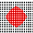
(a)

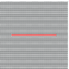
(b)

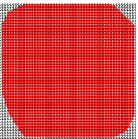
(c)

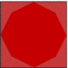
(d)

Figure 6.2: Examples of defect shapes for Tot 1 ((a) and (b)), Tot 3 (c), and Tot 7 (d) rules.

Lyapunov profiles encapsulate a lot of information on the stability of CA trajectory, but not all of it. For example, many rules, such as Rule 22, develop holes in the set of defect sites (see Fig. 1.1) due to stable updates, that is, configurations whose updates are insensitive to perturbations at a single site. Thus the defect density profile, a function that gives the density of defect sites in a given space-time direction, is of interest. Although there is no known a priori reason, density profiles of CA trajectories are typically constant on their support [GG4, GG5]; we observe the same here (see Fig. 3.1), although non-constant density profiles do occur, for example, due to reducibility (e.g., Tot 7 example in Fig. 6.2).

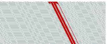
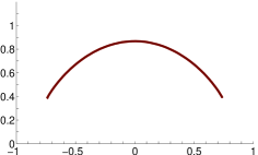
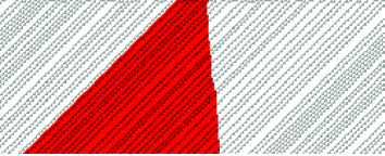
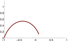
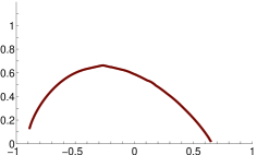
Figure 1.1: Evolution of defect percolation CA up to time $100$ (red sites are those that contain at least one defect) and empirical Lyapunov profiles at time $10^{5}$ for rules 7, 22, 38, and 110.

These profiles encapsulate the exponential accumulation rate vs. space-time direction.

We give formal definitions and some general results in Section 2, after which we focus on elementary CA [Wol1], the $256$ one-dimensional, three-neighbor rules that have long been considered the primary testing ground for any CA theory, including stability analysis (e.g., [BRR]). Due to their wide acceptance, we use the Wolfram’s serial numbers [Wol1] as nomenclature; the web site [Wol2] is particularly useful for a quick reference. Section 4 includes a comprehensive discussion on elementary CA defect dynamics from the uniform product initial state. We also consider two-dimensional rules (Sections 5 and 6.1), where we restrict to totalistic rules whose update only depends on the neighborhood count.

We conclude this section with a few illustrative examples and a brief discussion on how our approach relates to other complexity measures of CA rules. Fig. 1.1 depicts a sample defect percolation evolution for four elementary CA, together with approximate Lyapunov profiles. In all cases $\xi_{0}$ is the uniform product measure and the initial set of defects is an interval of $21$ sites. The first example is Rule 7, one of many rules with degenerate profiles that are typically caused by persistent moving obstacles that defects cannot cross (see Table LABEL:ECA-marginal). Next is Rule 22, a classic chaotic rule for which it appears, at first glance, that the defect percolation has the same asymptotics as damage spreading [Gra2], but we will present evidence that this is not the case (see Fig. 3.1). Next, Rule 38 is the simplest stripes rule (see Section 3) in which the initial state creates a quenched random environment for the branching walks, and thus the dynamics is conceptually similar to one on a random tessellation [BD]. Much about the resulting dynamics can be proved (see Prop. 4.6). The final example is Rule 110, which famously creates a periodic ether for interaction between various types of gliders [Coo]. Whether the density of gliders approaches zero is unknown (see [LN] for positive evidence), and thus it is even less clear whether the Lyapunov profile approaches the one obtained by starting from the ether. The latter profile can be characterized by an explicit variational formula (see Section 6.2.3).

There have been many attempts to classify CA through complexity, going back to [Wol1]; see [MSZ, Mar, ZV] for recent reviews. The original Wolfram classification into four classes, uniform, periodic, chaotic and complex, often simply referred to by numerals 1–4, is still in wide use [Mar], despite considerable ambiguity in many interesting cases [MSZ]; for example, the intriguing Rule 106 (or its edge version EEED [GG5]) could be called chaotic or complex. Much of the literature has attempted to condense the complexity properties of a CA rule into a single number, although it is unclear if a linear ordering of CA by complexity provides the most insight; see [ZV] and [Mar] for some “competing” measures and resulting classifications. Our paper underscores this point by instead assigning a function to every CA rule, as in the right panels of Figure 1.1. This leads to a natural division of rules into three classes, which can in the case of elementary CA be described as follows: collapsing rules for which the defects die out (e.g., rules 0 and 40); marginal rules whose Lyapunov profile is a single “stick,” as is for Rule 7 in Figure 1.1; and expansive rules which generate exponential accumulation of defects on a linearly growing set, as in the other three cases of Figure 1.1.

One may intuitively expect that rules that have, by some measure, large complexity are the expansive ones. As tends to be the case, this rule of thumb is useful, but is not a perfect predictor, as we now briefly illustrate on elementary CA. To be definite, we use Table 2 in [Mar] as Wolfram’s classification. The 8 uniform (class 1) rules are exactly the 8 rules in Table 4.2 and are therefore all collapsing. At the other extreme, the 11 chaotic (class 3) and 4 complex (class 4) rules are all expansive (see Table 4.4). However, there are expansive elementary CA which are classified as periodic (class 2). These are the stripes rules (of which Rule 38 from Figure 1.1 is an example), which are in a sense in their own class: expansive but simple enough to be at least partly amenable to mathematical analysis. On the other side, there are two marginal rules, 73 and 94, that are sometimes classified as periodic [Mar] and sometimes as complex [ZV], and stand out in our analysis as well in that the height of their profile is unusually difficult to estimate. Finally, the three additional collapsing rules identified in Table 4.5 are just barely such, as discussed in Section 4.5. The exceptional rules mentioned in this paragraph — among which the remaining eight glider rules in Table 4.5 can also be counted — are all worth further study.

2 Definitions and basic results

In this paper we only consider binary CA, leaving the discussion of larger state spaces to our subsequent work. Thus, our object of study is a cellular automaton on the $d$-dimensional integer lattice ${\mathbb{Z}}^{d}$ with state space $\{0,1\}$ that is given by the finite ordered neighborhood ${\mathcal{N}}\subset{\mathbb{Z}}^{d}$ and the (local) update function of $|{\mathcal{N}}|$ variables: $\phi:\{0,1\}^{|{\mathcal{N}}|}\to\{0,1\}$. For a string $\vec{s}\in\{0,1\}^{|{\mathcal{N}}|}$ we also write $\vec{s}\mapsto s^{\prime}$ instead of $\phi(\vec{s})=s^{\prime}$. We call an update $\vec{s}\mapsto s^{\prime}$ stable if $\vec{s}_{1}\mapsto s^{\prime}$ for every $\vec{s}_{1}$ that differs from $\vec{s}$ in only one state.

The neighborhood of a point $x\in{\mathbb{Z}}^{d}$ is the translation ${\mathcal{N}}_{x}=x+{\mathcal{N}}$, ordered the same way as ${\mathcal{N}}$. The global function $\Phi:\{0,1\}^{{\mathbb{Z}}^{d}}\to\{0,1\}^{{\mathbb{Z}}^{d}}$ is given as follows. For arbitrary $\eta\in\{0,1\}^{{\mathbb{Z}}^{d}}$, and $x\in{\mathbb{Z}}^{d}$, let $\eta|_{{\mathcal{N}}_{x}}$ be the vector of $|{\mathcal{N}}|$ entries given by values of $\eta$ on ${\mathcal{N}}_{x}$, listed in the order of sites in ${\mathcal{N}}_{x}$. The function $\phi$ applied to this vector provides the value of $\Phi(\eta)$ at $x$; in symbols,

$$\Phi(\eta)(x)=\phi(\eta|_{{\mathcal{N}}_{x}}).$$

We denote by $\xi_{t}(x)=\xi(x,t)$, $x\in{\mathbb{Z}}^{d}$, $t\in{\mathbb{Z}}_{+}$, a trajectory of the CA, starting from a fixed initial state $\xi_{0}$, which can be deterministic or random. That is, $\xi_{t}$ is defined recursively by iteration of $\Phi$: $\xi_{t+1}=\Phi(\xi_{t})$ for $t\geq 0$.

2.1 Lyapunov profiles

We begin by defining the branching walk dynamics that measures propagation of perturbations; see e.g. [Big, BNT] for probabilistic analysis of branching random walk. The defect configuration $\Delta_{t}(x)=\Delta(x,t)\in{\mathbb{Z}}_{+}$ describes the distribution of defects. Informally, for every $x\in{\mathbb{Z}}^{d}$, $y\in{\mathcal{N}}_{x}$, and every defect counted into $\Delta_{t}(y)$, $\Delta_{t+1}(x)$ is increased by 1 if applying the CA rule on the configuration $\xi_{t}$ that is perturbed at $y$ results in a perturbation at $x$.

More formally, for a configuration $\eta\in\{0,1\}^{{\mathbb{Z}}^{d}}$, and $y\in{\mathbb{Z}}^{d}$, the perturbation of $\eta$ at $y$ is the configuration $\eta^{(y)}$ defined by

$$\eta^{(y)}(x)=\begin{cases}1-\eta(y)&x=y\\ \eta(x)&\text{otherwise}\end{cases}$$

Further, $\text{\tt change}_{t}$ collects the information about effects of perturbations at time $t$, and is essentially the Boolean derivative [Vic1],

$$\text{\tt change}_{t}(y,x)=\mathbbm{1}(\Phi(\xi_{t}^{(y)})(x)\neq\xi_{t+1}(x)).$$

(Here, $\mathbbm{1}$ is the indicator function, which gives the value $1$ or $0$ whenever its logical argument is true or false, respectively.) Then,

$$\Delta_{t+1}(x)=\sum_{y\in{\mathcal{N}}_{x}}\text{\tt change}_{t}(y,x)\Delta_{t}(y).$$

Again, $\Delta_{0}$ is a fixed configuration, which we will always assume is nonzero with (possibly large) finite support. We call $(\xi_{t},\Delta_{t})$ the defect accumulation dynamics, matching the definition in [BRR].

The configuration $\delta_{t}$ given by $\delta_{t}(x)=\mathbbm{1}(\Delta_{t}(x)>0)$ induces a CA evolution $(\xi_{t},\delta_{t})$, which we call the defect percolation CA. In this four-state rule, a defect at $y$ spreads into a neighboring site $x$ if a change of the state of $\xi_{t}$ at $y$ affects the state at $x$ at the next time step. Therefore, $\delta_{t}$ is an oriented percolation dynamics on the original space-time CA configuration $\xi_{t}$; it is affected by the original CA evolution, leaving it unaffected in return. Thus it plays a similar role to the percolation process in [GH] that governs disorder-resistance. Another example are the “second-class” or “slave” processes that control synchronization in [BER]. As convenient, we often interpret $\delta_{t}$ as subset of ${\mathbb{Z}}^{d}$, determined by its support.

We define the Lyapunov profile to be the function $L:{\mathbb{R}}^{d}\to\{-\infty\}\cup[0,\infty)$ given for $\alpha\in{\mathbb{R}}^{d}$ by

(2.1) $$L(\alpha)=\lim_{\epsilon\downarrow 0}\limsup_{t\to\infty}\frac{1}{t}\log\left(\sum_{x:||x/t-\alpha||<\epsilon}\Delta(x,t)\right),$$

where the norm is Euclidean (or, equivalently, any other). Informally,

$$\Delta(t\alpha,t)\approx e^{L(\alpha)t},$$

so that in the space-time direction $\alpha$ the defects accumulate at the exponential rate $L(\alpha)$. We call the Lyapunov profile $L$ proper if replacing $\limsup$ with $\liminf$ in (2.1) results in the same limit $L(\alpha)$ for all $\alpha$.

It is easy to see that the limit in (2.1) exists as either a nonnegative finite number or $-\infty$, and that one may replace the sum with maximum. It is also clear that $L(\alpha)=-\infty$ when $\alpha$ is outside $\text{co}({\mathcal{N}})$, the convex hull of ${\mathcal{N}}$. Further, $L(\alpha)\leq\log|{\mathcal{N}}|$ for all $\alpha$ and $L$ is upper semicontinuous. The maximal Lyapunov exponent (MLE) is then defined to be

(2.2) $$\lambda=\max_{\alpha}L(\alpha).$$

An $\alpha$ at which the maximum in (2.2) is achieved is called a MLE direction, and is a space-time direction with the fastest growth of the number of defects. See [BRR] for a different definition of the MLE, and [BD] for a discussion in a more general context. We empirically observe that our concept of MLE is close to that of [BRR] when the initial state is uniform product measure.

A binary CA is additive when the local map $\phi$ adds all its arguments modulo $2$. In this case the Lyapunov profile is proper and independent of $\xi_{0}$ and $\Delta_{0}$. As it depends only on the neighborhood ${\mathcal{N}}$, we denote the resulting Lyapunov profile by $L_{\mathcal{N}}$. By elementary large deviations [DZ, RS], we can give it as a variational formula. For $y\in{\mathbb{R}}^{d}$, let

$$\Lambda(y)=\sum_{x\in{\mathcal{N}}}\exp(\langle y,x\rangle).$$

Then $L_{\mathcal{N}}$ is given by the Legendre transform

$$L_{\mathcal{N}}(\alpha)=\inf_{y}\left(-\langle y,\alpha\rangle+\Lambda(y)\right).$$

Furthermore, $\lambda(\alpha)=\log|{\mathcal{N}}|$ with the unique MLE direction given by the average of ${\mathcal{N}}$: $|{\mathcal{N}}|^{-1}\sum_{x\in{\mathcal{N}}}x.$ For example, Rule 150 is the one-dimensional additive CA with ${\mathcal{N}}=\{0,\pm 1\}$ and has

$$L(\alpha)=L_{\mathcal{N}}(\alpha)=\log\left(1+\alpha_{0}+\frac{1}{\alpha_{0}}\right)-\alpha\log\alpha_{0},\text{ where }\alpha_{0}=\frac{\alpha+\sqrt{4-3\alpha^{2}}}{2(1-\alpha)},$$

with MLE $\lambda=\log 3$ and MLE direction $0$. Clearly, for any CA with neighborhood ${\mathcal{N}}$, and any initialization $\xi_{0}$ and $\Delta_{0}$,

$$L(\alpha)\leq L_{\mathcal{N}}(\alpha).$$

In this sense, the additive CA are the most unstable.

We also remark that, for additive rules, the theorem due to Badahur and Rao (see Section 3.7 of [DZ]) implies that for a fixed $\epsilon$ the $t$-limit in (2.1) exists and the convergence rate is $\mathcal{O}(t^{-1}\log t)$. Periodic cases (Section 6.2) and chaotic rules with strong mixing properties (e.g., rules 22, 30, and 106 among elementary CA) appear to exhibit similarly fast convergence, while many other cases progress more slowly due to the fact that $\xi_{t}$ itself does so. In our empirical Lyapunov profile plots from random initial states, we choose $t=10^{5}$ and $\epsilon=4\cdot 10^{-3}$; we do not add the huge numbers of defects using exact integer arithmetic but instead use double precision to compute their logarithms using this formula for $0<B\leq A$:

$$\log(A+B)=\log A+\log(1+\exp(\log B-\log A)).$$

2.2 Density profiles and defect shapes

Due to stable updates, the set of defect sites often has holes that are invisible in the Lyapunov profile $L$. To capture this information, we introduce the function $\rho=\rho(\alpha)$ that gives the proportion of defect sites in the direction $\alpha\in{\mathbb{R}}^{d}$, that is, on the rays $x=\alpha t$. Formally, we call $\rho$ the defect density profile if, as $T\to\infty$, the measures given by properly scaled point-masses at $x/t$, for $(x,t)$ with $t\leq T$ and $\delta(x,t)=1$, converge to $\rho$ in the following sense:

(2.3) $$\frac{2^{d}}{T^{d+1}}\sum_{(x,t):t\leq T,\delta(x,t)=1}\psi(x/t)\xrightarrow[T\to\infty]{}\int_{{\mathbb{R}}^{d}}\rho(\alpha)\psi(\alpha)\,d\alpha,$$

for any test function $\psi\in{\mathcal{C}}_{c}({\mathbb{R}}^{d})$. (Note that this convergence is in the weak^∗-topology used in functional analysis.) The scaling is chosen so that, when $\delta\equiv 1$, $\rho\equiv 1$. See [GG2, GG4, GG5] for other examples of density profiles.

Furthermore, we define the defect shape $W$ to be the closed subset ${\mathbb{R}}^{d}$ obtained by the following limit in the Hausdorff sense,

(2.4) $$W=\lim_{t\to\infty}\frac{1}{t}\{x:\delta(t,x)=1\}$$

provided the limit exists. If $\delta_{t}=\emptyset$ for some $t$, then we let $W=\emptyset$. Observe that the support of the measure $\rho\,d\alpha$ with density $\rho$ is included in $W$, but does not necessarily equal $W$. For example, $\{x:\delta(t,x)=1\}$ could be the singleton $\{0\}$ (e.g., for the identity CA), resulting in $W=\{0\}$ but $\rho\equiv 0$. On the other hand, the following result is easy to prove.

Proposition 2.1.

If $W$ exists, then

$$W=\{\alpha:L(\alpha)\geq 0\}.$$

Proof.

Observe that the set on the right is closed as $L$ is upper semicontinuous. If we take any $\gamma>0$, then $\Delta_{t}\equiv 0$ on the complement of the fattening $W^{\gamma}$ for large enough $t$; therefore $L|_{(W^{\gamma})^{c}}\equiv-\infty$, and then $L|_{W^{c}}\equiv-\infty$. On the other hand, for any $\alpha\in W$, there exists a sequence of space-time points $(x_{n},t_{n})$ so that $\delta_{t_{n}}(x_{n})=1$ and $x_{n}/t_{n}\to\alpha$. Then for any $\epsilon>0$, $\sum_{||x/t-\alpha||<\epsilon}\Delta(x,t)\geq 1$ for large enough $t$, thus $L(\alpha)\geq 0$. ∎

2.3 Dependence of the initialization, and classification of CA trajectories

In general, $L$ depends on both the CA initial state $\xi_{0}=\eta$ and the defect initial state $\Delta_{0}=A$. We make this dependence explicit by the notation $L_{A}^{\eta}$. It is clear that $L_{A_{1}}^{\eta}\leq L_{A_{2}}^{\eta}$ whenever $A_{1}\subset A_{2}$, therefore the limit

$$L_{\infty}=L_{\infty}^{\eta}=\lim_{n\to\infty}L^{\eta}_{[-n,n]^{d}}$$

exists. The importance of this object is explained in our next result.

Theorem 2.2.

Assume $\eta$ is sampled from an ergodic measure on ${\mathbb{Z}}^{d}$. Then there exists a deterministic upper semicontinuous function $\overline{L}$ so that

$$L_{\infty}^{\eta}=\overline{L}$$

almost surely.

Proof.

All our functions will be defined on a large enough closed ball within ${\mathbb{R}}^{d}$, as the density profile is (deterministically) $-\infty$ outside the convex hull $\text{co}({\mathcal{N}})$. Choose a countable set ${\mathcal{F}}$ of continuous functions so that $G=\inf\{f\in{\mathcal{F}}:f\geq G\}$ for every upper semicontinuous function $G$.

The main observation is that the set $\{\eta:L_{\infty}^{\eta}\leq y\}$ is translation invariant, that is, contains together with any $\eta$ all its translations. By ergodicity, the probability of any such set is $0$ or $1$. For an $f\in{\mathcal{F}}$, let

$$\Omega_{f}=\{\eta:L_{\infty}^{\eta}(\alpha)\leq f(\alpha)\text{ for every }\alpha\}.$$

Then

$${\mathbb{P}\/}(\Omega_{f})\in\{0,1\}$$

for every $f\in{\mathcal{F}}$. Let ${\mathcal{F}}_{0},{\mathcal{F}}_{1}\subset{\mathcal{F}}$ be the sets of functions with respective probabilities $0$ and $1$. The set

$$\Omega^{\prime}=\left(\bigcap_{f\in{\mathcal{F}}_{1}}\Omega_{f}\right)\cap\left(\bigcap_{f\in{\mathcal{F}}_{0}}\Omega_{f}^{c}\right)$$

has ${\mathbb{P}\/}(\Omega^{\prime})=1$. For $\eta\in\Omega^{\prime}$, $\{f\in{\mathcal{F}}:L_{\infty}^{\eta}\leq f\}={\mathcal{F}}_{1}$. Thus, if we define

$$\overline{L}=\inf\{f:f\in{\mathcal{F}}_{1}\},$$

then $\overline{L}$ is upper semicontinuous and ${\mathbb{P}\/}(L_{\infty}^{\eta}=\overline{L})=1.$ ∎

As is the convention, we will therefore assume that $L_{\infty}^{\eta}$ is a determinstic function, by redefining it on the set of measure 0. In this fashion, we also define the deterministic closed set $W_{\infty}^{\eta}$ and the MLE $\lambda_{\infty}^{\eta}$. Again, we drop the superscript when the initial measure is understood from the context.

For a given pair $\xi_{0}=\eta$ and $\Delta_{0}=A$, we call the defect accumulation dynamics:

• expansive if $L_{A}^{\eta}>0$ on a nonempty open set;

• collapsing if $L_{A}^{\eta}\equiv-\infty$; and

• marginal otherwise.

When $\xi_{0}$ is a product measure with a fixed density $p$, the above characterizations will refer to $L_{\infty}$. When not explicitly stated otherwise, the initialization is the uniform product measure, which has density $p=1/2$. With this default initial data, the above classification only depends on the rule, and in this context we refer to the CA itself as expansive, collapsing, or marginal, often by the respective initial E, C, or M. We consider other densities $p\in(0,1)$ in Sections 3 and 4.5.

3 Defect dynamics vs. damage spreading

The impetus to consider the defect shape $W$ comes from Wolfram’s original concept of damage spreading [Wol1, Gra2], discussed in Section 1. We now provide a formal definition and briefly contrast the two notions. The damage CA is yet another “second class” dynamics on the trajectory $\xi_{t}$, given by the set of damaged sites ${\text{\tt damage}}_{t}\in\{0,1\}^{{\mathbb{Z}}^{d}}$ and the recursive rule (in which addition and reduction $\operatorname{mod}2$ are sitewise)

$${\text{\tt damage}}_{t+1}=\left(\Phi((\xi_{t}+{\text{\tt damage}}_{t})\operatorname{mod}2)+\xi_{t}\right)\operatorname{mod}2$$

that records which updates are affected by the currently damaged sites. We define the corresponding damage shape $W_{\text{\tt damage}}$ and damage density profile $\rho_{\text{\tt damage}}$ analogously to (2.4) and (2.3), respectively.

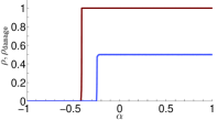
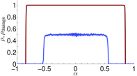
Figure 3.1: Empirical defect (dark red) and damage (light blue) density profiles at time $10^{5}$ for rules 22, 30, and 54.

To compare the damage and defect dynamics, we will assume they initially agree, i.e., that ${\text{\tt damage}}_{0}=\delta_{0}=\Delta_{0}$ is a finite set. The dynamics $\delta_{t}$ of defect sites only tracks one-site perturbations of $\xi_{t}$, while ${\text{\tt damage}}_{t}$ performs simultaneous changes at all perturbed sites, so there might be significant difference between the two. Three examples of density and damage profiles started from a uniform product measure are in Fig. 3.1. Observe that for Rule 22 $\rho_{\text{\tt damage}}<\rho$ but $W\subsetneqq W_{\text{\tt damage}}$; in fact $W_{\text{\tt damage}}$ has edges at about $\pm 0.77$ [Gra2], while those of $W$ lag behind by about $0.025$. Another CA for which $\delta_{t}$ similarly lags behind ${\text{\tt damage}}_{t}$ is Rule 122, but in this instance the empirical evidence indicates that the difference disappears in the limit, as $W=W_{\text{\tt damage}}=[-1,1]$. On the other hand, two chaotic examples for which $W_{\text{\tt damage}}\subsetneqq W$ are also included in Fig. 3.1. We also remark that, for additive rules such as Rule 150, $W_{\text{\tt damage}}$ does not exist due to the fractal evolution of ${\text{\tt damage}}_{t}$, which is, for the same reason, much smaller than $\delta_{t}$ for most (but not all) times $t$.

Assume now that the initial state is more general, a product measure with density $p$. For elementary CA, we address the dependence of defect accumulation dynamics on $p$ in Section 4.5. In this setting, rules with significant variation in $p$ coincide with rules in which $W$ is an interval of positive length while $W_{\text{\tt damage}}$ is at most a singleton for all $p\in(0,1)$. (See Proposition 4.6 for a formal proof in case of Rule 38.) This equivalence is interesting enough for a thorough theoretical development, which we do not attempt here. Instead, we provide a definition and a non-rigorous explanation next.

We call a one-dimensional CA trajectory $\xi_{t}$ striped (resp., degenerate) if there exist a translation number $v_{0}\in{\mathbb{Z}}$, a delay time $t_{0}\geq 1$, an initial time $t_{i}\geq 0$, and an $\epsilon>0$ so that $\xi_{t+t_{0}}(x)=\xi_{t}(x-v_{0})$ (resp., $\xi_{t}(x+1)=\xi_{t}(x)$) for $t\geq t_{i}$ and $x\in[(\inf{\mathcal{N}}-\epsilon)t,(\sup{\mathcal{N}}+\epsilon)t]$.

A stripes CA is one whose trajectory is almost surely striped and non-degenerate for any initial product measure with density $p\in(p_{1},p_{2})$. Here, $(p_{1},p_{2})$ is a nonempty interval of densities which is, when unspecified, assumed to be $(0,1)$. For such CA, the statistical properties of the invariant striped state typically depend on $p$. Consequently, if a stripes CA is expansive, then we expect that the Lyapunov profile also varies with $p$. On the other hand, it is easy to see that if $\xi_{t}$ and its perturbation $(\xi_{t}+{\text{\tt damage}}_{t})\operatorname{mod}2$ are both striped, ${\text{\tt damage}}_{t}$ remains bounded. For product measures, a striped trajectory typically results from transient structures that are eroded away at exponential rate, and this property cannot be changed by a finite perturbation. For such trajectories, $W_{\text{\tt damage}}$ is at most a singleton. Therefore, the equivalence discussed above is a consequence of the fact that all expansive elementary CA started from product measures are either attracted to a chaotic or complex state for any density $p\in(0,1)$, or are stripes CA. We now discuss two examples with ${\mathcal{N}}=\{0,\pm 1,\pm 2\}$ that show that there are other possibilities for general CA.

The first CA is simple: the update rule is $abcde\mapsto 1$ if and only if $abcde$ includes $010$ as a substring. The resulting global rule $\Phi$ satisfies $\Phi^{2}=0$, as for any $\xi_{0}$ there are no isolated $1$s at time $t=1$ and then no $1$s at all at time $t=2$. This is a degenerate case, and indeed $W_{\text{\tt damage}}=\emptyset$, but $W=[-1,1]$ and $\lambda_{\infty}=\log 3$ for all initial states (as the defect dynamics coincides with that for Rule 150 from time $1$ on). In particular, there is no dependence on $p$ but very large discrepancy between $W$ and $W_{\text{\tt damage}}$.

Our second counterexample is a “particle” CA that conserves the density of $1$s. A $1$ at $x$ makes a jump to $x+2$ if the states in $[x,x+2]$ are $100$ and it makes a jump to $x-1$ if the states at $[x-2,x+1]$ are $1011$. Simulations make it clear that trajectories from random initializations are not striped, and that this rule is marginal for small $p$ (with $W=\{2\}$) and expansive for large $p$, with a phase transition somewhere between $0.2$ and $0.3$. Moreover, $W_{\text{\tt damage}}=W$ at all $p\in(0,1)$, by contrast to the dramatic dependence on $p$.

4 Elementary cellular automata

In this section we investigate the defect accumulation dynamics for the elementary CA, the one-dimensional rules with ${\mathcal{N}}=\{-1,0,1\}$. The initial configuration $\xi_{0}$ will be the default uniform product measure, except in Section 4.5, where we discuss product measures with other constant densities. In these circumstances, the defect dynamics remains essentially equivalent if the roles of the two states are switched, or if the rule is replaced by its left-right reflection. This leaves us with 88 equivalence classes represented by 88 “minimal” CA [Vic2], which we proceed to analyze. The update functions for rules featured in our rigorous arguments (here or in Section 6.2) are given in Table 4.1.

Table 4.1: Update functions for some elementary CA.

Rule	$000$	$001$	$010$	$011$	$100$	$101$	$110$	$111$
22	$0$	$1$	$1$	$0$	$1$	$0$	$0$	$0$
27	$1$	$1$	$0$	$1$	$1$	$0$	$0$	$0$
38	$0$	$1$	$1$	$0$	$0$	$1$	$0$	$0$
110	$0$	$1$	$1$	$1$	$0$	$1$	$1$	$0$
152	$0$	$0$	$0$	$1$	$1$	$0$	$0$	$1$

Many of the $88$ rules are quite transparent and a simple worst case analysis as elucidated in our next two theorems yields a rigorous result. The first theorem gives the condition under which defect growth is restricted.

Theorem 4.1.

Assume that there exist a string $B\in\{0,1\}^{b}$, $b>0$, a time $t_{B}$, and a number $v_{B}$ with the following property. Any pair $(\xi_{0},\delta_{0})$, such that $\xi_{0}$ equals $B$ on $[0,b-1]$ and $\delta_{0}$ is 1 exactly on the complement $[0,b-1]^{c}$, yields $\xi_{t_{B}}|_{[v_{B},v_{B}+b-1]}=B$ and $\delta_{t_{B}}|_{[v_{B},v_{B}+b-1]}\equiv 0$. Then, if $\xi_{0}$ is any translation invariant product measure with ${\mathbb{P}\/}(\xi_{0}(x)=1)\in(0,1)$, $L_{\infty}$ equals $-\infty$ off $\{v_{B}/t_{B}\}$. In particular, with such an initialization, the defect accumulation dynamics is not expansive.

Proof.

Assume a finite $\delta_{0}$. A translate of $B^{\prime}$ consisting of $t_{B}$ contiguous copies of $B$ (almost surely) exists somewhere to the right of the support of $\delta_{0}$. Suppose that, at some time $t$, an interval $[x,x+b\cdot t_{B}-1]$ has the following two properties: all defects are to its left; and it is occupied by a translate of $B^{\prime}$. As defects cannot advance faster than by distance $1$ at each time step, and by the hypotheses, the interval $[x+v_{B},x+b\cdot t_{B}-1+v_{B}]$ has the same properties at time $t+t_{B}$. It follows that $\delta_{t}\subset(-\infty,N+t\cdot v_{B}/t_{B}]$ for all $t\geq 0$ and some a.s. finite random variable $N$. Consequently, $W\subset(-\infty,v_{B}/t_{B}]$ a.s. As this is true for any finite $\delta_{0}$, $L_{\infty}\equiv-\infty$ on $(v_{B}/t_{B},\infty)$. An analogous argument shows that the same holds for $(-\infty,v_{B}/t_{B})$ ∎

If $B$ and $t_{B}$ are fixed, the property required by Theorem 4.1, can be checked by a finite verification. Namely, to look for all possible $v_{B}$, all $2^{4t_{B}}$ possible initial configurations in $2t_{B}$ sites both to the left and to the right of $B$ are generated and then the dynamics is run to the time $t_{B}$. If it happens that $B$ occurs at two (or more) distinct intervals of $b$ sites at time $t_{B}$, then Theorem 4.1 implies the rule is collapsing.

We now state a general result in the opposite direction, i.e., we give a condition that guarantees defect expansion. Recall that $L_{{\mathcal{M}}}$ is the Lyapunov profile for the additive dynamics with neighborhood ${\mathcal{M}}$.

Theorem 4.2.

Assume that there exist a set ${\mathcal{M}}\subset{\mathbb{Z}}$ with at least two points and a time $t_{\mathcal{M}}$ with the following property: for $\delta_{0}=\mathbbm{1}(0)$ and arbitrary $\xi_{0}$, $\delta_{t_{{\mathcal{M}}}}\equiv 1$ on ${\mathcal{M}}$. Then

$$L_{\infty}(\alpha)\geq\frac{1}{t_{\mathcal{M}}}L_{{\mathcal{M}}}(t_{\mathcal{M}}\alpha).$$

In particular, the defect accumulation dynamics is expansive.

Proof.

This follows from a simple induction argument. ∎

4.1 Elementary CA with provably collapsing defect dynamics

Theorem 4.1 implies defect collapse for the $8$ rules listed in Table 4.2.

Table 4.2: The $8$ provably collapsing rules.

Rule	class	proof
0	C	trivial
8	C	$B=0$, $t_{B}=1$, $v_{B}=-1,0$
32	C	$B=0$, $t_{B}=1$, $v_{B}=\pm 1$
40	C	$B=00$, $t_{B}=1$, $v_{B}=-1,0$
128	C	$B=0$, $t_{B}=1$, $v_{B}=-1,0,1$
136	C	$B=0$, $t_{B}=1$, $v_{B}=-1,0$
160	C	$B=0$, $t_{B}=1$, $v_{B}=\pm 1$
168	C	$B=00$, $t_{B}=1$, $v_{B}=-1,0$

4.2 Elementary CA with provably marginal defect dynamics

The rules for which we are able to verify the hypotheses of Theorem 4.1 to prove marginal defect dynamics are listed in the Table LABEL:ECA-marginal. We do not provide the arguments that these cases are indeed not collapsing; these can be obtained at a glimpse from examples generated by random initial states (e.g., see Fig. 1.1 for Rule 7). The MLE directions are given by application of Theorem 4.1, while approximate MLE values are based on empirical evidence: we ran a random configuration with an interval of $10^{3}$ defects for $10^{5}$ time steps. However, as we have not attempted a rigorous determination, it is possible that rare favorable configurations result in values higher than we obtained. For example, Rule 73 seems a good candidate for this to occur.

Table 4.3: The $46$ rules with provably marginal defect accumulation dynamics.

Rule	class	proof	MLE dir.	MLE
1	M	$B=1$, $t_{B}=2$, $v_{B}=0$	$0$	$0.55$
2	M	$B=0$, $t_{B}=1$, $v_{B}=-1$	$-1$	$0$
3	M	$B=00$, $t_{B}=2$, $v_{B}=1$	$1/2$	$0.35$
4	M	$B=0$, $t_{B}=1$, $v_{B}=0$	$0$	$0$
5	M	$B=1$, $t_{B}=2$, $v_{B}=0$	$0$	$0.35$
7	M	$B=11$, $t_{B}=2$, $v_{B}=1$	$1/2$	$0.35$
10	M	$B=0$, $t_{B}=1$, $v_{B}=-1$	$-1$	$0$
12	M	$B=0$, $t_{B}=1$, $v_{B}=0$	$0$	$0$
13	M	$B=01$, $t_{B}=1$, $v_{B}=0$	$0$	$0.48$
15	M	$B=0$, $t_{B}=2$, $v_{B}=2$ (right shift w. toggle)	$1$	$0$
19	M	$B=00$, $t_{B}=2$, $v_{B}=0$	$0$	$0.35$
23	M	$B=00$, $t_{B}=2$, $v_{B}=0$	$0$	$0.69$
24	M	Prop. 4.3	$1$	$0$
27	M	Prop. 4.5	$1/2$	$0$
28	M	$B=01$, $t_{B}=1$, $v_{B}=0$	$0$	$0.48$
29	M	$B=01$, $t_{B}=1$, $v_{B}=0$	$0$	$0.35$
33	M	Prop. 4.3	$0$	$0.66$
34	M	$B=0$, $t_{B}=1$, $v_{B}=-1$	$-1$	$0$
36	M	$B=00$, $t_{B}=1$, $v_{B}=0$	$0$	$0$
42	M	$B=0$, $t_{B}=1$, $v_{B}=-1$	$-1$	$0$
44	M	$B=00$, $t_{B}=1$, $v_{B}=0$	$0$	$0.48$
46	M	Prop. 4.3	$-1$	$0$
50	M	$B=01$, $t_{B}=2$, $v_{B}=0$	$0$	$0.48$
51	M	$B=0$, $t_{B}=2$, $v_{B}=0$ (toggle)	$0$	$0$
72	M	$B=0$, $t_{B}=1$, $v_{B}=0$	$0$	$0.69$
73	M	$B=0110$, $t_{B}=1$, $v_{B}=0$	$0$	$0.91$
76	M	$B=0$, $t_{B}=1$, $v_{B}=0$	$0$	$0$
77	M	$B=01$, $t_{B}=1$, $v_{B}=0$	$0$	$0.69$
78	M	$B=10$, $t_{B}=1$, $v_{B}=0$	$0$	$0.48$
94	M	$B=101$, $t_{B}=1$, $v_{B}=0$	$0$	$0.61$
104	M	$B=00$, $t_{B}=1$, $v_{B}=0$	$0$	$0.69$
108	M	$B=00$, $t_{B}=1$, $v_{B}=0$	$0$	$0.86$
130	M	$B=0$, $t_{B}=1$, $v_{B}=-1$	$-1$	$0$
132	M	$B=0$, $t_{B}=1$, $v_{B}=0$	$0$	$0$
138	M	$B=0$, $t_{B}=1$, $v_{B}=-1$	$-1$	$0$
140	M	$B=0$, $t_{B}=1$, $v_{B}=0$	$0$	$0$
152	M	Prop. 4.4	$1$	$0$
156	M	$B=01$, $t_{B}=1$, $v_{B}=0$	$0$	$0.69$
162	M	$B=0$, $t_{B}=1$, $v_{B}=-1$	$-1$	$0$
164	M	$B=00$, $t_{B}=1$, $v_{B}=0$	$0$	$0$
170	M	$B=0$, $t_{B}=1$, $v_{B}=-1$ (left shift)	$-1$	$0$
172	M	$B=00$, $t_{B}=1$, $v_{B}=0$	$0$	$0.48$
178	M	$B=01$, $t_{B}=2$, $v_{B}=0$	$0$	$0.69$
200	M	$B=0$, $t_{B}=1$, $v_{B}=0$	$0$	$0.69$
204	M	$B=0$, $t_{B}=1$, $v_{B}=0$ (identity)	$0$	$0$
232	M	$B=00$, $t_{B}=1$, $v_{B}=0$	$0$	$0.69$

For some rules, Theorem 4.1 does not apply directly but only after a transient period; we collect the necessary properties in our next three results. We remark that agreement of the dynamics of two CA after a transient time does not necessarily imply that their defect accumulation dynamics agree.

Proposition 4.3.

The following hold for arbitrary initial states:

1. Rule 24: All $1$s are isolated at time $t=1$; thereafter, the CA evolves as Rule 2.

2. Rule 33: Every isolated $0$ at $(x,t)$, $t\geq 1$, requires two isolated $0$s at $(x\pm 1,t-1)$. If a configuration has no isolated $0$s, the CA evolves as Rule 1.

3. Rule 46: There is no isolated $1$ at time $t=1$; thereafter, the CA evolves as Rule 42.

Proof.

These are all straightforward verifications. ∎

Proposition 4.4.

Assume the CA is Rule 152. States $11$ at $(x,t)$, $(x+1,t)$, $t\geq 1$ require $111$ at $(x,t)$, $(x+1,t)$, $(x+2,t)$; if a configuration has only isolated $1$s the CA evolves as Rule 16, which is equivalent, via a left-right reflection, to Rule 2. Furthermore, if $\xi_{0}$ is the uniform product measure, then almost surely there exists an $x$ such that there is no $11$ in $[x-2+t,x+t+2]$ for all $t$. Consequently, Rule 152 is marginal.

Proof.

These are simple checks, other than the last statement. To prove the latter, let $A_{x}$ be the event that the initial configuration is $00000$ in $[x,x+4]$ and that, for every $n\geq 0$, the interval $[x+5+n,x+5+2n]$ contains at least one $0$. It suffices to show that

(4.1) $${\mathbb{P}\/}(A_{x}\text{ happens i.o.~{}for }x\geq 0)={\mathbb{P}\/}(A_{x}\text{ happens i.o.~{}for }x\leq 0)=1.$$

Let $B_{x}$ be the event that $[x,x+4]$ contains only $0$s and that the following holds for any interval $I_{x,k}=[x+5+2^{k},x+5+2^{k+1}-1]$ of length $2^{k}$: if $0\leq k\leq 4$, the entire $I_{x,k}$ is covered by $0$s; and if $k>4$, each of the four disjoint subintervals of $I_{x,k}$ of length $2^{k-4}$ contains at least one $0$. We claim that $B_{x}\subset A_{x}$. Indeed, if $2^{k}\leq n<2^{k+1}$, then the interval $[x+5+n,x+5+2n]$ has its left endpoint in $I_{x,k}$ and length at least $2^{k}+1$. Then it either covers the right half of $I_{x,k}$ or the left quarter of $I_{x,k+1}$.

Now, let

$$a={\mathbb{P}\/}(B_{0})=2^{-20}\prod_{k=5}^{\infty}\left(1-2^{-2^{k-4}}\right)^{4}>0.$$

Then ${\mathbb{P}\/}(B_{x})=a$ for every $x$. Moreover, for a large $r$, chose the largest $\ell$ so that $r\geq 5+2^{\ell}$; then

$$a\leq{\mathbb{P}\/}(B_{x}|B_{x+r})\leq\frac{a}{\prod_{k\geq\ell}\left(1-2^{-2^{k-4}}\right)^{4}}\leq a(1+c2^{-r}),$$

for some constant $c>0$. The second moment method now easily proves (4.1) with $B_{x}$ in place of $A_{x}$ and ends the proof. ∎

Proposition 4.5.

Assume the CA is Rule 27. Assume that $\xi_{0}$ and $\delta_{0}$ both vanish on $[a,b]$, where $b-a\geq 5$. Then for all even $t$, $\xi_{t}$ and $\delta_{t}$ both vanish on $[a+t/2,b+t/2-4]$. Consequently, this rule is marginal.

Proof.

We begin with a few observations. Assume that $t\geq 1$ and that the pair configuration $10$, underlined in (4.2), appears in $\xi_{t}$. Then there are two possibilities for the nearby states in $\xi_{t-1}$ (represented by the top line) and $\xi_{t}$, as depicted in (4.2). An analogous property, also given in (4.2), holds for the pair $01$.

(4.2) $$011 \quad 0010 1011 \;\;\quad 100$$

$$\phantom{0}\underline{10} \quad 1\underline{10} 0\underline{01} \;\;\quad\underline{01}1$$

It immediately follows that $1010$ is only possible in the initial state. Assume next that $0101$ occurs in $[1,4]$ in $\xi_{t}$. Then we claim that for any $k\geq 0$ and time $t-2k\geq 0$, the configuration in $[t-k,t+2k+4]$ is

(4.3) $$\text{\scalebox{3.0}[1.0]{$\square$}}\ldots\text{\scalebox{3.0}[1.0]{$\square$}}00101$$

where there are $k$ $\square$ blocks of length $3$, each containing either $001$ or $011$. We also claim that at time $t-2k-1$ the configuration at $[t-k,t+2k+5]$ must be

(4.4) $$\text{\scalebox{3.0}[1.0]{$\square$}}\ldots\text{\scalebox{3.0}[1.0]{$\square$}}101100$$

where now each of the $k$ $\square$ blocks of length $3$ contains either $100$ or $101$. Our induction hypothesis is that both (4.3–4.4) are satisfied at each $k\geq 0$. For $k=0$, this is an easy verification using (4.2). The induction step is also straightforward using the fact that the update rule satisfies $00*\mapsto 1$, $*10\mapsto 0$, and $1\!*\!1\mapsto 0$.

We now state four key facts. The first two are about the original CA and the next two about the defect percolation CA. The first fact follows from the claim above, while the remaining three are straightforward.

• As (4.3) does not contain $000$, if $\xi_{0}$ vanishes on $[x,x+2]$ in $\xi_{0}$, then the state of $\xi_{t}$ cannot contain $0101$ on the interval $[x-t,x+t/2+3]$ for any even $t\geq 0$.

• Suppose that $\xi_{0}(0)=0$ and the five state configuration of $\xi_{0}$ in $[-1,3]$ contains neither $0101$ nor $1010$. Then $\xi_{2}(1)=0$.

• If $\xi_{0}$ vanishes on $[0,1]$ and $\delta_{0}(0)=0$, then $\xi_{2}(1)=0$ and $\delta_{2}(1)=0$.

• If $\xi_{0}$ and $\delta_{0}$ both vanish on $[0,1]$, and $\xi_{0}$ is not $101$ on $[2,4]$, then $\xi_{2}$ vanishes on $[1,2]$ and $\delta_{2}(1)=0$.

The above four facts establish the claimed “non-invasion” of the interval of $0$s in the statement, and marginality easily follows. ∎

4.3 Elementary CA with expansive defect dynamics

There is overwhelming empirical evidence that the 22 rules in Table 4.4 are expansive. For nine of these cases we provide a proof: four are additive or nearly additive (rules 60, 90, 105, and 150), four more are handled by Theorem 4.2 (rules 30, 45, 54, and 57), and Rule 38 is the subject of our next result. This last rule is a stripes CA, as a disordered state self-organizes into a random configuration which is merely shifted (see Section 3 for a formal definition). With some confidence we conjecture (although we do not have a proof) that rules 6, 25, 26, 41, 57, 62, 134 and 154 are also stripes CA. In Section 4.5, we will see that these rules are also characterized by the dependence of MLE on the initial density of $1$s in $\xi_{0}$, as expected from the discussion in Section 3.

Table 4.4 gives (in most cases empirical) estimates of the MLE, its direction, defect shape $W$, and the defect density $\rho$ on $W$, which appears constant in all cases. Fig. 4.1 depicts Lyapunov profiles for Rule 30 and Rule 106, two rules that leave the uniform product measure invariant. See Section 4.5 for a discussion on Rule 62.

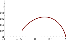
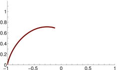
Figure 4.1: Empirical Lyapunov profiles for rules 30 and 106 at $t=10^{5}$.

Table 4.4: The $23$ expansive rules.

Rule	class	proof	MLE dir.	MLE	$W$	$\rho$
6	E	—	$-0.29$	$0.55$	$[-1,0.36]$	$0.84$
18	E	—	$0$	$0.69$	$[-1,1]$	$0.5$
22	E	—	$0$	$0.87$	$[-0.74,0.74]$	$0.86$
25	E	—	$-0.17$	$0.52$	$[-0.83,0.5]$	$1$
26	E	—	$-0.32$	$0.41$	$[-1,0.23]$	$1$
30	E	${\mathcal{M}}=\{1,3\}$, $t_{\mathcal{M}}=3$	$0.31$	$0.66$	$[-0.41,1]$	$1$
38	E	Prop. 4.6	$-0.41$	$0.54$	$[-1,0.1]$	$1$
41	E	—	$0.02$	$0.86$	$[-0.75,1]$	$0.94$
45	E	${\mathcal{M}}=\{0,2\}$, $t_{\mathcal{M}}=2$	$0.22$	$0.72$	$[-0.48,1]$	$1$
54	E	${\mathcal{M}}=\{0,\pm 1\}$, $t_{\mathcal{M}}=3$	$0$	$0.74$	$[-0.85,0.85]$	$1$
57	E	${\mathcal{M}}=\{0,\pm 1\}$, $t_{\mathcal{M}}=3$	$0$	$0.69$	$[-1,1]$	$1$
60	E	additive	$1/2$	$0.69$	$[0,1]$	$1$
62	E	—	$0$	$0.44$	$[0,0.53]$	$1$
90	E	additive	$0$	$0.69$	$[-1,1]$	$1$
105	E	additive with toggle	$0$	$1.1$	$[-1,1]$	$1$
106	E	—	$-0.26$	$0.71$	$[-1,-0.11]$	$1$
110	E	—	$-0.25$	$0.66$	$[-0.88,0.67]$	$1$
122	E	—	$0$	$0.65$	$[-1,1]$	$1$
126	E	—	$0$	$0.71$	$[-1,1]$	$1$
134	E	—	$-0.21$	$0.51$	$[-1,0.49]$	$0.81$
146	E	—	$0$	$0.69$	$[-1,1]$	$0.5$
150	E	additive	$0$	$1.1$	$[-1,1]$	$1$
154	E	—	$-0.42$	$0.48$	$[-1,0.11]$	$1$

We should also mention that it is easy to check that Rule 154 and Rule 106 are right permutative [GG5] and thus at least not collapsing, with ${\mathcal{M}}=\{-1\}$, $t_{\mathcal{M}}=1$. In fact, due to the $\limsup$ in the definition of $L$ (2.1), there are seven other rules that are provably not collapsing as a defect at the origin must generate at least one successor, although its location varies with $\xi_{0}$. These rules are 37, 41, 56, 62, 110, 134, 146, and 184.

Another remark is that the three quasi-additive rules studied by E. Jen [Jen], 18, 146 and 126, all feature annihilating dislocations that make the CA approach Rule 90. This apparently causes the Lyapunov profile to be indistinguishable from the one for Rule 90 for the first two rules (thus the MLE is $\log 2$), but not for Rule 126 whose defect dynamics differs from that for Rule 90 even in the invariant state.

Proposition 4.6.

Assume the CA is Rule 38. If $\Delta_{0}\subset[-r,r]$, then ${\text{\tt damage}}_{t}\subset[-t-r,-t+r+3]$. On the other hand, the defect accumulation dynamics is expansive; in fact, $L_{\infty}$ is strictly positive on $(-1,\alpha_{r}]$, where $\alpha_{r}=308/2977$ and $W=[-1,\alpha_{r}]$.

Proof.

First observe (by a simple verification) that there is no $0101$ in $\xi_{t}$, for $t\geq 1$, and then no $111$ for $t\geq 2$. We will assume $t\geq 2$ from now on. Any $0100$ (resp. $0110$) starting at $x$ at time $t\geq 2$ generates $0110$ (resp. $0100$) starting at $x-1$ at time $t+1$. Thus the entire configuration $\xi_{t+2}$ is obtained by shifting $\xi_{t}$ to the left by $2$. This proves the first claim.

As the rule has no stable update, a full interval of defects can only be eroded at speed one from the edges. Assume (without loss of generality) that the left edge of an interval of defects of length at least $3$ is on an infinite diagonal (of slope $1$) of $1$s. Then the boundary arrangement (with a defect site $(x,t)$ underlined) is one of these four: $00\underline{1}0$, $10\underline{1}0$, $00\underline{1}1$, $10\underline{1}1$. In all cases the defect at $(x,t)$ branches into two defects, one at $(x,t+1)$ and one at $(x-1,t+1)$. Thus the left edge of the defect interval advances at light speed.

There are six possible arrangements at the right edge at $(x,t)$ (underlined); we write $\downarrow$ when the edge stays at $x$ at time $t+1$ and $\searrow$ when it moves to $x+1$ (that is, when the defect branches into two):

$$0\underline{0}00\,\downarrow\quad 0\underline{0}01\,\downarrow\quad 0\underline{0}10\,\searrow\quad 0\underline{0}11\,\downarrow\quad 0\underline{1}00\,\downarrow\quad 1\underline{1}00\,\downarrow$$

Thus the right edge never retreats and advances when in contact with the diagonal in one of the two “phases.”

To be more precise, we first provide a convenient Markovian description of $\xi_{2}$. Consider the set $H$ of $24$ pairs $(s,a)$, where $s$ is a binary strings of length $4$ that does not contain $111$ or $0101$, and $a$ is either $0$ or $1$. Call $x\in{\mathbb{Z}}$ in a state $(s,a)$ if the string $s$ ends at $x$ and $x\in a+2{\mathbb{Z}}$. As sites at distance $5$ or more have independent $\xi_{2}$-state, this is a Markov chain. Define the following subsets of $H$,

(4.5) $$H_{1}=\{(0011,1),(1011,1),(0010,0),(1010,0)\}$$

$$H_{2}=\{(0011,0),(1011,0),(0010,1),(1010,1)\}$$

Start in (say) the state $(0011,0)$ at $x=0$, and consider the successive states of the chain given by positive integers. Define $\tau_{0}=0$ and then let $\tau_{k}$, $k=1,2,\ldots$ be the number of steps after $\tau_{k-1}$ needed to enter $H_{1}$ (even $k$) or $H_{2}$ (odd $k$). For example, if $\xi_{2}$ on ${\mathbb{Z}}_{+}$ happens to be $101100110010\ldots$, then $\tau_{1}=3$ and $\tau_{2}=8$.

By the preceding part of the proof, the right edge of $\delta_{t}$ is at $n$ at time $\sum_{i=1}^{n}\tau_{i}-n$. By symmetry, almost surely,

$$\lim_{n\to\infty}\frac{1}{n}\sum_{i=1}^{n}\tau_{i}=\frac{\sum_{h\in H_{1}}\pi(h){\mathbb{E}\/}T(h,H_{2})}{\sum_{h\in H_{1}}\pi(h)}.$$

Here, $\pi$ is the invariant measure and ${\mathbb{E}\/}T(h,H_{2})$ is the expected time to reach $H_{2}$ from $h$, both readily computable by a matrix computation to get the limit $3285/308$. The right edge of $W$ then is

$$\lim_{n\to\infty}\frac{n}{\sum_{i=1}^{n}\tau_{i}-n}=\alpha_{r}.$$

Finally, we prove the claim that $L_{\infty}>0$ on $(-1,\alpha_{r}]$. For this, it is sufficient to show that

(4.6) $$L_{\infty}(\alpha_{r})=\alpha_{r}\log 2$$

as then, by just considering defects that accumulate on the path that first moves on the right edge and then on a leftward diagonal of $1$s,

$$L_{\infty}(\alpha)\geq\frac{\alpha_{r}\log 2}{\alpha_{r}+1}(\alpha+1)$$

on $[-1,\alpha_{c}]$. To prove (4.6), observe first that the only Rule 38 update that is sensitive to a change of both left and center input is $010\mapsto 1$. The number of paths at the right edge thus goes up by a factor of $2$ precisely when the rightmost defect is on the middle $1$ of $010$. The number of times this happens is exactly the number of states in $H_{1}$ (resp. in $H_{2}$) in $[\tau_{k}+1,\tau_{k+1}]$ for odd $k$ (resp. even $k$). The expected number of such states is $1$, by elementary Markov chain theory, and so the number of paths at the right edge at time $\sum_{i=1}^{n}\tau_{i}-n$ is $2^{N_{n}}$ where $N_{n}/n\to 1$ a.s. as $n\to\infty$. The claimed equality (4.6) follows. ∎

While Proposition 4.6 determines its support, a full characterization of the Lyapunov profile in cases such as Rule 38 is closely related to quenched large deviations for random walks in a random environment (see e.g. [Yil]). A computationally viable variational technique is beyond current methods (which in particular require nondegeneracy conditions that Rule 38 walks fail to satisfy) and seems a very interesting open problem.

4.4 Classification of the remaining elementary CA

The remaining $11$ rules are gathered in Table 4.5, with conjectured class and other empirical information.

Table 4.5: The $11$ remaining rules.

Rule	class	notes	MLE dir.	MLE
9	M	long transient period	$1$	$0$
11	M	medium transient period	$1$	$0$
14	C	gliders erode defects	—	—
35	M	medium transient period	$1/2$	$0$
37	M	medium transient period	$0$	$0.35$
43	C	gliders erode defects	—	—
56	M	medium transient period	$1$	$0$
58	M	long transient period	$-1$	$0$
74	M	medium transient period	$-1$	$0$
142	C	gliders erode defects	—	—
184	M	defects percolate when gliders collide	$0$	$0$

All these dynamics feature a relatively simple invariant state, an ether, which supports a variety of annihilating gliders. A detailed quantitative analysis of the glider dynamics necessary for the proof may be possible in some cases (for some results in this direction, see [BF] for Rule 184, and density computations of the three collapsing rules in Section 4.5), but is beyond the scope of this paper. However, we observe that the glider configuration for seven of these CA appears to stabilize at an exponential rate (hence the reference to the “transient period”), while Rule 184 and the three collapsing rules feature recurrent glider collisions that drive their density to zero much more slowly, at the rate $t^{-1/2}$ (by the argument in [DS] for a similar dynamics).

4.5 Dependence of defect accumulation on initial density for elementary CA

We now turn our attention to how the defect accumulation depends on the density of $1$s in the initial CA configuration. We will assume that $\xi_{0}$ is the product measure with constant $p={\mathbb{P}\/}(\xi_{0}(x)=1)\in(0,1)$, and mostly study how MLE varies with $p$. Our next result greatly reduces the rules we need to consider.

Theorem 4.7.

All rules in Table LABEL:ECA-marginal are marginal for all $p\in(0,1)$, and their Lyapunov profile $L_{\infty}$ does not depend on $p$.

Proof.

The proof of the equivalence property for Rule 152 in Proposition 4.4 is easily adapted. The remainder follows from the fact than any finite configuration occurs infinitely often in any nontrivial uniform product measure. ∎

With one exception, we expect that Theorem 4.7 holds also for the marginal rules in Table 4.5. The special case is Rule 184, which does not have a transient defect dynamics when $p=1/2$ [BF], but the transience does hold for other $p$. Furthermore, the defect dynamics is marginal for all $p$, and the MLE does not depend on $p$, but its direction does: it is $1$ for $p<1/2$, $0$ for $p=1/2$ and $-1$ for $p>1/2$.

The three collapsing rules in Table 4.5 are at first quite mysterious and computer simulations do not offer conclusive evidence even on the classification of the defect dynamics near $p=1/2$. Therefore, we need to to take a closer look at gliders for these three CA. As the analysis for Rule 142 is almost exactly the same as for Rule 14, we will only discuss the latter and Rule 43 in detail. For both of these, the ether is the configuration $(0011)^{\infty}$, which gets translated to the left by $1$ every time step. There are two kinds of gliders, leftward- and rightward-moving ones, at sites with local configurations as given in Table 4.6 (with a glider site and direction indicated by the arrow). As we see from this table, one or the other type of gliders “wins” when $p\neq 1/2$. However, for the advantage to be detectable empirically, the array size would have to be on the order of at least $1/(2p-1)^{4}$, too impractical when $p=0.51$, say. From simulations we conclude that glider imbalance leads to marginal dynamics with the MLE equal to $0$ in both cases and the MLE direction either $-1$ (for Rule 14) or $1$ (for Rule 43). When $p=1/2$, the glider dynamics has the same behavior as in Rule 184 (at the same $p$), but by contrast the defects are not able to percolate through all collisions, which causes the collapse in the case of a uniform product initialization. These three rules thus do exhibit dramatic variation with $p$, albeit of a rather degenerate kind, as $\lambda_{\infty}=0$ except at a single exceptional density $p=1/2$ where $\lambda_{\infty}=-\infty$ .

Table 4.6: Gliders in rules 14 and 43 and information about their initial probabilities.

Rule	leftward glider sites	rightward glider sites	${\mathbb{P}\/}(\leftarrow)-{\mathbb{P}\/}(\rightarrow)$	${\mathbb{P}\/}(\leftarrow)$ when $p=1/2$
14	$0\!\overleftarrow{0}\!0$, $111\!\overleftarrow{1}$, $111\!\overleftarrow{0}\!0$	$0\!\overrightarrow{1}\!0$, $01\!\overrightarrow{0}\!1$, $011\!\overrightarrow{0}\!1$	$(2p-1)^{2}$	$7/32$
43	$0\!\overleftarrow{1}\!0$, $1\!\overleftarrow{0}\!1$	$0\!\overrightarrow{0}\!0$, $1\!\overrightarrow{1}\!1$	$-(2p-1)^{2}$	$1/4$

It remains to address the rules in Table 4.4. The $14$ rules that are not stripes CA are attracted to the same invariant state independent of $p$; that state is chaotic except for Rule 110 that possibly slowly converges [LN] to the periodic state with the MLE around $0.65$ discussed in Section 6.2.3. As a result, the Lyapunov profiles, and therefore the MLE, for these $14$ rules exhibit no significant variation with $p$. Next, we present evidence that the nine stripes rules, while they remain expansive, do have detectable dependence of the MLE $\lambda_{\infty}$ on $p$.

Table 4.7: Dependence of the MLE on $p\in(0,1)$ for expansive stripes CA.

Rule	min. MLE	max. MLE
6	$0.54$ at $p=0.4$	$0.69$ at $p=1-$
25	$0.35$ at $p=0+,1-$	$0.52$ for $p\in(0.4.0.6)$
26	$0.41$ at $0.37$	$0.59$ at $p=0+,1-$
38	$0.54$ at $0.5$	$0.69$ at $p=0+,1-$
41	$0.86$ for $p\in(0.15,0.85)$	$0.89$ at $p=0+,1-$
57	$0.693$ for $p=0.5$	$0.706$ at $p=0.25,0.75$
62	$0.44$ for $p\in(0.08,0.92)$	$0.47$ at $p=0+,1-$
134	$0.45$ at $p=1-$	$0.68$ at $p=0+$
154	$0.43$ at $p=0.22$	$0.69$ at $p=1-$

The nature of this dependence differs significantly among the nine expansive stripes rules and is summarized in Table 4.7. Most approximations are based on computations up to time $t=2\cdot 10^{4}$ for $99$ equally spaced densities in $(0,1)$. We use $t=10^{5}$ for the more subtle rules 57 and 62, which are discussed in greater detail below. Except for these two rules, we observe a greater MLE variability than reported in [BRR], which restricts the range of $p$, and, as reviewed in the Introduction, has a related but different definition of MLE $\lambda_{\infty}$. However, in some cases $\lambda_{\infty}$ is indistinguishable from a constant on an interval, as indicated in Table 4.7. We illustrate the density dependence by giving more details for Rule 134 (see Fig. 4.2): this rule generates the profile that spreads out with increasing $p$, as its peak decreases and its support widens.

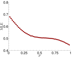
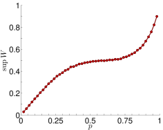
Figure 4.2: Dependence on density $p$ for Rule 134: the MLE (left) and the right edge of $W$ are graphed vs. $p$. (The left edge of $W$ stays at $-1$.)

We conclude this section with an empirical analysis of rules 57 and 62. Like for the other seven stripes rules, it is (empirically) clear that for these two $W_{\text{\tt damage}}$ is (a.s.) at most a singleton for all $p$. Unlike the others, however, they at first appear to exhibit no density dependence of MLE on $p$. This necessitates a closer inspection, and we begin with Rule 62.

As is common for stripes CA, Rule 62 dynamics undergoes a transient phase until (in this case vertical) stripes dominate. This phase is quite long-lasting, and is characterized by the annihilation of diagonal gliders, which are temporarily able to block the expansion of defects. See Fig. 4.3 for a sample evolution and the resulting Lyapunov profile.

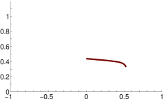
Figure 4.3: Evolution of defect percolation CA up to time $100$ and the empirical Lyapunov profile at time $10^{5}$ for Rule 62.

It turns out that the only detectable variation of the MLE and its direction occurs near $p=0$ and $p=1$. In fact, there seems to be an intriguing phase transition near $p=0.08$ that is marked by the sharp turn of MLE curve and the sudden passage of the MLE direction to $0$. See Fig. 4.4.

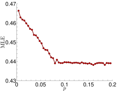
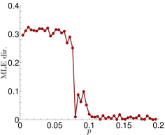
Figure 4.4: Dependence on density $p$ near $p=0$ for Rule 62: the MLE (left) and its direction are graphed vs. $p$. These graphs are based on comptations up to $t=10^{5}$.

Finally, Rule 57 is another case with pairwise annihilating gliders, which are rightward-moving pairs of $0$s and leftward-moving pairs of $1$s on a checkerboard ether. This rule is invariant under a symmetry transformation: if one switches the roles of two states, and then applies the left-right reflection, one obtains the same rule. As a consequence, temporarily using the superscript to indicate the dependence on $p$, $L^{p}_{\infty}(\alpha)=L^{1-p}_{\infty}(1-\alpha)$ and $\lambda^{p}_{\infty}=\lambda^{1-p}_{\infty}$. It is therefore enough to consider $p\in(0,1/2)$. On this interval, Rule 57 is a stripes rule, with the rightward gliders dominating. At $p=1/2$, this rule cannot be striped, as $\xi_{t}$ equals its reflection in distribution and thus neither of the two gliders can win. See Fig. 4.5 for the empirical results.

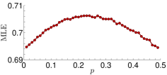
Figure 4.5: Dependence on density $p\in(0,1/2)$ for Rule 57: the MLE (left) and the left edge of $W$ are graphed vs. $p$ (the right edge stays at $1$). These are computed at $t=10^{5}$.

5 Two-dimensional cellular automata

While the theoretical set-up is similar, a two-dimensional geometry is much less restrictive than a one-dimensional one, making rigorous theory more demanding and in need of further development. We restrict our attention to totalistic rules with a von Neumann or Moore neighborhood. The one simple rigorous result we provide next identifies $8$ of the $2^{6}=64$ of the former rules, and $32$ of the $2^{10}=1024$ of the latter rules, as collapsing. The nomenclature we use is similar to the one in [Vic1]: the rule is identified by the neighborhood, and the name Tot followed by the list of occupation numbers, that is, the neighborhood counts that update to $1$. For example, Moore neighborhood Tot 1 updates $x$ to $1$ precisely when there is a single $1$ among the $9$ neighbors of $x$.

Proposition 5.1.

Assume that $\xi_{0}$ is a product measure with density $p\in(0,1)$. For Moore neighborhood, any totalistic rule for which $4,\ldots 9$ are all among the occupation numbers is collapsing. The same holds for any von Neumann rule whose occupation numbers include all of $2,\ldots,5$. Consequently, Moore (resp. von Neumann) rules that have none of $0,\ldots 5$ (resp. none of $0,\ldots,3$) among occupation numbers are also collapsing.

Proof.

Assume we have a von Neumann rule in which any site $x$ updates into state $1$ by contact with $2$ or more $1$s. The proof in the Moore case is similar, and the last two statements are proved by switching the roles of $0$s and $1$s. Call an $L\times L$ square good if the configuration within the square is such that no matter what the configuration outside the square is, the rule completely fills the square by $1$s in time $L^{2}$. By the result in [Sch], for $L$ large enough (in fact, of size $\exp(cp^{-2})$, for some constant $c$), a fixed $L\times L$ square is good with probability at least $0.9$, Note also that once such a square is filled by $1$s and free of defects, no defect can ever enter it.

Now tile ${\mathbb{Z}}^{2}$ with $L\times L$ squares. As the critical site percolation probability on ${\mathbb{Z}}^{2}$ is smaller than $0.9$, by time $L^{2}$ the good squares confine all defects into a finite set. Then that finite set is completely covered by $1$s in a finite (random) time and then the defects must all die as $11111\mapsto$ 1 is a stable update. ∎

(a)

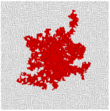
(b)

(c)

Figure 5.1: Snapshots of two-dimensional evolution of defect percolation CA: (a) von Neumann Tot 245, (b) von Neumann Tot 125, and (c) Moore Tot 1.

Needless to say, we have good empirical evidence that many more of these rules are collapsing. Possibly the most interesting cases are von Neumann Tot 245 and Moore Tot 46789 rules, both famously known as the Vishniac twist [Vic1, TM]. In these rules, the defects can survive only on the border between $0$s and $1$s, and those borders anneal away, i.e., shrink and disappear due to a process resembling surface tension. This is however a slow evolution during which the set of defect sites self-organizes into long “noodles,” as in Fig. 1(a), which features the von Neumann case.

Among the notable apparently marginal rules, we mention the “cauliflower” von Neumann rule Tot 125, in which defect sites do spread while the state is close enough to the uniform product measure, but eventually the CA reaches a state that stops further defect growth; see Fig. 1(b).

Chaotic rules are very common among totalistic ones, thus expansive defects accumulation dynamics also abound. A typical example is Moore Tot 1, whose defect percolation CA is illustrated in Fig. 1(c), while its empirical Lyapunov profile (at time $t=300$) is depicted in Fig. 5.2. We estimate its MLE to be about $1.24$.

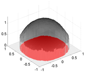
Figure 5.2: Approximation to Lyapunov profile $L$ for Tot 1. The “chiseled” boundary indicates drop to $-\infty$ and the red “shadow” approximates $\{L>-\infty\}=W$.

6 Periodic initial states

A configuration $\eta\in S^{{\mathbb{Z}}^{d}}$ is doubly periodic for a CA with global map $\Phi$ if there exist

• a number $\pi\geq 1$ so that $\Phi^{\pi}(\eta)=\eta$; and

• a number $\sigma\geq 1$ so that, for every $x$, $\eta(x)=\eta(x\operatorname{mod}\sigma)$, where $x\operatorname{mod}\sigma$ reduces every coordinate of $x$ modulo $\sigma$.

We assume that $\pi$ and $\sigma$ are the smallest possible and refer to them respectively as the temporal and spatial period. When $d=1$, it is convenient to also introduce a shift period $\pi_{0}\geq 1$, the smallest time at which there exists a shift $\sigma_{0}\in\{0,\ldots,\sigma-1\}$ such that the CA shifts $\eta$ to the right by $\sigma_{0}$ in $\pi_{0}$ steps: $(\Phi^{\pi_{0}}\eta)(x)=\eta(x-\sigma_{0})$ for all $x$. Note that $\pi_{0}$ divides $\pi$. In this section, we will assume that a doubly periodic configuration $\eta$ is the initial state $\xi_{0}$ for the CA dynamics. We often specify a periodic configuration $\eta$ by a tile, that is a configuration in $S^{[0,\sigma-1]^{d}}$ that gives $\eta$ on $[0,\sigma-1]^{d}$.

One complication in the analysis of periodic orbits is caused by reducibility. To each $\eta$ we associate the reduced kernel

$$K:{\mathbb{Z}}_{\sigma}^{d}\times{\mathbb{Z}}_{\sigma}^{d}\to\{0,1\},$$

which has $K(a,b)=1$ exactly when the defect percolation dynamics starting from $\mathbbm{1}(a)$ results in $\delta_{\pi}(x)=1$ for some $x=b\operatorname{mod}\sigma$. We call $\eta$ irreducible if $K$ is irreducible. Clearly, we may check irreducibility at time $\pi_{0}$; more on this later.

The doubly periodic configuration $\eta$ is strongly irreducible if there exists an $a\in{\mathbb{Z}}^{d}$ such that, for every $x_{0}\in{\mathbb{Z}}^{d}$, and $\delta_{0}=\mathbbm{1}(x_{0})$,

$$\cup_{t}\{x:\delta(x+ta)=1\}={\mathbb{Z}}^{d}.$$

If $\eta$ is irreducible but not strongly irreducible, then the set of points in $\{\delta_{t}=1\}$ is included in a periodic space-time lattice.

6.1 Defect shapes and density profiles

Without loss of generality we assume in this section that $\eta$ is strongly irreducible and $a=0$. In our examples, we will commonly have strong irreducibility if we neglect the sites with stable updates. We call such cases essentially strongly irreducible. We will assume that the initial set of defects $\delta_{0}$ is a $\sigma\times\sigma$ square, to prevent their accidental death. In the essentially strongly irreducible cases, the density profile $\rho$ is constant on $W$ (and of course vanishes off $W$).

For the next theorem, we let $\mathcal{S}^{d-1}\subset{\mathbb{R}}^{d}$ be the set of unit vectors, that is, the set of directions in $d$ dimensions. The half space in direction $u$ is defined by

$$H_{u}^{-}=\{x\in{\mathbb{R}}^{d}:\langle x,u\rangle\leq 0\}.$$

Theorem 6.1.

For any unit vector $u\in\mathcal{S}^{d-1}$, there exists a number $w(u)\geq 0$ so that, if $\delta_{0}=H_{u}^{-}\cap{\mathbb{Z}}^{d}$,

$$t^{-1}\delta_{t}\to w(u)u+H_{u}^{-}$$

as $t\to\infty$, in Hausdorff metric. Moreover, if we form the set

$$K_{1/w}=\bigcup_{u\in\mathcal{S}^{d-1}}\{\alpha u:0\leq\alpha\leq 1/w(u)\},$$

then the limiting shape is given by the polar transform of $K_{1/w}$,

$$W=K_{1/w}^{*}=\{x\in{\mathbb{R}}^{d}:\langle x,u\rangle\leq w(u)\}.$$

We refer to $w(u)$ as a half-space velocity [GG1, GG3, Wil]. In mathematical models of crystallography, $K_{1/w}$ is sometimes called the Frank diagram [Gig]. In our case, as can be seen from the proof, $K_{1/w}$ is a convex polygon. In $d=2$ its vertices can only be in the directions orthogonal to lines through two points of the Minkowski sum of $\pi$ copies of ${\mathcal{N}}$, i.e., $\{x_{1}+\ldots+x_{\pi}:x_{1},\ldots,x_{\pi}\in{\mathcal{N}}\}$.

Proof.

For simplicity of notation, we assume $\pi=1$; the proof is easily adapted to general $\pi$.

Interpret a subset of $S\subset{\mathbb{Z}}^{d}$ as a $\sigma^{d}$-tuple of subsets $(S_{a}:a\in{\mathbb{Z}}_{\sigma}^{d})$, where $S_{a}=S\cap(a+\sigma{\mathbb{Z}}^{d})$. Denote the set of these tuples by $\Sigma$. Using one of these tuples as the $\delta_{0}$, $\delta_{\pi}$ may be interpreted as a map $\Psi:\Sigma\to\Sigma$. Let $\widetilde{\Sigma}$ be the set of all $\sigma^{d}$-tuples of subsets of ${\mathbb{R}}^{d}$. We define the map $\widetilde{\Psi}:\widetilde{\Sigma}\to\widetilde{\Sigma}$ as follows. The image of $(\widetilde{S}_{a}:a\in{\mathbb{Z}}_{\sigma}^{d})$ is the vector of sets $(\widetilde{T}_{b}:b\in{\mathbb{Z}}_{\sigma}^{d})$ such that

(6.1) $$\widetilde{T}_{b}=\{x\in{\mathbb{R}}^{d}:0\in\Psi((\widetilde{S}_{a}-x)\cap(a+\sigma{\mathbb{Z}}^{d}):a\in{\mathbb{Z}}_{\sigma}^{d})_{b}\}.$$

In words, at each $x$, the occupation of the set at coordinate $b$ is decided by translating ${\mathbb{Z}}^{d}$ so that the $b$th lattice covers $x$, intersecting all sets with this translation, and then applying the discrete rule. It immediately follows from (6.1) that the discrete and continuous rules are conjugate:

(6.2) $$\Psi(\widetilde{S}_{a}\cap(a+\sigma{\mathbb{Z}}^{d}):a\in{\mathbb{Z}}_{\sigma}^{d})=(\widetilde{\Psi}(\widetilde{S}_{a}:a\in{\mathbb{Z}}_{\sigma}^{d})_{b}\cap(b+\sigma{\mathbb{Z}}^{d}):b\in{\mathbb{Z}}_{\sigma}^{d}).$$

The continuous rule is useful because of its translation invariance when applied to half-spaces. To formulate this property, fix a direction $u\in\mathcal{S}^{d-1}$ and a vector $(\alpha_{a}^{0}:a\in{\mathbb{Z}}_{\sigma}^{d})$. Then, there exists a vector $(\alpha_{a}^{1}:a\in{\mathbb{Z}}_{\sigma}^{d})$ so that

(6.3) $$\widetilde{\Psi}(\alpha_{a}^{0}u+H_{u}^{-}:a\in{\mathbb{Z}}_{\sigma}^{d})=(\alpha_{a}^{1}u+H_{u}^{-}:a\in{\mathbb{Z}}_{\sigma}^{d}).$$

Now iterate $\widetilde{\Psi}$ to get a sequence of vectors $(\alpha_{a}^{t}:a\in{\mathbb{Z}}_{\sigma}^{d})$, $t=0,1,\ldots$ Due to strong irreducibility and the discrete nature of the dynamics, there exist a number $w(u)\geq 0$ and an integer $k\geq 1$ so that, for a large enough $t$,

$$\alpha_{a}^{t+k}-\alpha_{a}^{t}=kw(u),$$

for every $a$. Due to monotonicity, $w(u)$ is independent of the initial vector $(\alpha_{a}^{0})$. This proves the existence of the half-space velocities. Now the theorem follows from methods from [Wil, GG1, GG3]. Observe also that $\tilde{\Psi}$ is set-additive, that is, for any $\widetilde{S}_{a},\widetilde{S}_{a}^{\prime}\subset{\mathbb{R}}^{d}$,

$$\widetilde{\Psi}(\widetilde{S}_{a}\cup\widetilde{S}_{a}^{\prime}:a\in{\mathbb{Z}}_{\sigma}^{d})=\widetilde{\Psi}(\widetilde{S}_{a}:a\in{\mathbb{Z}}_{\sigma}^{d})\cup\widetilde{\Psi}(\widetilde{S}_{a}^{\prime}:a\in{\mathbb{Z}}_{\sigma}^{d}),$$

where the second union is coordinate-wise. Writing a half-space as a union of its points, this implies that $K_{1/w}=L^{*}$ and thus $K_{1/w}$ is convex. ∎

We now turn to examples. We will restrict ourselves to two-dimensional Moore neighborhood Tot $\theta$ rules (see Section 5). We start with the observation that it is quite possible that $W=\emptyset$. For example, $\eta\equiv 0$ is a fixed state (with $\sigma=\pi=1$) for Tot $\theta$ when $\theta\geq 1$ and has $W=\emptyset$ when $\theta\geq 2$.

We start with $\theta=1$. We have generated all possible doubly periodic states with $\sigma\leq 4$. There are 12 of them (modulo symmetries of the lattice ${\mathbb{Z}}^{2}$) and none have $W=\emptyset$, although in four cases the interior of $W$ is empty. We provide two examples:

• tile $\begin{matrix}0000\\ 0000\\ 0011\\ 0011\end{matrix}$, $\pi=2$, first quarter vertices of $W$ $(2/3,0)$, $(2/5,2/5)$, $(0,2/3)$, and the defect density profile $\rho|_{W}\equiv 3/4$ on $W$ (Fig. 2(a));

• tile $\begin{matrix}0000\\ 0011\\ 0000\\ 1100\end{matrix}$, $W=[-2/3,2/3]\times\{0\}$, which has empty interior, thus $\rho\equiv 0$ (Fig. 2(b)).

For the first of these, Fig. 6.1 illustrates the relationship between the Frank diagram (the larger outline with first quarter vertices $(1,2/3)$, $(2/3,1)$, and the shape described in Theorem 6.1.

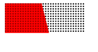
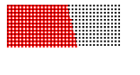
Figure 6.1: The shape characterization for our first Tot 1 example in the text. Left: propagation of the half-plane with boundary slope $-4$, depicted at times $t=0,6,12$. The configuration at $t=12$ is a horizontal translation by $4$ of the one at $t=6$, which results in the advancement by $4$ every $6$ time steps. Right: defect shape from the Frank diagram.

When $\theta=3$ there are 24 doubly periodic states with $\sigma=4$, of which we selected a nonsymmetric shape:

• tile $\begin{matrix}0000\\ 0001\\ 0010\\ 1001\end{matrix}$, with $\pi=6$, eleven vertices $(\pm 2/3,-1)$, $(8/9,-8/9)$, $(1,\pm 2/3)$, $(\pm 2/3,1)$, $(-8/9,8/9)$, $(-1,2/3)$, $(-1,-1/3)$, $(-8/9,-2/3)$, and $\rho|_{W}\equiv 5/6$ (Fig. 2(c)).

Our final example has $\theta=7$,

• tile $\begin{matrix}0111\\ 1011\\ 1110\\ 1101\\ \end{matrix}$ and $\pi=2$ (Fig. 2(d)). This case is clearly not essentially strongly irreducible. In fact, it is easy to check that defects on $0$s and $1$s do not communicate. On $1$s the defects spread as fast as the light cone, resulting in the defect shape $[-1,1]^{2}$. However, the spread on $0$s is considerably slower, resulting in the inner symmetric octagon with two of its vertices $(1,0)$, $(2/3,2/3)$. This octagon is not visible in the defect shape, but clearly shows up in the defect density profile $\rho$, which is $1$ on the octagon and $3/4$ on the region between the square and the octagon.

6.2 Lyapunov profiles in one dimension

Our discussion on Lyapunov profiles of doubly periodic configurations will be limited to $d=1$ for simplicity. Most of our techniques extend readily to higher dimensions.

6.2.1 Variational principle in the irreducible case

The input for the Lyapunov profile computation is the expansion graph $\mathcal{E}$ that we define first. The vertices of this directed graph are numbers in ${\mathbb{Z}}_{\sigma}=\{0,\ldots,\sigma-1\}$ and we attach to each edge $e$ of $\mathcal{E}$ a displacement label $D(e)$ and a size label $N(e)$. For an $i\in\{0,\ldots,\sigma-1\}$, assume $\Delta_{0}$ is $1$ at $i$ and $0$ otherwise. Suppose $\Delta_{\pi_{0}}$ has $n_{i}\geq 0$ nonzero values $N_{j}^{(i)}$ at $i+D_{j}^{(i)}$, $j=1,\ldots,n_{i}$; each of these values generates an edge $(i,i+D_{j}^{(i)}-\sigma_{0}\mod\sigma)$ of $\mathcal{E}$ emanating from $i$, with the displacement label $D_{j}^{(i)}$ and size label $N_{j}^{(i)}$. Note that an oriented pair of vertices $(i_{1},i_{2})$ may be joined by multiple edges with distinct displacement labels. Let $d_{T}=\sum_{i}n_{i}$ be the number of edges of $\mathcal{E}$. Assume the edges of $\mathcal{E}$ are ordered $e_{1},\ldots,e_{d_{T}}$, say lexicographically among the oriented pairs of vertices and by increasing displacement label within the same oriented pair.

Construct the $d_{T}\times d_{T}$ matrix $T$ as follows. If edges $e_{k}$ and $e_{\ell}$ connect ordered pairs $(i_{1},j_{1})$ and $(i_{2},j_{2})$ then

$$T_{k,\ell}=\begin{cases}N(e_{k})&\text{if }j_{1}=i_{2}\\ 0&\text{otherwise}\end{cases}$$

The weight matrix $W_{y}$, which depends on a real parameter $y$, is a diagonal matrix of the same size as $T$ given (using the order of edges) by

(6.4) $$W_{y}=\text{diag}(\exp(yD(e_{k})),k=1,\ldots,d_{T}).$$

The much simpler matrix is $T^{\prime}$ is a $\sigma\times\sigma$ matrix indexed by vertices of $\mathcal{E}$ with entries

$$T_{i_{1},i_{2}}^{\prime}=\sum_{e\in\mathcal{E}\text{ connects }(i_{1},i_{2})}N(e).$$

Thus the matrix $T^{\prime}$ counts defect paths that connect the $\sigma$ phases, while $T$ keeps track of their displacements as well.

The large deviation principles that determine $L$ have particularly simple variational form when $\eta$ is irreducible, and therefore both $T$ and $T^{\prime}$ are irreducible. This is the setting in the next theorem. We use the notation spr for the spectral radius of a matrix.

Theorem 6.2.

Assume that $\eta$ is irreducible. Then $L$ is proper, independent of $\Delta_{0}$, and is given as follows. Let

(6.5) $$\Lambda(y)=\log{\text{\tt spr}}(T\cdot W_{y}).$$

Then the Lyapunov profile $L$ is given by the Legendre transform of $\Lambda$ that is, by

(6.6) $$L(\alpha)=\inf_{y\in{\mathbb{R}}}(-y\alpha+\Lambda(y)).$$

Furthermore, let $\lambda_{1}={\text{\tt spr}}(T)$ be the largest eigenvalue of $T$. Then the MLE is given by

(6.7) $$\lambda=\log{\text{\tt spr}}(T^{\prime})=\log\lambda_{1}.$$

For $k=1\ldots,d_{T}$ define constants $c_{k}$ so that the $k$th diagonal element $T^{n}_{kk}$ of $T^{n}$ satisfies

(6.8) $$T^{n}_{kk}\sim c_{k}\lambda_{1}^{n}$$

as $n\to\infty$. Then the unique MLE direction equals

(6.9) $$\sum_{k=1}^{d_{T}}c_{k}D(e_{k}).$$

Proof.

Apart from (6.9), the claims follows from standard large deviation theory and Perron-Frobenius theory (see Section 3.1 in [DZ]).

To verify (6.9), we use further results on asymptotics of nonnegative matrices. By Section 5 of [FS], there exist a diagonal matrix $\Gamma=\text{diag}(\gamma_{1},\ldots,\gamma_{d_{T}})$ with all $\gamma_{i}>0$ and a stochastic matrix $P$ so that $T=\lambda_{1}\Gamma^{-1}P\Gamma$. Then

$$T_{ij}^{n}=\lambda_{1}^{n}\gamma_{i}^{-1}\gamma_{j}P_{ij}^{n}.$$

Let $\mu=(\mu_{1},\ldots,\mu_{d_{T}})$ be the probability measure that is a left eigenvector of $P$.

Assume that the initial edge is $e_{k}$ and that $D$ is $1$ on $e_{1}$ and $0$ otherwise. By linearity, this suffices. The expected proportion of the edge $e_{1}$ on a path of length $t$ chosen uniformly at random is

$$\frac{1}{t+1}\sum_{s=0}^{t}\frac{\sum_{\ell}T_{k1}^{s}T_{1\ell}^{t-s}}{\sum_{\ell}T_{k\ell}^{t}}\xrightarrow[t\to\infty]{}\frac{\sum_{\ell}\gamma_{k}^{-1}\gamma_{1}\mu_{1}\gamma_{1}^{-1}\gamma_{\ell}\mu_{\ell}}{\sum_{\ell}\gamma_{k}^{-1}\gamma_{\ell}\mu_{\ell}}=\mu_{1}$$

and

$$T_{11}^{n}\sim\mu_{1}\lambda_{1}^{n},$$

so that $c_{1}=\mu_{1}$ in (6.8). A similar computation also handles the second moment and finishes the proof. ∎

The constants $c_{k}$ can be readily obtained by linear algebra; for example, if $T$ has an invertible eigenvector matrix $V$, with the first column being the eigenvector of $\lambda_{1}$, and we let $I_{1}$ be the matrix with a $1$ at position $11$ and $0$s elsewhere, then $c_{k}=(VI_{1}V^{-1})_{kk}$.

Next, we give three examples. In Figs. 6.3 and 6.4, we compare the approximation to the defect profile at a modest finite time to the limit given by Theorem 6.2.

6.2.2 Two examples for Rule 22

For illustration we begin with perhaps the simplest nontrivial case, the fixed point $(10)^{\infty}$ for Exactly 1. Hence, $\sigma=2$ and $\pi=1$. We specify the tile to be $10$; we always assume that the leftmost state of the tile is at the origin, which specifies the states of $\mathcal{E}$. It is easy to check that a defect at $(x,t)$:

• creates 3 children located on a 1 at $(x,t+1)$ and on $0$s at $(x\pm 1,t+1)$, if $\xi_{t}(x)=1$; and

• creates 2 children on $1$s at $(x\pm 1,t+1)$, if $\xi_{t}(x)=0$.

This describes the graph $\mathcal{E}$, which has 5 edges, thus $d_{T}=5$,

$$T=\begin{bmatrix}0&0&0&1&1\\ 1&1&1&0&0\\ 0&0&0&1&1\\ 1&1&1&0&0\\ 1&1&1&0&0\\ \end{bmatrix}$$

and $D=(-1,0,1,-1,1)$. The resulting density profile, which is given in Fig. 3(a), is nonnegative on $W=[-1,1]$, vanishes at the boundary, and its MLE is about $0.941$. In fact, we can give the precise value for the MLE,

$$\lambda=\log{\text{\tt spr}}T^{\prime}=\log{\text{\tt spr}}\begin{bmatrix}1&2\\ 2&0\end{bmatrix}=\log\frac{1+\sqrt{17}}{2}.$$

For our second Exactly 1 example, consider the doubly periodic configuration given by the tile $1^{6}0^{2}$, which has $\sigma=8$, $\pi=6$, $\pi_{0}=3$ and $\sigma_{0}=4$. Now the defects at the middle two $1s$ die due to the fact that $111\mapsto 1$ is a stable update. Thus we only need to consider 6 states for our graph $\mathcal{E}$. This graph has no multiple edges, so we only need to specify the matrix $T^{\prime}$ and the displacements associated with each entry. These are given in the Table 6.1, from which we conclude that $d_{T}=22$. The resulting Lyapunov profile is given in Fig. 3(b). In this case there is a nontrivial defect density $\rho$ that equals $3/4$ on $W=[-2/3,2/3]$, $L$ equals $\log(2)/6\approx 0.116$ at $\pm 2/3$, and the MLE is about $0.638$.

Table 6.1: Specification for the graph $\mathcal{E}$ for the Exactly 1 example with tile $1^{6}0^{2}$. The states 2 and 3, which produce no children, are left out.

$i\in{\mathbb{Z}}_{\sigma}$	tile	$N_{0}^{(i)},D_{0}^{(i)}$	$N_{1}^{(i)},D_{1}^{(i)}$	$N_{4}^{(i)},D_{4}^{(i)}$	$N_{5}^{(i)},D_{5}^{(i)}$	$N_{6}^{(i)},D_{6}^{(i)}$	$N_{7}^{(i)},D_{7}^{(i)}$
0	1		$1,-3$	$4,0$	$3,1$	$1,2$
1	1			$2,-1$	$2,0$	$1,1$
4	1	$2,0$	$2,1$				$1,-1$
5	1	$3,-1$	$4,0$	$1,3$			$1,-2$
6	0	$1,-2$	$3,-1$	$3,2$	$1,3$
7	0	$1,-3$	$3,-2$	$3,1$	$1,2$

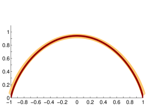
(a)

(b)

Figure 6.3: The Lyapunov profiles (dark red) on $[-1,1]$ and their approximations (light red circles) at time $560$ for two Exactly 1 examples, with doubly periodic initial states (a) $(10)^{\infty}$, and (b) $(1^{6}0^{2})^{\infty}$.

6.2.3 A Rule 110 example

Perhaps the most important example of our method is the Lyapunov profile for the Rule 110 ether [Coo]. This is a doubly periodic solution with $\sigma=14$, $\tau=7$, $\tau_{0}=1$, $\sigma_{0}=10$, and tile $1^{5}0^{3}10^{2}1^{2}0$. This ether supports a variety of gliders with complex interactions (in fact, as complex as possible [Coo]). As mentioned in Section 1, it remains unresolved whether, starting from the uniform product measure, the Lyapunov profile agrees with the one started from the ether. We now proceed to describe the latter profile. The expansion graph is rather sparse and is given in Table 6.2: for any $i$, and an edge $i\to j$, $j$ is given in the column corresponding to $D_{j}^{(i)}$ either $-1$, $0$ or $1$; these are the only displacement values and all corresponding $N_{j}^{(i)}=1$. Thus $d_{T}=26$.

Table 6.2: Specification for the graph $\mathcal{E}$ for the Rule 110 ether.

$i\in{\mathbb{Z}}_{\sigma}$	tile	$j$: $D_{j}^{(i)}=-1$	$j$: $D_{j}^{(i)}=0$	$j$: $D_{j}^{(i)}=1$
0	1	4		6
1	1		6	7
2	1	6	7	8
3	1	7	8
4	1	8	9
5	0	9	10
6	0	10	11
7	0	11
8	1	12	13
9	0		14
10	0	14		2
11	1	1
12	1		3
13	0	3	4	5

The profile, given in Fig. 6.4, is nonnegative on $[-8/9,2/3]$, vanishes at $2/3$ and equals $\log 3/9\approx 0.122$ at $-8/9$. The MLE equals about $0.647$ and is attained at the MLE direction about $-0.276$. We remark that the defect shape and values of $L$ at the boundaries, obtained here by a boundary analysis of defect dynamics, are closely connected to the spectral behavior of perturbed nilpotent matrices [EM].

Figure 6.4: The Lyapunov profile (dark red) on $[-1,1]$ and its approximation (light red circles) at time $560$ for the Rule 110 ether.

6.2.4 Variational principle in the reducible case

If $T^{\prime}$ is not essentially irreducible, but contains states that connect to several irreducible classes one can still characterize the Lyapunov profile by a variational principle, which is, however, multidimensional. We will state it below, but we first give two examples to show that the defect shape is not necessarily convex and that the defect profile is not necessarily a concave function. The simplest ECA example is Rule 184 with doubly periodic state with tile $01$ which has $\sigma=\pi=2$. This generates $W=\{-1,1\}$ with $L=0$ on $W$. For a simple example with $W=[-2,2]$, consider the CA with ${\mathcal{N}}=\{0,\pm 1,\pm 2\}$ and the update function given by $00101\mapsto 0$, $01011\mapsto 1$, and in all other cases $abcde\mapsto c$. Clearly, $(01)^{\infty}$ is a fixed point, thus has $\pi=1$. Also, it is easy to see that, provided that the support of $\Delta_{0}$ includes both an even integer and an odd integer, the profile is given by

$$L(\alpha)=\begin{cases}-\dfrac{|\alpha|}{2}\log\dfrac{|\alpha|}{2}-\left(1-\dfrac{|\alpha|}{2}\right)\log\left(1-\dfrac{|\alpha|}{2}\right)&\text{ if }|\alpha|\leq 2,\\ -\infty&\text{ otherwise. }\end{cases}$$

In this case the MLE equals $\log 2$, and in both examples there are two MLE directions, namely $\pm 1$.

Let $\mathcal{P}$ be the set of probability measures on $\{1,\ldots,d_{T}\}$. For a given $\alpha\in{\mathbb{R}}$, let

$$\mathcal{P}_{\alpha}=\{(\mu_{1},\ldots,\mu_{d_{T}})\in\mathcal{P}:\sum_{k}\mu_{k}D(e_{k})=\alpha\}.$$

Write $k\leadsto\ell$ if $k=\ell$ or $T^{n}_{k\ell}$ is positive for some $n$; that is, an oriented path in the graph $\mathcal{E}$ leads from edge $e_{k}$ to edge $e_{\ell}$. Moreover, for a given $b\in\{1,\ldots,d_{T}\}$, let

$$\mathcal{P}_{b}^{\prime}=\{(\mu_{1},\ldots,\mu_{d_{T}})\in\mathcal{P}: k,\ell\in\{1,\ldots,d_{T}\}$$ for all ,

$$\text{ if }b\not\leadsto k\text{ then }\mu_{k}=0\text{, and if }\ell\not\leadsto k\text{ and }k\not\leadsto\ell\text{ then }\mu_{k}\mu_{\ell}=0\}.$$

For any $\mu\in\mathcal{P}$, let $\mathcal{K}_{\mu}$ be the set of all $d_{T}\times d_{T}$ stochastic matrices $q=(q_{k\ell})$ that leave $\mu$ invariant, that is, they have positive entries and satisfy $\sum_{\ell}q_{k\ell}=1$, for all $k$, and $\sum_{k}\mu_{k}q_{k\ell}=\mu_{\ell}$, for all $\ell$. The expression that plays a role related to the relative entropy is the function $H$ defined on $\mathcal{K}\times\mathcal{P}$ by

$$H(q,\mu)=\sum_{k,\ell}\mu_{k}q_{k\ell}\log\frac{T_{k\ell}}{q_{k\ell}}.$$

Theorem 6.3.

Assume that a doubly periodic state $\eta$ is the initial CA state $\xi_{0}$. Fix also an initial set $\Delta_{0}$ and let

$$B_{0}=\{b\in\{1,\ldots,d_{T}\}:\text{ the edge }e_{b}\text{ originates from }x\operatorname{mod}\sigma\text{ for some }x\in\Delta_{0}\}.$$

Then the Lyapunov profile is proper and given by the following triple supremum

$$L(\alpha)=\sup_{b\in B_{0}}\,\,\,\sup_{\mu\in\mathcal{P}_{\alpha}\cap\mathcal{P}^{\prime}_{b}}\,\,\,\sup_{q\in\mathcal{K}_{\mu}}H(q,\mu).$$

Proof.

Assuming the defect paths must start with a fixed $b\in B_{0}$, the result follows from the general large deviation theorem for finite Markov chains (see Corollary 13.6 and Section 13.3 in [RS]) and the Contraction principle (Section 4.2.1 in [DZ]). Further, it is clear that the profile is obtained by the supremum over all possible choices of edges out of $\Delta_{0}$. ∎

7 Conclusions and open problems

The introduced non-equilibrium defect dynamics allows a simultaneous study of both the spatial extent and local accumulation of perturbations on a CA trajectory. The resulting Lyapunov profiles reveal quite a bit more information than the equilibrium version of Bagnoli et al. [BRR]. In particular, we provide a division of CA trajectories into three classes: in expansive cases defects spread (on the lattice and in their state space), in collapsing cases they die out, and in marginal cases they do neither of the two. Employing a mixture of rigorous and empirical methods, we classify all elementary CA starting from translation invariant product measures. We also make theoretical progress in the case of periodic initial conditions, where asymptotic shapes and large deviation rates are the main components of a Floquet theory for CA.

Our approach retains some of the spirit of the Wofram’s damage spreading [Wol1], although, as we have seen, it is fundamentally different and further insights into connections between the two would be welcome. In fact, the entire paper can be read as an invitation into a new topic with a wealth of intriguing open problems (many of which were mentioned in previous sections), and we conclude with a selection of them:

1. Can one prove that a CA trajectory has a proper Lyapunov profile under general conditions? Is there a simple example with a non-proper profile?

2. Can one understand which properties of a CA cause a phase transition between marginal and expansive dynamics as the initial density $p$ of $1$s varies, such as in the example at the end of Section 3? Can one determine the critical $p$ in that example?

3. For Rule 38 and other expansive stripes rules, is it possible to provide rigorous (numerical) bounds on the MLE and its direction?

4. For general stripes CA, can one prove, under proper conditions, the difference between $W$ and $W_{\text{\tt damage}}$ discussed in Section 3?

5. Is it possible to extend Theorem 4.1 to higher dimensions and thus give a general sufficient condition that a rule is marginal?

6. Does there exist a general algorithm to exactly determine the MLE for marginal CA, such as those in Table LABEL:ECA-marginal?

7. Can one prove that all rules in Table 4.4 are indeed expansive?

8. Is it possible to classify glider collisions for CA in Table 4.5 and then show that each rule belongs to the conjectured class?

9. Can a rigorous damage spreading theory be developed for periodic states?

10. Does the following version of irreducibility hold for all rules in Table 4.4: if $\xi_{0}$ is the uniform product measure and $A\subset{\mathbb{Z}}$ is finite, then either $L_{A}\equiv-\infty$ or $L_{A}=L_{\infty}$?

References

- [BD] J. M. Baetens, B. De Baets, Phenomenological study of irregular cellular automata based on Lyapunov exponents and Jacobians, Chaos 20 (2010), 033112, 1–15.
- [BER] F. Bagnoli, S. El Yacoubi, R. Rechtman, Control of cellular automata, Physical Review E 86 (2012), 066201–7, DOI: 10.1103/PhysRevE.86.066201.
- [BF] V. Belitsky, P. A, Ferrari, Ballistic annihilation and deterministic surface growth, Journal of Statistical Physics 80 (1995), 517–543.
- [BG] J. M. Baetens, J. Gravner, Introducing Lyapunov profiles of cellular automata, in “Proceedings of the 20th International Workshop on Cellular Automata and Discrete Complex Systems (AUTOMATA 2014) Himeji, Japan, July 2014,” T. Isokawa, K. Imai, N. Matsuin, F. Peper, and H. Umeo, editors, pp. 133–140. arXiv:1509.06639
- [Big] J. D. Biggins, The growth and spread of the general branching random walk, Annals of Applied Probability 5 (1995), 1008–1024.
- [BRR] F. Bagnoli, R. Rechtman, S. Ruffo, Damage spreading and Lyapunov exponents in cellular automata, Physics Letters A 172 (1992), 34–38.
- [BNT] M. Bramson, P. Ney, J. Tao, The population composition of a multitype branching random walk, Annals of Applied Probability 2 (1992), 519–765.
- [CK] M. Courbage, B. Kamiński, Space-time directional Lyapunov exponents for cellular automata, Journal of Statistical Physics 124 (2006) 1499–1509.
- [Coo] M. Cook, Universality in elementary cellular automata, Complex Systems 15 (2004), 1–40.
- [DS] R. Durrett, J. Steif, Some rigorous results for the Greenberg-Hastings model, Journal of Theoretical Probability (1991), 669–690.
- [DZ] A. Dembo, O. Zeitouni, Large Deviations Techniques and Applications, Second Edition. Springer, 1998.
- [EM] A. Edelman, Y. Ma, Non-generic eigenvalue perturbations of Jordan blocks, Linear Algebra and Applications 273 (1998), 45–63.
- [FMM] M. Finelli, G. Manzini, L. Margara, Lyapunov exponents versus expansivity and sensitivity in cellular automata Journal of Complexity 14 (1998), 210–233.
- [FS] S. Friedland, H. Schneider, The growth of powers of a nonnegative matrix, SIAM Journal on Algebraic Discrete Methods 1 (1980), 185–200.
- [Gig] M.-H. Giga, Y. Giga, Evolving graphs by singular weighted curvature, Archive for Rational Mechanics and Analysis 141 (1998), 117–198.
- [Gra1] P. Grassberger, Chaos and diffusion in deterministic cellular automata, Physica D 10 (1984), 52–58.
- [Gra2] P. Grassberger, Long-range effects in an elementary cellular automaton, Journal of Statistical Physics 45 (1986), 27–39.
- [GG1] J. Gravner, D. Griffeath, First passage times for discrete threshold growth dynamics, Annals of Probability 24 (1996), 1752–1778.
- [GG2] J. Gravner, D. Griffeath, Cellular automaton growth on : theorems, examples, and problems, Advances in Applied Mathematics 21 (1998), 241–304.
- [GG3] J. Gravner, D. Griffeath, Random growth models with polygonal shapes, Annals of Probability 34 (2006), 181–218.
- [GG4] J. Gravner, D. Griffeath, The one-dimensional Exactly 1 cellular automaton: replication, periodicity, and chaos from finite seeds, Journal of Statistical Physics 142 (2011), 168–200.
- [GG5] J. Gravner, D. Griffeath, Robust periodic solutions and evolution from seeds in one-dimensional edge cellular automata, Theoretical Computer Science 466 (2012), 64–86.
- [GH] J. Gravner, A. Holroyd, Percolation and disorder-resistance in cellular automata, Annals of Probability 43 (2015), 1731–1776.
- [Jen] E. Jen, Exact solvability and quasiperiodicity of one-dimensional cellular automata, Nonlinearity 4 (1991), 251–276.
- [LN] W. Li, M. G. Nordahl, Transient behavior of cellular automaton rule 110, Physics Letters A 166 (1992), 335–339.
- [Mar] G. J. Martinez, A note on elementary cellular automata classification, Journal of Cellular Automata 8 (2013), 233–259 .
- [Moo] G. Moore, Floquet theory as a computational tool, SIAM Journal on Numerical Analysis 42 (2004), 2522–2568.
- [MSZ] G. J. Martinez, J. C. Seck-Tuoh-Mora, H. Zenil, Computation and universality: Class IV versus Class III cellular automata, Journal of Cellular Automata 7 (2012), 393–430 .
- [RS] F. Rassoul-Agha, T. Seppäläinen, “A Course on Large Deviations with an Introduction to Gibbs Measures.” American Mathematical Society, Graduate Studies in Mathematics Volume 162, 2015.
- [Sch] R. H. Schonmann, Finite size scaling behavior of a biased majority rule cellular automaton, Physica A 167 (1990), 619–627.
- [She] M. A. Shereshevsky, Lyapunov exponents for one-dimensional cellular automata, Journal of Nonlinear Science 2 (1992), 1–8.
- [Tis1] P. Tisseur, Cellular automata and Lyapunov exponents, Nonlinearity 13 (2000), 1547–1560.
- [Tis2] P. Tisseur, Always finite entropy and Lyapunov exponents of two-dimensional cellular automata. arXiv:math/0502440
- [TM] T. Toffoli, N. Margolus, “Cellular Automata Machines.” MIT Press, 1991.
- [Vic1] G. Vichniac, Cellular automata models of disorder and organization, in “Disordered Systems and Biological Organization,” E. Bienenstock, F. Fogelman Soulié, G. Weisbuch, eds., Springer (1986), pp. 3–20.
- [Vic2] G. Vichniac, Boolean derivatives on cellular automata, Physica D 45 (1990), 63–74.
- [Wol1] S. Wolfram, Universality and complexity in cellular automata, Physica D 10 (1984), 1–35.
-
[Wol2]
S. Wolfram, The Wolfram Atlas: Elementary Cellular Automata,
http://atlas.wolfram.com/01/01/ - [Wil] S. J. Willson, On convergence of configurations, Discrete Mathematics 23 (1978), 279–300.
- [Yil] A. Yilmaz, Quenched large deviations for random walk in a random environment, Communications on Pure and Applied Mathematics 62 (2009), 1033–1075.
- [ZV] H. Zenil, E. Villareal-Zapata, Computation and universality: Class IV versus Class III cellular automata, International Journal of Bifurcation and Chaos 23 (2013), 18 pages, DOI: 10.1142/S0218127413501599.