A forward-backward view of some primal-dual optimization methods in image recovery

Abstract

A wide array of image recovery problems can be abstracted into the problem of minimizing a sum of composite convex functions in a Hilbert space. To solve such problems, primal-dual proximal approaches have been developed which provide efficient solutions to large-scale optimization problems. The objective of this paper is to show that a number of existing algorithms can be derived from a general form of the forward-backward algorithm applied in a suitable product space. Our approach also allows us to develop useful extensions of existing algorithms by introducing a variable metric. An illustration to image restoration is provided.

Keywords. convex optimization, duality, parallel computing, proximal algorithm, variational methods, image recovery.

1 Introduction

Many image recovery problems can be formulated in Hilbert spaces $\mathcal{H}$ and $(\mathcal{G}_{i})_{1\leqslant i\leqslant m}$ as structured optimization problems of the form

$$\underset{x\in\mathcal{H}}{\mathrm{minimize}}\;\;\sum_{i=1}^{m}g_{i}(L_{i}x),$$ (1)

where, for every $i\in\{1,\ldots,m\}$, $g_{i}$ is a proper lower semicontinuous convex function from $\mathcal{G}_{i}$ to $\,\left]-\infty,+\infty\right]$ and $L_{i}$ is a bounded linear operator from $\mathcal{H}$ to $\mathcal{G}_{i}$. For example, the functions $(g_{i}\circ L_{i})_{1\leqslant i\leqslant m}$ may model data fidelity terms, smooth or nonsmooth measures of regularity, or hard constraints on the solution. In recent years, many algorithms have been developed to solve such a problem by taking advantage of recent advances in convex optimization, especially in the development of proximal tools (see [12, 29] and the references therein). In image processing, however, solving such a problem still poses a number of conceptual and numerical challenges. First of all, one often looks for methods which have the ability to split the problem by activating each of the functions through elementary processing steps which can be computed in parallel. This makes it possible to reduce the complexity of the original problem and to benefit from existing parallel computing architectures. Secondly, it is often useful to design algorithms which can exploit, in a flexible manner, the structure of the problem. In particular, some of the functions may be Lipschitz differentiable in which case they should be exploited through their gradient rather than through their proximity operator, which is usually harder to implement (examples of proximity operators with closed-form expression can be found in [6, 12]). In some problems, the functions $(g_{i})_{1\leqslant i\leqslant m}$ can be expressed as the infimal convolution of simpler functions (see [9] and the references therein). Last but not least, in image recovery, the operators $(L_{i})_{1\leqslant i\leqslant m}$ may be of very large size so that their inversions are costly (e.g., in reconstruction problems). Finding algorithms which do not require to perform inversions of these operators is thus of paramount importance.

Note that all the existing convex optimization algorithms do not have these desirable properties. For example, the Alternating Direction Method of Multipliers (ADMM) [18, 17, 20] requires a stringent assumption of invertibility of the involved linear operator. Parallel versions of ADMM [28] and related Parallel Proximal Algorithm (PPXA) [11, 25] usually necessitate a linear inversion to be performed at each iteration. Also, early primal-dual algorithms [4, 5, 7, 10, 16, 21] did not make it possible to handle smooth functions through their gradients. Only recently, have primal-dual methods been proposed with this feature. Such work was initiated in [13] in the line of [4] and subsequent developments can be found in [2, 3, 8, 9, 15, 27, 30]. As will be seen in the present paper, another advantage of these approaches is that they can be coupled with variable metric strategies which can potentially accelerate their convergence.

In Section 2, we provide some background on convex analysis and monotone operator theory. In Section 3, we introduce a general form of the forward-backward algorithm which uses a variable metric. This algorithm is employed in Section 4 to develop a versatile family of primal-dual proximal methods. Several particular instances of this framework are discussed. Finally, we provide illustrating numerical results in Section 5.

2 Notation and background

Monotone operator theory [1] provides a both insightful and elegant framework for dealing with convex optimization problems and developing new solution algorithms that could not be devised using purely variational tools. We summarize a number of related concepts that will be needed.

Throughout, $\mathcal{H}$, $\mathcal{G}$, and $(\mathcal{G}_{i})_{1\leqslant i\leqslant m}$ are real Hilbert spaces. We denote the scalar product of a Hilbert space by $\left\langle{\cdot}\mid{\cdot}\right\rangle$ and the associated norm by $\|\cdot\|$. The symbol $\rightharpoonup$ denotes weak convergence, and $\operatorname{Id}$ denotes the identity operator. We denote by $\mathcal{B}\,(\mathcal{H},\mathcal{G})$ the space of bounded linear operators from $\mathcal{H}$ to $\mathcal{G}$, we set $\mathcal{S}\,(\mathcal{H})=\big{\{}{L\in\mathcal{B}\,(\mathcal{H},\mathcal{H})}\mid{L=L^{*}}\big{\}}$, where $L^{*}$ denotes the adjoint of $L$. The Loewner partial ordering on $\mathcal{S}\,(\mathcal{H})$ is denoted by $\succcurlyeq$. For every $\alpha\in\left[0,+\infty\right[$, we set $\mathcal{P}_{\alpha}(\mathcal{H})=\big{\{}{U\in\mathcal{S}\,(\mathcal{H})}\mid{U\succcurlyeq\alpha\operatorname{Id}}\big{\}},$ and we denote by $\sqrt{U}$ the square root of $U\in\mathcal{P}_{\alpha}(\mathcal{H})$. Moreover, for every $U\in\mathcal{P}_{\alpha}(\mathcal{H})$ and $\alpha>0$, we define the norm $\|x\|_{U}=\sqrt{\left\langle{Ux}\mid{x}\right\rangle}$.

We denote by $\boldsymbol{\mathcal{G}}=\mathcal{G}_{1}\oplus\cdots\oplus\mathcal{G}_{m}$ the Hilbert direct sum of the Hilbert spaces $(\mathcal{G}_{i})_{1\leqslant i\leqslant m}$, i.e., their product space equipped with the scalar product $\colon(\boldsymbol{x},\boldsymbol{y})\mapsto\sum_{i=1}^{m}\left\langle{x_{i}}\mid{y_{i}}\right\rangle$ where ${\boldsymbol{x}}=(x_{i})_{1\leqslant i\leqslant m}$ and ${\boldsymbol{y}}=(y_{i})_{1\leqslant i\leqslant m}$ denote generic elements in $\boldsymbol{\mathcal{G}}$.

Let $A\colon\mathcal{H}\to 2^{\mathcal{H}}$ be a set-valued operator. We denote by $\operatorname{gra}A=\big{\{}{(x,u)\in\mathcal{H}\times\mathcal{H}}\mid{u\in Ax}\big{\}}$ the graph of $A$, by $\operatorname{zer}A=\big{\{}{x\in\mathcal{H}}\mid{0\in Ax}\big{\}}$ the set of zeros of $A$, and by $\operatorname{ran}A=\big{\{}{u\in\mathcal{H}}\mid{(\exists\;x\in\mathcal{H})\;u\in Ax}\big{\}}$ its range. The inverse of $A$ is $A^{-1}\colon\mathcal{H}\mapsto 2^{\mathcal{H}}\colon u\mapsto\big{\{}{x\in\mathcal{H}}\mid{u\in Ax}\big{\}}$, and the resolvent of $A$ is $J_{A}=(\operatorname{Id}+A)^{-1}$. Moreover, $A$ is monotone if

$$(\forall(x,y)\in\mathcal{H}\times\mathcal{H})(\forall(u,v)\in Ax\times Ay)\;\;\left\langle{x-y}\mid{u-v}\right\rangle\geqslant 0,$$ (2)

and maximally monotone if it is monotone and there exists no monotone operator $B\colon\mathcal{H}\to 2^{\mathcal{H}}$ such that $\operatorname{gra}A\subset\operatorname{gra}B$ and $A\neq B$. An operator $B\colon\mathcal{H}\to\mathcal{H}$ is $\beta$-cocoercive for some $\beta\in\,\left]0,+\infty\right[$ if

$$(\forall x\in\mathcal{H})(\forall y\in\mathcal{H})\quad\left\langle{x-y}\mid{Bx-By}\right\rangle\geqslant\beta\|Bx-By\|^{2}.$$ (3)

The conjugate of a function $f\colon\mathcal{H}\to\,\left]-\infty,+\infty\right]$ is

$$f^{*}\colon\mathcal{H}\to\left[-\infty,+\infty\right]\colon u\mapsto\sup_{x\in\mathcal{H}}\big{(}\left\langle{x}\mid{u}\right\rangle-f(x)\big{)},$$ (4)

and the infimal convolution of $f$ with $g\colon\mathcal{H}\to\,\left]-\infty,+\infty\right]$ is

$$f\mbox{\footnotesize$\,\square\,$}g\colon\mathcal{H}\to\left[-\infty,+\infty\right]\colon x\mapsto\inf_{y\in\mathcal{H}}\big{(}f(y)+g(x-y)\big{)}.$$ (5)

The class of lower semicontinuous convex functions $f\colon\mathcal{H}\to\,\left]-\infty,+\infty\right]$ such that $\operatorname{dom}f=\big{\{}{x\in\mathcal{H}}\mid{f(x)<+\infty}\big{\}}\neq{\varnothing}$ is denoted by $\Gamma_{0}(\mathcal{H})$. If $f\in\Gamma_{0}(\mathcal{H})$, then $f^{*}\in\Gamma_{0}(\mathcal{H})$ and the subdifferential of $f$ is the maximally monotone operator

$$\partial f\colon \mathcal{H}\to 2^{\mathcal{H}}$$

$$x\mapsto\big{\{}{u\in\mathcal{H}}\mid{(\forall y\in\mathcal{H})\;\left\langle{y-x}\mid{u}\right\rangle+f(x)\leqslant f(y)}\big{\}}.$$ (6)

Let $U\in\mathcal{P}_{\alpha}(\mathcal{H})$ for some $\alpha\in\,\left]0,+\infty\right[$. The proximity operator of $f\in\Gamma_{0}(\mathcal{H})$ relative to the metric induced by $U$ is [22, Section XV.4]

$$\operatorname{prox}^{U}_{f}\colon\mathcal{H}\to\mathcal{H}\colon x\mapsto\underset{y\in\mathcal{H}}{\operatorname{argmin}}\>f(y)+\frac{1}{2}\|x-y\|_{U}^{2}.$$ (7)

When $U=\operatorname{Id}$, we retrieve the standard definition of the proximity operator [1, 24]. Let $C$ be a nonempty subset of $\mathcal{H}$. The indicator function of $C$ is defined on $\mathcal{H}$ as

$$\iota_{C}\colon x\mapsto\begin{cases}0,&\text{if}\;\;x\in C;\\ +\infty,&\text{if}\;\;x\notin C.\end{cases}$$ (8)

Finally, $\ell_{+}^{1}(\mathbb{N})$ denotes the set of summable sequences in $\left[0,+\infty\right[$.

3 A general form of Forward-Backward algorithm

Optimization problems can often be reduced to finding a zero of a sum of two maximally monotone operators $A$ and $B$ acting on $\mathcal{H}$. When $B$ is cocoercive (see (3)), a useful algorithm to solve this problem is the forward-backward algorithm, which can be formulated in a general form involving a variable metric as shown in the next result.

Theorem 3.1

Let $\alpha\in\,\left]0,+\infty\right[$, let $\beta\in\,\left]0,+\infty\right[$, let $A\colon\mathcal{H}\to 2^{\mathcal{H}}$ be maximally monotone, and let $B\colon\mathcal{H}\to\mathcal{H}$ be cocoercive. Let $(\eta_{n})_{n\in\mathbb{N}}\in\ell_{+}^{1}(\mathbb{N})$, and let $(V_{n})_{n\in\mathbb{N}}$ be a sequence in $\mathcal{P}_{\alpha}(\mathcal{H})$ such that

$$\begin{cases}\sup_{n\in\mathbb{N}}\|V_{n}\|<+\infty\\ (\forall n\in\mathbb{N})\quad(1+\eta_{n})V_{n+1}\succcurlyeq V_{n}\end{cases}$$ (9)

and $V_{n}^{1/2}BV_{n}^{1/2}$ is $\beta$-cocoercive. Let $(\lambda_{n})_{n\in\mathbb{N}}$ be a sequence in $\left]0,1\right]$ such that $\inf_{n\in\mathbb{N}}\lambda_{n}>0$ and let $(\gamma_{n})_{n\in\mathbb{N}}$ be a sequence in $]0,2\beta[$ such that $\inf_{n\in\mathbb{N}}\gamma_{n}>0$ and $\sup_{n\in\mathbb{N}}\gamma_{n}<2\beta$. Let $x_{0}\in\mathcal{H}$, and let $(a_{n})_{n\in\mathbb{N}}$ and $(b_{n})_{n\in\mathbb{N}}$ be absolutely summable sequences in $\mathcal{H}$. Suppose that $Z=\operatorname{zer}(A+B)\neq{\varnothing}$, and set

$$(\forall n\in\mathbb{N})\quad\begin{array}[]{l}\left\lfloor\begin{array}[]{l}y_{n}=x_{n}-\gamma_{n}V_{n}(Bx_{n}+b_{n})\\[2.84526pt] x_{n+1}=x_{n}+\lambda_{n}\big{(}J_{\gamma_{n}V_{n}A}\,(y_{n})+a_{n}-x_{n}\big{)}.\end{array}\right.\\[5.69054pt] \end{array}$$ (10)

Then $x_{n}\rightharpoonup\overline{x}$ for some $\overline{x}\in Z$.

At iteration $n$, variables $a_{n}$ and $b_{n}$ model numerical errors possibly arising when applying $J_{\gamma_{n}V_{n}A}$ or $B$. Note also that, if $B$ is $\mu$-cocoercive with $\mu\in\,\left]0,+\infty\right[$, one can choose $\beta=\mu(\sup_{n\in\mathbb{N}}\|V_{n}\|)^{-1}$, which allows us to retrieve [14, Theorem 4.1]. In the next section, we shall see how a judicious use of this result allows us to derive a variety of flexible convex optimization algorithms.

4 A variable metric primal-dual method

4.1 Formulation

A wide array of optimization problems encountered in image processing are instances of the following one, which was first investigated in [13] and can be viewed as a more structured version of the minimization problem in (1):

Problem 4.1

Let $z\in\mathcal{H}$, let $m$ be a strictly positive integer, let $f\in\Gamma_{0}(\mathcal{H})$, and let $h\colon\mathcal{H}\to\mathbb{R}$ be convex and differentiable with a Lipschitzian gradient. For every $i\in\{1,\ldots,m\}$, let $r_{i}\in\mathcal{G}_{i}$, let $g_{i}\in\Gamma_{0}(\mathcal{G}_{i})$, let $\ell_{i}\in\Gamma_{0}(\mathcal{G}_{i})$ be strongly convex, and suppose that $0\neq L_{i}\in\mathcal{B}\,(\mathcal{H},\mathcal{G}_{i})$. Suppose that

$$z\in\operatorname{ran}\bigg{(}\partial f+\sum_{i=1}^{m}L_{i}^{*}(\partial g_{i}\mbox{\footnotesize$\,\square\,$}\partial\ell_{i})(L_{i}\cdot-r_{i})+\nabla h\bigg{)}.$$ (11)

Consider the problem

$$\underset{\begin{subarray}{c}{x\in\mathcal{H}}\end{subarray}}{\mathrm{minimize}}\;\;f(x)+\sum_{i=1}^{m}\,(g_{i}\mbox{\footnotesize$\,\square\,$}\ell_{i})(L_{i}x-r_{i})+h(x)-\left\langle{x}\mid{z}\right\rangle,$$ (12)

and the dual problem

$$\underset{\begin{subarray}{c}{v_{1}\in\mathcal{G}_{1},\ldots,v_{m}\in\mathcal{G}_{m}}\end{subarray}}{\mathrm{minimize}}\;\; \big{(}f^{*}\mbox{\footnotesize$\,\square\,$}h^{*}\big{)}\bigg{(}z-\sum_{i=1}^{m}L_{i}^{*}v_{i}\bigg{)}$$

$$+\sum_{i=1}^{m}\big{(}g_{i}^{*}(v_{i})+\ell_{i}^{*}(v_{i})+\left\langle{v_{i}}\mid{r_{i}}\right\rangle\big{)}.$$ (13)

Note that in the special case when $\ell_{i}=\iota_{\{0\}}$, $g_{i}\mbox{\footnotesize$\,\square\,$}\ell_{i}$ reduces to $g_{i}$ in (12).

Let us now examine how Problem 4.1 can be reformulated from the standpoint of monotone operators. To this end, let us define $\boldsymbol{g}\in\Gamma_{0}(\boldsymbol{\mathcal{G}})$, $\boldsymbol{\ell}\in\Gamma_{0}(\boldsymbol{\mathcal{G}})$ and $\boldsymbol{L}\in\mathcal{B}\,(\mathcal{H},\boldsymbol{\mathcal{G}})$ by

$$\boldsymbol{g}\colon\boldsymbol{v}\mapsto\sum_{i=1}^{m}g_{i}(v_{i}),\qquad\boldsymbol{\ell}\colon\boldsymbol{v}\mapsto\sum_{i=1}^{m}\ell_{i}(v_{i})$$

and $$\boldsymbol{L}\colon x\mapsto(L_{1}x,\ldots,L_{m}x).$$ (14)

Let us now introduce the product space $\boldsymbol{\mathcal{K}}=\mathcal{H}\oplus\boldsymbol{\mathcal{G}}$ and the operators

$${\boldsymbol{A}}\colon\quad\;\;\boldsymbol{\mathcal{K}} \to 2^{\boldsymbol{\mathcal{K}}}$$

$$(x,\boldsymbol{v}) \mapsto(\partial f(x)-z+\boldsymbol{L}^{*}\boldsymbol{v})\times(-\boldsymbol{L}x+\partial\boldsymbol{g}^{*}(\boldsymbol{v})+\boldsymbol{r})$$ (15)

and

$${\boldsymbol{B}}\colon\quad\;\;\boldsymbol{\mathcal{K}} \to\boldsymbol{\mathcal{K}}$$

$$(x,\boldsymbol{v}) \mapsto\big{(}\nabla h(x),\nabla\boldsymbol{\ell}^{*}(\boldsymbol{v})\big{)}.$$ (16)

The operator ${\boldsymbol{A}}$ can be shown to be maximally monotone,whereas ${\boldsymbol{B}}$ is cocoercive. A key observation in this context is that, if there exists $(\overline{x},\overline{\boldsymbol{v}})\in\boldsymbol{\mathcal{K}}$ such that $(\overline{x},\overline{\boldsymbol{v}})\in\operatorname{zer}({\boldsymbol{A}}+{\boldsymbol{B}})$, then $(\overline{x},\overline{\boldsymbol{v}})$ is a pair of primal-dual solutions to Problem 4.1 [13]. This connection with the construction for a zero of ${\boldsymbol{A}}+{\boldsymbol{B}}$ makes it possible to apply a forward-backward algorithm as discussed in Section 3, by using a linear operator $\boldsymbol{V}_{n}\in\mathcal{B}\,(\boldsymbol{\mathcal{K}},\boldsymbol{\mathcal{K}})$ to change the metric at each iteration $n$. Depending on the form of this operator various algorithms can be obtained.

4.2 A first class of primal-dual algorithms

Let $\alpha\in\,\left]0,+\infty\right[$, let $(U_{n})_{n\in\mathbb{N}}$ be a sequence in $\mathcal{P}_{\alpha}(\mathcal{H})$ such that $(\forall n\in\mathbb{N})$ $U_{n+1}\succcurlyeq U_{n}$. For every $i\in\{1,\ldots,m\}$, let $(U_{i,n})_{n\in\mathbb{N}}$ be a sequence in $\mathcal{P}_{\alpha}(\mathcal{G}_{i})$ such that $(\forall n\in\mathbb{N})$ $U_{i,n+1}\succcurlyeq U_{i,n}$. A first possible choice for $(\boldsymbol{V}_{n})_{n\in\mathbb{N}}$ is given by

$$(\forall n\in\mathbb{N})\quad\boldsymbol{V}_{n}^{-1}\colon(x,\boldsymbol{v}) \mapsto(U_{n}^{-1}x-\boldsymbol{L}^{*}\boldsymbol{v},-\boldsymbol{L}x+\widetilde{\boldsymbol{U}}_{n}^{-1}\boldsymbol{v})$$ (17)

where

$$\widetilde{\boldsymbol{U}}_{n}\colon\boldsymbol{\mathcal{G}}\to\boldsymbol{\mathcal{G}}\colon(v_{1},\ldots,v_{m})\mapsto(U_{1,n}v_{1},\ldots,U_{m,n}v_{m}).$$ (18)

The following result constitutes a direct extension of [14, Example 6.4]:

Proposition 4.2

Let $x_{0}\in\mathcal{H}$, and let $(a_{n})_{n\in\mathbb{N}}$ and $(c_{n})_{n\in\mathbb{N}}$ be absolutely summable sequences in $\mathcal{H}$. For every $i\in\{1,\ldots,m\}$, let $v_{i,0}\in\mathcal{G}_{i}$, let $(b_{i,n})_{n\in\mathbb{N}}$ and $(d_{i,n})_{n\in\mathbb{N}}$ be absolutely summable sequences in $\mathcal{G}_{i}$. For every $n\in\mathbb{N}$, let $\mu_{n}\in\,\left]0,+\infty\right[$ be a Lipschitz constant of $U_{n}^{1/2}\circ\nabla h\circ U_{n}^{1/2}$ and, for every $i\in\{1,\ldots,m\}$, let $\nu_{i,n}\in\,\left]0,+\infty\right[$ be a Lipschitz constant of $U_{i,n}^{1/2}\circ\nabla\ell_{i}^{*}\circ U_{i,n}^{1/2}$. Let $(\lambda_{n})_{n\in\mathbb{N}}$ be a sequence in $]0,1]$ such that $\inf_{n\in\mathbb{N}}\lambda_{n}>0$. For every $n\in\mathbb{N}$, set

$$\delta_{n}=\Bigg{(}\sum_{i=1}^{m}\|\sqrt{U_{i,n}}L_{i}\sqrt{U_{n}}\|^{2}\Bigg{)}^{-1/2}-1,$$ (19)

and suppose that

$$\inf_{n\in\mathbb{N}}\frac{\delta_{n}}{(1+\delta_{n})\max\{\mu_{n},\nu_{1,n},\ldots,\nu_{m,n}\}}>\frac{1}{2}.$$ (20)

Set

$$\operatorname{For}\;n=0,1,\ldots$$

$$\begin{array}[]{l}\left\lfloor\begin{array}[]{l}p_{n}=\operatorname{prox}^{U^{-1}_{n}}_{f}\Big{(}x_{n}-U_{n}\big{(}\sum_{i=1}^{m}L_{i}^{*}v_{i,n}+\nabla h(x_{n})\\ \qquad\qquad\qquad\;\;+c_{n}-z\big{)}\Big{)}+a_{n}\\ y_{n}=2p_{n}-x_{n}\\ x_{n+1}=x_{n}+\lambda_{n}(p_{n}-x_{n})\\ \operatorname{For}\;i=1,\ldots,m\\ \left\lfloor\begin{array}[]{l}q_{i,n}=\operatorname{prox}^{U_{i,n}^{-1}}_{g_{i}^{*}}\Big{(}v_{i,n}+U_{i,n}\big{(}L_{i}y_{n}-\nabla\ell_{i}^{*}(v_{i,n})\\ \qquad\qquad\qquad\;\;\;\;-d_{i,n}-r_{i}\big{)}\Big{)}+b_{i,n}\\ v_{i,n+1}=v_{i,n}+\lambda_{n}(q_{i,n}-v_{i,n}).\\ \end{array}\right.\\[5.69054pt] \end{array}\right.\\[5.69054pt] \end{array}$$ (31)

Then $(x_{n})_{n\in\mathbb{N}}$ converges weakly to a solution to (12), for every $i\in\{1,\ldots,m\}$ $(v_{i,n})_{n\in\mathbb{N}}$ converges weakly to some $\overline{v}_{i}\in\mathcal{G}_{i}$, and $(\overline{v}_{1},\ldots,\overline{v}_{m})$ is a solution to (4.1).

In the special case when $U_{n}\equiv\tau\operatorname{Id}$ with $\tau\in\,\left]0,+\infty\right[$ and, for every $i\in\{1,\ldots,m\}$, $U_{i,n}\equiv\sigma_{i}\operatorname{Id}$ with $\sigma_{i}\in\,\left]0,+\infty\right[$, we recover the parallel algorithm proposed in [30]. Variants of this algorithm where, for every $i\in\{1,\ldots,m\}$, $\ell_{i}=\iota_{\{0\}}$ are also investigated in [15]. In this case, less restrictive assumptions on the choice of $(\tau,\sigma_{1},\ldots,\sigma_{m})$ can be made. Note that this algorithm itself can be viewed as a generalization of the algorithm which constitutes the main topic of [5, 16, 21] (designated by some authors as PDHG). A preconditioned version of this algorithm was proposed in [26] corresponding to the case when $m=1$, $(\forall n\in\mathbb{N})$ $U_{n}$ and $U_{1,n}$ are constant matrices, and no error term is taken into account. Algorithm (4.2) when, for every $n\in\mathbb{N}$, $\lambda_{n}\equiv 1$, $U_{n}$ and $(U_{i,n})_{1\leqslant i\leqslant m}$ are diagonal matrices, $h=0$, and $(\forall i\in\{1,\ldots,m\})$ $\ell_{i}=\iota_{\{0\}}$ appears also to be closely related to the adaptive method in [19].

4.3 A second class of primal-dual algorithms

Let $\alpha\in\,\left]0,+\infty\right[$, let $(U_{n})_{n\in\mathbb{N}}$ be a sequence in $\mathcal{P}_{\alpha}(\mathcal{H})$ such that $(\forall n\in\mathbb{N})$ $U_{n+1}\succcurlyeq U_{n}$. For every $i\in\{1,\ldots,m\}$, let $(U_{i,n})_{n\in\mathbb{N}}$ be a sequence in $\mathcal{P}_{\alpha}(\mathcal{G}_{i})$ such that $(\forall n\in\mathbb{N})$ $U_{i,n+1}\succcurlyeq U_{i,n}$. A second possible choice for $(\boldsymbol{V}_{n})_{n\in\mathbb{N}}$ is given by the following diagonal form:

$$(\forall n\in\mathbb{N})\quad\boldsymbol{V}_{n}^{-1}\colon(x,\boldsymbol{v}) \mapsto\big{(}U_{n}^{-1}x,(\widetilde{\boldsymbol{U}}_{n}^{-1}-\boldsymbol{L}U_{n}\boldsymbol{L}^{*})\boldsymbol{v}\big{)}$$ (32)

where $\widetilde{\boldsymbol{U}}_{n}$ is given by (18).

The following result can then be deduced from Theorem 3.1. Its proof is skipped due to the lack of space.

Proposition 4.3

Let $x_{0}\in\mathcal{H}$, and let $(c_{n})_{n\in\mathbb{N}}$ be an absolutely summable sequence in $\mathcal{H}$. For every $i\in\{1,\ldots,m\}$, let $v_{i,0}\in\mathcal{G}_{i}$, let $(b_{i,n})_{n\in\mathbb{N}}$ and $(d_{i,n})_{n\in\mathbb{N}}$ be absolutely summable sequences in $\mathcal{G}_{i}$. For every $n\in\mathbb{N}$, let $\mu_{n}\in\,\left]0,+\infty\right[$ be a Lipschitz constant of $U_{n}^{1/2}\circ\nabla h\circ U_{n}^{1/2}$ and, for every $i\in\{1,\ldots,m\}$, let $\nu_{i,n}\in\,\left]0,+\infty\right[$ be a Lipschitz constant of $U_{i,n}^{1/2}\circ\nabla\ell_{i}^{*}\circ U_{i,n}^{1/2}$. Let $(\lambda_{n})_{n\in\mathbb{N}}$ be a sequence in $]0,1]$ such that $\inf_{n\in\mathbb{N}}\lambda_{n}>0$. For every $n\in\mathbb{N}$, set

$$\zeta_{n}=1-\sum_{i=1}^{m}\|\sqrt{U_{i,n}}L_{i}\sqrt{U_{n}}\|^{2}$$ (33)

and suppose that

$$\inf_{n\in\mathbb{N}}\frac{\zeta_{n}}{\max\{\zeta_{n}\mu_{n},\nu_{1,n},\ldots,\nu_{m,n}\}}>\frac{1}{2}.$$ (34)

Set

$$\operatorname{For}\;n=0,1,\ldots$$

$$\begin{array}[]{l}\left\lfloor\begin{array}[]{l}s_{n}=x_{n}-U_{n}(\nabla h(x_{n})+c_{n}-z)\\ y_{n}=s_{n}-U_{n}\sum_{i=1}^{m}L_{i}^{*}v_{i,n}\\ \operatorname{For}\;i=1,\ldots,m\\ \left\lfloor\begin{array}[]{l}q_{i,n}=\operatorname{prox}^{U_{i,n}^{-1}}_{g_{i}^{*}}\Big{(}v_{i,n}+U_{i,n}\big{(}L_{i}y_{n}-\nabla\ell_{i}^{*}(v_{i,n})\\ \qquad\qquad\qquad\;\;\;\;-d_{i,n}-r_{i}\big{)}\Big{)}+b_{i,n}\\ v_{i,n+1}=v_{i,n}+\lambda_{n}(q_{i,n}-v_{i,n}).\\ \end{array}\right.\\[5.69054pt] p_{n}=s_{n}-U_{n}\sum_{i=1}^{m}L_{i}^{*}q_{i,n}\\ x_{n+1}=x_{n}+\lambda_{n}(p_{n}-x_{n}).\\ \end{array}\right.\\[5.69054pt] \end{array}$$ (45)

Assume that $f=0$. Then $(x_{n})_{n\in\mathbb{N}}$ converges weakly to a solution to (12), for every $i\in\{1,\ldots,m\}$ $(v_{i,n})_{n\in\mathbb{N}}$ converges weakly to some $\overline{v}_{i}\in\mathcal{G}_{i}$, and $(\overline{v}_{1},\ldots,\overline{v}_{m})$ is a solution to (4.1).

The algorithm proposed in [23, 8] is a special case of the previous one, in the absence of errors, when $m=1$, $\mathcal{H}$ and $\mathcal{G}_{1}$ are finite dimensional spaces, $\ell_{1}=\iota_{\{0\}}$, $U_{n}\equiv\tau\operatorname{Id}$ with $\tau\in\,\left]0,+\infty\right[$, $U_{1,n}\equiv\sigma\operatorname{Id}$ with $\sigma\in\,\left]0,+\infty\right[$, and no relaxation ($\lambda_{n}\equiv 1)$ or a constant one ($\lambda_{n}\equiv\kappa<1$) is performed.

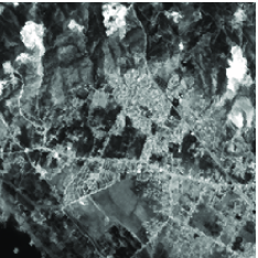
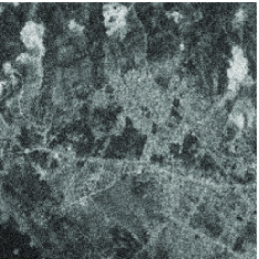
(a)	(b)
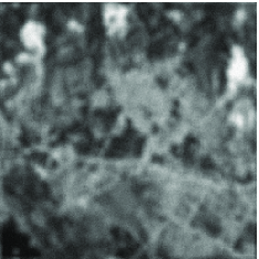
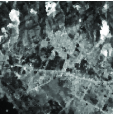
(c)	(d)

Figure 1: Original image $\overline{x}$ (a), noisy image $w_{1}$ (SNR = $5.87$ dB) (b), blurred image $w_{2}$ (SNR = $16.63$ dB) (c), and restored image $\widetilde{x}$ (SNR = $21.61$ dB) (d).

5 Application to image restoration

We illustrate the flexibility of the proposed primal-dual algorithms on an image recovery example. Two observed images $w_{1}$ and $w_{2}$ of the same scene $\overline{x}\in\mathbb{R}^{N}$ ($N=256^{2}$) are available (see Fig. 1(a)-(c)). The first one is corrupted with a noise with a variance $\theta_{1}^{2}=576$, while the second one has been degraded by a linear operator $H\in\mathbb{R}^{N\times N}$ ($7\times 7$ uniform blur) and a noise with variance $\theta_{2}^{2}=25$. The noise components are mutually statistically independent, additive, zero-mean, white, and Gaussian distributed. Note that this kind of multivariate restoration problem is encountered in some push-broom satellite imaging systems.

An estimate $\widetilde{x}$ of $\overline{x}$ is computed as a solution to (12) where $m=2$, $z=0$, $r_{1}=0$, $r_{2}=0$,

$$h =\frac{1}{\theta_{1}^{2}}\|\cdot-w_{1}\|^{2}+\frac{1}{\theta_{2}^{2}}\|H\cdot-w_{2}\|^{2},$$ (46)

$$g_{1} =\iota_{[0,255]^{N}},\quad g_{2}=\kappa\|\cdot\|_{1,2},$$ (47)

$$f =0,\quad\ell_{1}=\ell_{2}=\iota_{\{0\}}$$ (48)

where the second function in (47) denotes the $\ell_{1,2}$-norm and $\kappa\in\,\left]0,+\infty\right[$. In addition, $L_{1}=\operatorname{Id}$ and $L_{2}=[G_{1}^{\top},G_{2}^{\top}]^{\top}$ where $G_{1}\in\mathbb{R}^{N\times N}$ and $G_{2}^{N\times N}$ are horizontal and vertical discrete gradient operators. Function $g_{1}$ introduces some a priori constraint on the range values in the target image, while function $g_{2}\circ L_{2}$ corresponds to a classical total variation regularization. The minimization problem is solved numerically by using Algorithm (4.3) with $\lambda_{n}\equiv 1$. In a first experiment, standard choices of the algorithm parameters are made by setting $U_{n}\equiv\tau\operatorname{Id}$, $U_{1,n}\equiv\sigma_{1}\operatorname{Id}$, and $U_{2,n}=\sigma_{2}\operatorname{Id}$ with $(\tau,\sigma_{1},\sigma_{2})\in\,\left]0,+\infty\right[^{3}$. In a second experiment, a more sophisticated choice of the metric is made. The operators $(U_{n})_{n\in\mathbb{N}}$, $(U_{1,n})_{n\in\mathbb{N}}$ and $(U_{2,n})_{n\in\mathbb{N}}$ are still chosen diagonal and constant in order to facilitate the implementation of the algorithm, but the diagonal values are optimized in an empirical manner. A similar strategy was applied in [26] in the case of Algorithm (4.2). The regularization parameter $\kappa$ has been set so as to get the highest value of the resulting signal-to-noise ratio (SNR).

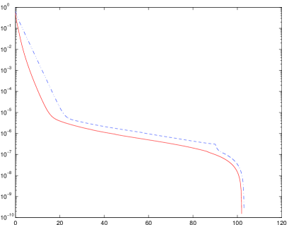
Figure 2: Normalized norm of the error on the iterate vs computation time (in seconds) for Experiment 1 (blue, dash dot line) and Experiment 2 (red, continuous line).

The restored image is displayed in Fig. 1(d). Fig. 2 shows the convergence profile of the algorithm. We plot the evolution of the normalized Euclidean distance (in log scale) between the iterates and $\widetilde{x}$ in terms of computational time (Matlab R2011b codes running on a single-core Intel i7-2620M CPU@2.7 GHz with 8 GB of RAM). An approximation of $\widetilde{x}$ obtained after 5000 iterations is used. This result illustrates the fact that an appropriate choice of the metric may be beneficial in terms of speed of convergence.

References

• [1] H. H. Bauschke and P. L. Combettes, Convex Analysis and Monotone Operator Theory in Hilbert Spaces.   New York: Springer, 2011.
• [2] S. R. Becker and P. L. Combettes, “An algorithm for splitting parallel sums of linearly composed monotone operators, with applications to signal recovery,” Nonlinear Convex Anal., vol. 15, no. 1, pp. 137–159, Jan. 2014.
• [3] R. I. Boţ and C. Hendrich, “Convergence analysis for a primal-dual monotone + skew splitting algorithm with applications to total variation minimization,” J. Math. Imaging Vision, 2013, accepted http://www.mat.univie.ac.at/$\sim$rabot/publications/jour13-18.pdf.
• [4] L. M. Briceño-Arias and P. L. Combettes, “A monotone + skew splitting model for composite monotone inclusions in duality,” SIAM J. Optim., vol. 21, no. 4, pp. 1230–1250, Oct. 2011.
• [5] A. Chambolle and T. Pock, “A first-order primal-dual algorithm for convex problems with applications to imaging,” J. Math. Imaging Vision, vol. 40, no. 1, pp. 120–145, 2011.
• [6] C. Chaux, P. L. Combettes, J.-C. Pesquet, and V. R. Wajs, “A variational formulation for frame-based inverse problems,” Inverse Problems, vol. 23, no. 4, pp. 1495–1518, Jun. 2007.
• [7] G. Chen and M. Teboulle, “A proximal-based decomposition method for convex minimization problems,” Math. Program., vol. 64, pp. 81–101, 1994.
• [8] P. Chen, J. Huang, and X. Zhang, “A primal-dual fixed point algorithm for convex separable minimization with applications to image restoration,” Inverse Problems, vol. 29, no. 2, 2013, doi:10.1088/0266-5611/29/2/025011.
• [9] P. L. Combettes, “Systems of structured monotone inclusions: duality, algorithms, and applications,” SIAM J. Optim., vol. 23, no. 4, pp. 2420–2447, Dec. 2013.
• [10] P. L. Combettes, D. Dũng, and B. C. Vũ, “Dualization of signal recovery problems,” Set-Valued Var. Anal., vol. 18, pp. 373–404, Dec. 2010.
• [11] P. L. Combettes and J.-C. Pesquet, “A proximal decomposition method for solving convex variational inverse problems,” Inverse Problems, vol. 24, no. 6, Dec. 2008.
• [12] ——, “Proximal splitting methods in signal processing,” in Fixed-Point Algorithms for Inverse Problems in Science and Engineering, H. H. Bauschke, R. S. Burachik, P. L. Combettes, V. Elser, D. R. Luke, and H. Wolkowicz, Eds.   New York: Springer-Verlag, 2011, pp. 185–212.
• [13] ——, “Primal-dual splitting algorithm for solving inclusions with mixtures of composite, Lipschitzian, and parallel-sum type monotone operators,” Set-Valued Var. Anal., vol. 20, no. 2, pp. 307–330, June 2012.
• [14] P. L. Combettes and B. C. Vũ, “Variable metric forward-backward splitting with applications to monotone inclusions in duality,” Optimization, 2012, published online DOI:10.1080/02331934.2012.733883.
• [15] L. Condat, “A primal-dual splitting method for convex optimization involving Lipschitzian, proximable and linear composite terms,” J. Optim. Theory Appl., vol. 158, no. 2, pp. 460–479, Aug. 2013.
• [16] E. Esser, X. Zhang, and T. Chan, “A general framework for a class of first order primal-dual algorithms for convex optimization in imaging science,” SIAM J. Imaging Sci., vol. 3, no. 4, pp. 1015–1046, 2010.
• [17] M. A. T. Figueiredo and R. D. Nowak, “Deconvolution of Poissonian images using variable splitting and augmented Lagrangian optimization,” in IEEE Work. on Stat. Sig. Proc., Cardiff, United Kingdom, Aug. 31 - Sept. 3 2009, pp. x-x+4.
• [18] M. Fortin and R. Glowinski, Eds., Augmented Lagrangian Methods: Applications to the Numerical Solution of Boundary-Value Problems.   Amsterdam: North-Holland: Elsevier Science Ltd, 1983.
• [19] T. Goldstein, E. Esser, and R. Baraniuk, “Adaptive primal-dual hybrid gradient methods for saddle-point problems,” 2013, http://arxiv.org/abs/1305.0546.
• [20] T. Goldstein and S. Osher, “The split Bregman method for $\ell_{1}$-regularized problems,” SIAM J. Imaging Sci., vol. 2, pp. 323–343, 2009.
• [21] B. He and X. Yuan, “Convergence analysis of primal-dual algorithms for a saddle-point problem: from contraction perspective,” SIAM J. Imaging Sci., vol. 5, no. 1, pp. 119–149, 2012.
• [22] J.-B. Hiriart-Urruty and C. Lemaréchal, Convex Analysis and Minimization Algorithms, Part II : Advanced Theory and Bundle Methods.   New York: Springer-Verlag, 1993.
• [23] I. Loris and C. Verhoeven, “On a generalization of the iterative soft-thresholding algorithm for the case of non-separable penalty,” Inverse Problems, vol. 27, no. 12, p. 125007, 2011.
• [24] J.-J. Moreau, “Proximité et dualité dans un espace hilbertien,” Bull. Soc. Math. France, vol. 93, pp. 273–299, 1965.
• [25] J.-C. Pesquet and N. Pustelnik, “A parallel inertial proximal optimization method,” Pac. J. Optim., vol. 8, no. 2, pp. 273–305, Apr. 2012.
• [26] T. Pock and A. Chambolle, “Diagonal preconditioning for first order primal-dual algorithms in convex optimization,” in Proc. IEEE Int. Conf. Comput. Vis., Barcelona, Spain, Nov. 6-13 2011, pp. 1762–1769.
• [27] A. Repetti, E. Chouzenoux, and J.-C. Pesquet, “A penalized weighted least squares approach for restoring data corrupted with signal-dependent noise,” in Proc. Eur. Sig. and Image Proc. Conference, Bucharest, Romania, 27-31 Aug. 2012, pp. 1553–1557.
• [28] S. Setzer, G. Steidl, and T. Teuber, “Deblurring Poissonian images by split Bregman techniques,” J. Visual Communication and Image Representation, vol. 21, no. 3, pp. 193–199, Apr. 2010.
• [29] S. Sra, S. Nowozin, and S. J. Wright, Optimization for Machine Learning.   Cambridge, MA: MIT Press, 2012.
• [30] B. C. Vũ, “A splitting algorithm for dual monotone inclusions involving cocoercive operators,” Adv. Comput. Math., vol. 38, no. 3, pp. 667–681, Apr. 2013.