Cosmological Applications of the Gaussian Kinematic Formula

Abstract

The Gaussian Kinematic Formula (GKF, see Adler and Taylor (2007,2011)) is an extremely powerful tool allowing for explicit analytic predictions of expected values of Minkowski functionals under realistic experimental conditions for cosmological data collections. In this paper, we implement Minkowski functionals on multipoles and needlet components of CMB fields, thus allowing a better control of cosmic variance and extraction of information on both harmonic and real domains; we then exploit the GKF to provide their expected values on spherical maps, in the presence of arbitrary sky masks, and under nonGaussian circumstances. All our results are validated by numerical experiments, which show a perfect agreement between theoretical predictions and Monte Carlo simulations.

I Introduction

A general trend in modern cosmological research is the implementation of more and more sophisticated statistical tools to perform data analysis. Indeed, as well-known cosmological data have reached over the last decade an unprecedented accuracy, so that it has become customary to speak about a golden era for Cosmology, featuring a data deluge from a bunch of satellite - and ground based-experiments. As the data grow in size and precision, more and more detailed questions can be addressed, and exploiting techniques at the frontier of statistical and mathematical research becomes mandatory to warrant a full exploration of the available evidence.

Among these techniques, stochastic geometry tools have now become very well established, especially in the field of Cosmic Microwave Background radiation experiments. In this area, one of the most popular geometric tools for data analysis are certainly the so-called Minkowski functionals (MFs), which have been extensively exploited as tools to search for nonGaussianities, anisotropies, asymmetries and other features of CMB data. The use of MFs in Cosmology goes back at least to Tomita (1986); Coles (1988); a complete bibliography would certainly include hundreds of entries, so we refer only to the earlier works by Schmalzing and Buchert (1997); Dolgov et al. (1999); Naselsky and Novikov (1998); Novikov et al. (2000); Schmalzing and Gorski (1998); Matsubara (2003); Komatsu et al. (2003); Spergel et al. (2007) and to the more recent ones by Natoli et al. (2010); Matsubara (2010); Ducout et al. (2013); Pratten and Munshi (2012); Munshi et al. (2013); Planck Collaboration et al. (2013).

As well-known, on the plane there are three Minkowski functionals M${}_{0},$M${}_{1},$M₂ which can be taken to represent, respectively, the area, the boundary length and the Euler-Poincaré characteristic (number of connected components minus holes) of any given region. To characterize the behaviour of data from a random field ($T(x),$ say) it is has then become customary to consider flat-sky approximations and to focus on the excursion sets

$$A_{u}(T):=\left\{x:T(x)>u\right\}\text{ ,}$$

e.g. the regions of the plane where the value of $T$ exceeds the threshold $u;$ the corresponding functionals M${}_{i}(A_{u}(T)),$ $i=0,1,2$, can then be computed for real data with a number of accurate and numerically efficient packages. The expected values of the Minkowski functionals in the planar case and under Gaussianity is analytically known to the literature since the work of Adler in the early 80’s (Adler (1981), see also Tomita (1986)), and these predictions can be compared to values on observed data to implement a number of statistical tests (see for instance Planck Collaboration et al. (2013) and the references therein).

In the last decade, some major progresses have occurred in the mathematical understanding of the geometry of random fields, namely the discovery of the Gaussian Kinematic Formula by Taylor and Adler (see Taylor and Adler (2003); Taylor (2006); Adler et al. (2009), Adler and Taylor (2011), Adler and Taylor (2007)).

As we shall discuss in the next section, the Gaussian kinematic formula allows a simple computation of the expected values for Lipschitz-Killing curvatures (equivalent to Minkowski functionals, see below) under an impressive variety of extremely different circumstances, covering arbitrary manifolds with and without masked regions and a broad class of nonGaussian models. These expected values take extremely neat and intuitive forms, and can be immediately compared to simulations and observed data. One of our purposes in this paper is to exploit these recent results to develop a number of analytic predictions on functionals tailored to test nonGaussianities and asymmetries on CMB data.

More precisely, in this paper we aim at the implementation of Minkowski functionals/Lipschitz-Killing curvatures on the multipole and needlet components of observed data. To be more explicit, we start from the decomposition of an observed spherical (e.g., CMB) map into harmonics as

$$T(x)=\sum_{\ell=1}^{L_{\max}}\sum_{m=-\ell}^{\ell}a_{\ell m}Y_{\ell m}(x)=\sum_{\ell=1}^{L_{\max}}T_{\ell}(x)\text{ ;}$$ (1)

It is well-known that the decomposition (1) is only feasible for unmasked (full-sky) data, a condition which is usually considered very difficult to meet for CMB experiments (see, however, the recent full-sky maps produced by Bobin et al. (2014)). To handle masked regions, it has hence become very popular to introduce various forms of spherical wavelets, which enjoy much better localization properties than spherical harmonics in the real domain, and are therefore much less affected by sky cuts. In this paper, we shall focus in particular on the needlet system, which is defined by the filter

$$\psi_{jk}(x)=\sum_{\ell,m}b(\frac{\ell}{B^{j}})\overline{Y}_{\ell m}(\xi_{jk})Y_{\ell m}(x)\text{ ,}$$

where $\left\{\xi_{jk}\right\}$ denotes a grid of points on the sphere (such as HealPix centers at a given resolution, see Górski et al. (2005)), $B>1$ is some fixed bandwidth parameter and the weight function $b(\frac{\ell}{2^{j}})$ satisfies three conditions, namely a) it is compactly supported in the interval ($B^{-1},B);$ b) it is smooth; c) the partition of unity property holds, e.g. $\sum_{j}b^{2}(\frac{\ell}{B^{j}})=1$ for all $\ell.$ Needlets have been shown to enjoy very good localization properties in the real domain; needlet coefficients are given by the projection

$$\beta_{jk}=\int_{S^{2}}T(x)\psi_{jk}(x)dx=\sum_{\ell=B^{j-1}}^{B^{j+1}}\sum_{m}b(\frac{\ell}{B^{j}})a_{\ell m}Y_{\ell m}(\xi_{jk})\text{ ,}$$

and they allow for the reconstruction formula

$$T(x) = \sum_{j=1}^{J_{\max}}\sum_{k}\beta_{jk}\psi_{jk}(x)=\sum_{j=1}^{J_{\max}}\beta_{j}(x)\text{ , }$$ (2)

$$\beta_{j}(x) = \sum_{k}\beta_{jk}\psi_{jk}(x)=\sum_{\ell=B^{j-1}}^{B^{j+1}}\sum_{m}b^{2}(\frac{\ell}{B^{j}})a_{\ell m}Y_{\ell m}(x)\text{ ,}$$

see Narcowich et al. (2006), Baldi et al. (2009a), Marinucci et al. (2008), Donzelli et al. (2012) for further discussions and applications to some CMB data analysis issues.

Our aim is to apply Minkowski functionals on both the field components $\left\{T_{\ell}(x),\beta_{j}(x)\right\}$ rather than on the original map. This form of harmonic/needlet space geometric analysis has a number of advantages that it is immediate to see (see also Marinucci and Vadlamani (2013) for some mathematical results in this area). For instance, any deviation from the analytic predictions can be exactly localized on the real and harmonic space, thus allowing for a much neater interpretation; indeed, a scale-by-scale probe of asymmetries and relevant features becomes feasible. Also, while the behaviour of MFs on standard CMB maps is unavoidably affected by Cosmic Variance, the effect is much smaller for MFs evaluated on the highest needlet scales: it becomes possible to discriminate quite clearly cosmic variance effects from effective deviations. Indeed, the variances of these Minkowski functionals converge to zero as the frequency increases, so that fluctuations around expected values become negligible on small scales, assuming the null assumptions hold. This allows for a very precise investigation of asymmetries and anisotropies; in a future work we shall provide some exact computations on the variances of these functionals and corresponding aggregated statistics.

The plan of the paper is as follows: in Section 2, we illustrate some background material on the Gaussian Kinematic Formula and we present its application to needlet and multipole components under the simplest conditions, e.g., full-sky Gaussian maps. In Section 3 we present analytic results for some nonGaussian fields arising when testing for asymmetries and directional variations in nonGaussianity, while Section 4 is devoted to the formulae for the exact expected values in the presence of masked regions. In Section 5 we present our detailed numerical studies, and we illustrate our software which allows for numerical corrections of expected values in the presence of masked regions of any form. Section 6 draws some conclusions and presents directions for future work.

II The Gaussian Kinematic Formula

II.1 The general case

For cosmological applications, it would seem sufficient to restrict our attention to random fields or observational data on the unit sphere $S^{2};$ however we shall show below that presenting results in a more general setting does yield some practical advantages, especially when dealing with masked data. Indeed, the Gaussian Kinematic Formula holds in much greater generality, and it can certainly be exploited for other experimental setups, for instance three-dimensional observations (viewed as data on the three-dimensional ball - this and other cases will be the object of future works).

On the sphere, the excursion sets $A_{u}(f)$ of a given (possibly random) function $f$ are defined as

$$A_{u}(f):=\left\{x\in S^{2}:f(x)\geq u\right\}\text{ .}$$

Of course, in the limit where we take $u=-\infty,$ we have that $A_{u}(f)=S^{2}$.

The Lipschitz-Killing Curvatures (LKCs) of these excursion sets, written

$$\mathcal{L}_{0}(A_{u}(f)),\mathcal{L}_{1}(A_{u}(f)),\mathcal{L}_{2}(A_{u}(f))$$

are defined as:

• $\mathcal{L}_{0}(A_{u}(f))$ is the Euler-Poincaré characteristic, e.g. in two dimensions the number of connected regions minus the number of holes, and in three dimensions the number of connected components, minus the number of ”handles” plus the number of holes, see Adler and Taylor (2011) for more discussion. This corresponds to the third Minkowski functional, or two minus the genus; we recall that the Euler-Poincaré characteristic of the full sphere is equal to two.

• $\mathcal{L}_{1}(A_{u}(f))$ is half the boundary length of the excursion regions, e.g. the second Minkowski functional up to a factor 2. For the full sphere, the boundary length is clearly zero

• $\mathcal{L}_{2}(A_{u}(f))$ is the area of the excursion regions, e.g. the first Minkowski functional. For the full sphere, one obviously gets $4\pi$.

For more general manifolds, the definitions are given in the Appendix. We shall focus on random fields that have zero mean, unit variance and are isotropic. These assumptions can be easily abandoned, entailing just a more complex notation; of course, zero mean and unit variance can be enforced by normalization (incidentally, it is well-known that needlet and multipole components random fields have always zero mean under isotropy). Let us now introduce some more notation; consider the family of functions $\rho_{l}(u)$ given by

$$\rho_{l}(u)=(2\pi)^{-(l+1)/2}H_{l-1}(u)e^{-u^{2}/2}\text{ ,}$$

where $H_{k}(u)$ denotes standard Hermite polynomials, e.g.,

$$H_{0}(u)=1,H_{1}(u)=u,H_{2}(u)=u^{2}-1;$$

we adopt the standard convention that

$$H_{-1}(u)=\sqrt{2\pi}(1-\Phi(u))e^{u^{2}/2},$$

where $\Phi(u)$ is the standard Gaussian c.d.f., so that

$$\rho_{0}(u) = (2\pi)^{-1/2}\sqrt{2\pi}(1-\Phi(u))e^{u^{2}/2}e^{-u^{2}/2}=(1-\Phi(u))$$

$$\rho_{1}(u) = \frac{1}{2\pi}e^{-u^{2}/2}\text{ , }\rho_{2}(u)=\frac{1}{\sqrt{(2\pi)^{3}}}ue^{-u^{2}/2}.$$

It is interesting to note that $\frac{1}{\sqrt{2\pi}}H_{k}(u)e^{-u^{2}/2}$ gives $(-1)^{k}$ times the $k$-th derivative of a standard Gaussian density, $k\geq 0.$ In the mathematical literature, this component is written as $\mathcal{M}_{l}^{\gamma}([u,\infty))=\frac{1}{\sqrt{2\pi}}H_{k}(u)e^{-u^{2}/2}$ and labelled a Gaussian Minkowski functional. This terminology, however, may result quite misleading in a CMB framework, because Gaussian Minkowski functionals are not at all the same as the Minkowski functionals for Gaussian fields: hereafter hence we will not use this jargon.

The next ingredient we shall need are the so-called ”flag” coefficients, which are given by

$$\left[\begin{array}[]{c}i+l\\ l\end{array}\right]=\left(\begin{array}[]{c}i+l\\ l\end{array}\right)\frac{\omega_{i+l}}{\omega_{i}\omega_{l}}\text{ , for }\omega_{i}=\frac{\pi^{i/2}}{\Gamma(\frac{i}{2}+1)}\text{ ,}$$

so that $\omega_{i}$ represents the area of the $i-$dimensional unit ball, $\omega_{1}=2,$ $\omega_{2}=\pi,$ $\omega_{3}=\frac{4}{3}\pi.$ Finally, we shall introduce a parameter $\lambda$, which represents the variance of any gradient component at the origin; equivalently $\lambda$ is simply given by the second derivative of the covariance function at the origin.

Under these circumstances, for random fields defined on general manifolds $D$ the Gaussian Kinematic Formula is given by the following, extremely elegant expression (see for instance Theorem 13.2.1 Adler and Taylor (2007):

$$\lambda^{i/2}\mathbb{E}\mathcal{L}_{i}(A_{u}(T(x),D))=\sum_{l=0}^{\dim(D)-i}\left[\begin{array}[]{c}i+l\\ l\end{array}\right]\lambda^{(i+l)/2}\rho_{l}(u)\mathcal{L}_{i+l}(D)\text{ .}$$ (3)

This expression may seem unnecessarily complicated, given that in this paper we shall focus only on spherical random fields: however this generality will indeed be required below, when we shall consider masked data (which we will see as data sampled from a different manifold, i.e. the sphere with sky-cuts). Before we proceed, however, it is important to stress some crucial features of the result given in (3). Indeed, it must be noted that the expression on the right-hand side of (3) allows for a full decoupling of the expected value on the left-hand side into components which are completely independent: the LKCs of the original manifold $\mathcal{L}_{k}(D),$ which depend on the manifold $D$ but not by the threshold value $u$ nor on the covariance structure of the field we investigate; and the functions $\rho_{l}(u),$ which depend only on the chosen threshold level $u$, and are independent from the structure of the field nor from the properties of the manifold $D$. This will allow for enormous computational advantages in the sections to follow: for instance, covering the presence of sky-cuts will entail a new computation for the values of $\mathcal{L}_{i+l}(D),$ which can be given once for all for a given mask; this computation will not be influenced, however, by threshold levels or correlation structure. Likewise, moving to nonGaussian circumstances will entail a corresponding replacement of the functions $\rho_{l}(u),$ but no new computations will be required on correlation structure or to handle gaps. A particular neat interpretation can be provided, by simply grouping together the terms $\lambda^{k/2}\$ and $\mathcal{L}_{k}(D),$ to obtain

$$\mathcal{L}_{k}^{T}(D)=\lambda^{k/2}\mathcal{L}_{k}(D)\text{ ;}$$

in mathematical terms, $\mathcal{L}_{k}^{T}(D)$ is usually described as a LKC computed with a metric induced by the random field $T,$ e.g. a manifold which has been rescaled by multiplication times $\sqrt{\lambda},$ the square root of the second derivative of its covariance function at the origin. All these notions may seem somewhat abstract, but they yield very simple analytic expressions in the case of spherical random fields $D=S^{2},$ to which we now turn our attention.

II.2 The spherical case

An example of excursion regions of the CMB for different threshold levels is given by Figure (1).

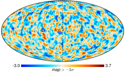
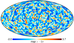
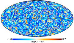
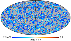
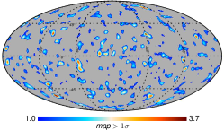
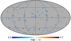
Figure 1: Illustration of excursion fields on a CMB map. The original map is smoothed by a $5^{\circ}$ beam. The subtitles below the color bar indicate the threshold levels.

The application of the previous general results to the sphere (without masks) basically provides expression which are already known to the CMB literature, up to some correction terms. Indeed, for spherical fields $\lambda$ it is easily seen to be (see Marinucci and Vadlamani (2013))

$$\lambda_{\ell}=\frac{\ell(\ell+1)}{2}\text{ , for the multipole field }T_{\ell}\text{ , and}$$

$$\frac{\sum_{\ell}b^{4}(\frac{\ell}{2^{j}})C_{\ell}\frac{2\ell+1}{4\pi}\frac{\ell(\ell+1)}{2}}{\sum_{\ell}b^{4}(\frac{\ell}{2^{j}})C_{\ell}\frac{2\ell+1}{4\pi}}\text{ , for the needlet field }\beta_{j}(x)\text{ ; }$$

note that both fields have been normalized to have unit variance; also, in this setting

$$\left[\begin{array}[]{c}2\\ 0\end{array}\right]=\left[\begin{array}[]{c}2\\ 2\end{array}\right]=1\text{ , }\left[\begin{array}[]{c}2\\ 1\end{array}\right]=\frac{\pi}{2}\text{ .}$$

Finally, as mentioned earlier the Lipschitz-Killing curvatures take an extremely simple form on the full sphere: it is indeed well-known that the Euler-Poincaré characteristic is identically equal to 2, the boundary length is of course zero (the sphere has no boundary), and the area is simply $4\pi,$ i.e.

$$\mathcal{L}_{0}(S^{2})=2\text{ , }\mathcal{L}_{1}(S^{2})=0\text{ , }\mathcal{L}_{2}(S^{2})=4\pi\text{ .}$$ (4)

After making all these replacements in (3) we thus obtain general expressions for expected values in the case of multipole and needlet components which are given in the following two subsections.

II.3 Multipole fields

In the case of a single multipole $T_{\ell}(x)=\sum_{m}a_{\ell m}Y_{\ell m}(x),$ normalized to have variance one (e.g., divided by $\sqrt{\frac{2\ell+1}{4\pi}C_{\ell}}),$ the GKF yields immediately

$$\mathbb{E}\mathcal{L}_{0}(A_{u}(T_{\ell}(.),S^{2}))=2\left\{1-\Phi(u)\right\}+\frac{\ell(\ell+1)}{2}\frac{ue^{-u^{2}/2}}{\sqrt{(2\pi)^{3}}}4\pi\text{ ;}$$ (5)

$$\mathbb{E}\mathcal{L}_{1}(A_{u}(T_{\ell}(.),S^{2})) = \frac{\pi}{2}\left\{\frac{\ell(\ell+1)}{2}\right\}^{1/2}\frac{e^{-u^{2}/2}}{2\pi}4\pi$$ (6)

$$= \pi\left\{\frac{\ell(\ell+1)}{2}\right\}^{1/2}e^{-u^{2}/2}\text{ ;}$$ (7)

and

$$\mathbb{E}\mathcal{L}_{2}(A_{u}(T_{\ell}(.),S^{2}))=4\pi\times\left\{1-\Phi(u)\right\}\text{ .}$$ (8)

II.4 Needlet fields

The expected value of the Euler-Poincaré characteristic is given by

$$\mathbb{E}\mathcal{L}_{0}(A_{u}(\beta_{j}(x),S^{2}))=2\left\{1-\Phi(u)\right\}+\frac{\sum_{\ell}b^{4}(\frac{\ell}{2^{j}})C_{\ell}\frac{2\ell+1}{4\pi}P_{\ell}^{\prime}(1)}{\sum_{l}b^{4}(\frac{\ell}{2^{j}})C_{l}\frac{2\ell+1}{4\pi}}\frac{ue^{-u^{2}/2}}{\sqrt{(2\pi)^{3}}}4\pi\text{ ;}$$ (9)

the second Lipschitz-Killing curvature (e.g., half the boundary length) has expected value

$$\mathbb{E}\mathcal{L}_{1}(A_{u}(\beta_{j}(x),S^{2}))=\pi\times\left\{\frac{\sum_{l}b^{4}(\frac{\ell}{2^{j}})C_{l}\frac{2\ell+1}{4\pi}P_{l}^{\prime}(1)}{\sum_{l}b^{4}(\frac{\ell}{2^{j}})C_{l}\frac{2\ell+1}{4\pi}}\right\}^{1/2}e^{-u^{2}/2}\text{ ;}$$ (10)

Finally, the third Lipschitz-Killing curvature (e.g., the area of the excursion region) has the following expected value, which is the simplest to check:

$$\mathbb{E}\mathcal{L}_{2}(A_{u}(\beta_{j}(x),S^{2}))=4\pi\times\left\{1-\Phi(u)\right\}\text{ .}$$ (11)

The expressions (7), (8), (10), (11) match those that would be obtained replacing the angular power spectrum of a needlet field/multipole component in the standard expressions for expected values of Minkowski functionals, as given for instance in Planck Collaboration et al. (2013), pp.10-11. On the other hand, on the right-hand side of (5), (9) there is an extra-term that fully takes into account the spherical geometry: this term is missing when the result is derived by resorting to a flat-sky approximation. All these results are perfectly matched by the simulations presented below; we can hence move to consider nonGaussian fields and masked regions, as done in the following Sections.

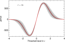
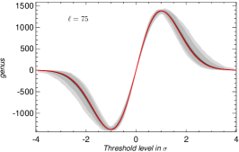
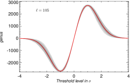
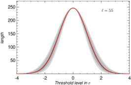
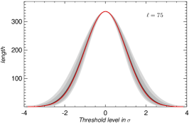
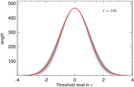
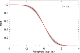
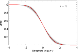
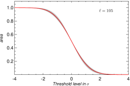
Figure 2: Multipole space Gaussian case: Analytical (red) vs simulations (black and grey). The legend shows the multipoles at which the LKCs are evaluated. Grey Shades are $68,95$ and $99\%$ percentiles estimated from 100 simulations.

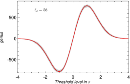
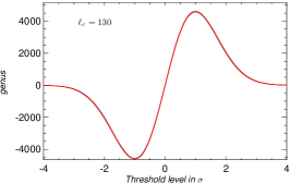
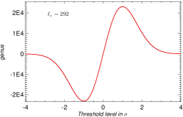
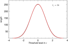
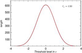
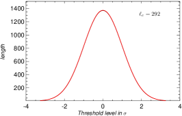
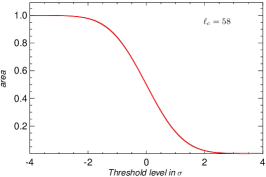
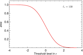
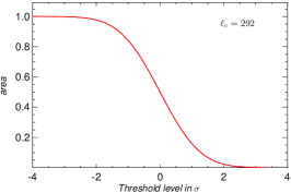
Figure 3: Needlet space Gaussian case: Analytical (red) vs simulations (black and grey). The needlet parameters are $B=1.5$ $j=10,12,14$. The central multipoles of the corresponding needlet filter is given in the legend. Grey Shades are $68,95$ and $99\%$ percentiles estimated from 100 simulations.

III NonGaussian expected values

Before we go ahead to discuss the analytic results, it is important to motivate the class of nonGaussian fields we wish to consider.

A major thread of last decade’s research in the field of CMB has been related to the investigation of possible asymmetries and directional variations in the observed data; seminal papers in this area were provided by Tegmark et al. (2003); Vielva et al. (2004); Eriksen et al. (2004a); Hansen et al. (2004); Park (2004); Land and Magueijo (2005); Larson and Wandelt (2004); Cruz et al. (2007); Copi et al. (2007) working on the early WMAP data release, but the field is still now very active and hotly debated, see Planck Collaboration et al. (2013) and the references therein. In this framework, it is well-known that needlet coefficients or fields can provide unbiased estimates for smoothed versions of the angular power spectrum, the bispectrum or any higher-order statistics; these estimates are spatially localized, so they can be immediately used to test for instance power asymmetries, an idea first developed in Baldi et al. (2009b), Pietrobon et al. (2008).

More explicitly, consider the squared field $\beta_{j}^{2}(x);$ from the localization properties of the needlet frame, it is obvious that the value of $\beta_{j}(x)$ is only determined by CMB radiation in a small neighbourhood around $x,$ while we have moreover

$$\mathbb{E}\beta_{j}^{2}(x)=\mathbb{E}\left\{\sum_{\ell=B^{j-1}}^{B^{j+1}}b^{2}(\frac{\ell}{B^{j}})T_{\ell}(x)\right\}^{2}=\sum_{\ell=B^{j-1}}^{B^{j+1}}b^{4}(\frac{\ell}{B^{j}})\frac{2\ell+1}{4\pi}C_{\ell}\text{ ,}$$

e.g., the squared coefficients provide natural unbiased estimates for a binned angular power spectrum. Along the same lines, the cube of these coefficients provides an unbiased, local estimator of the binned bispectrum, which is a natural candidate to search for directional variations in nonGaussianity:

$$\mathbb{E}\beta_{j}^{3}(x) = \mathbb{E}\left\{\sum_{\ell=B^{j-1}}^{B^{j+1}}b^{2}(\frac{\ell}{B^{j}})T_{\ell}(x)\right\}^{3}$$

$$= \sum_{\ell_{1},\ell_{2},\ell_{3}=B^{j-1}}^{B^{j+1}}b^{2}(\frac{\ell_{1}}{B^{j}})b^{2}(\frac{\ell_{2}}{B^{j}})b^{2}(\frac{\ell_{3}}{B^{j}})\mathbb{E}\left\{T_{\ell_{1}}(x)T_{\ell_{2}}(x)T_{\ell_{3}}(x)\right\}$$

$$= \sum_{\ell_{1},\ell_{2},\ell_{3}=B^{j-1}}^{B^{j+1}}b^{2}(\frac{\ell_{1}}{B^{j}})b^{2}(\frac{\ell_{2}}{B^{j}})b^{2}(\frac{\ell_{3}}{B^{j}})\left(\begin{array}[]{ccc}\ell_{1}&\ell_{2}&\ell_{3}\\ 0&0&0\end{array}\right)^{2}$$

$$\times b_{\ell_{1}\ell_{2}\ell_{3}}\sqrt{\frac{(2\ell_{1}+1)(2\ell_{2}+1)(2\ell_{3}+1)}{4\pi}}\text{ ,}$$

where $b_{\ell_{1}\ell_{2}\ell_{3}}$ denotes as usual the reduced bispectrum and the Wigner’s 3j symbols have appeared in the last equation, see Lan and Marinucci (2008), Donzelli et al. (2012) for more references and details. In the remaining part of this Section we shall provide the analytic expectation also for the Minkowski functionals/Lipschitz-Killing curvatures of these cubic statistics. These results can be rigorously derived by an application of a more general form of the Gaussian Kinematic formula, which is given in the Appendix. However, from a more heuristic point of view their derivation can be provided from a very simple argument. Indeed, consider for instance a quadratic transformed field $W=T^{2}:$ the excursion region of the field $W$ over a level $u$ is easily seen to be given by the region where $T>\sqrt{u},$ plus the region where $T<-\sqrt{u}.$ In view of the decoupling we reported below, the expected values of the LKCs for the quadratic case turn out to be just the sum of the corresponding Gaussian results over these two regions. Likewise, for the cubic case $W=T^{3}$ the excursion region will be obtained by simply considering the excursion sets of $T$ over the level $\sqrt[3]{u}.$ This simple heuristic would not work in more complicated circumstances where the GKF still provides exact solutions, but it is enough to justify the results we report below.

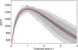
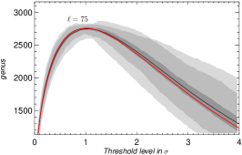
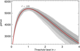
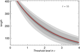
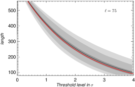
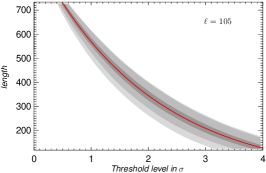
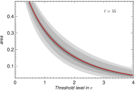
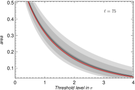
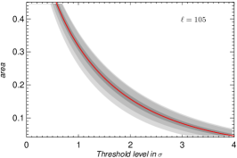
Figure 4: Multipole space nonGaussian quadratic case: Analytical (red) vs simulations (black and grey). The legend shows the multipoles at which the LKCs are evaluated. Grey Shades are $68,95$ and $99\%$ percentiles estimated from 100 simulations.

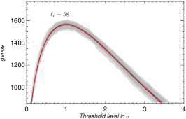
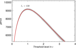
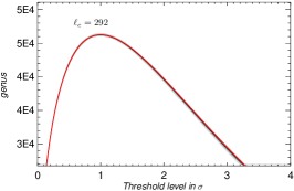
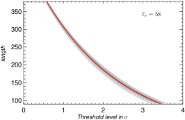
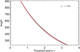
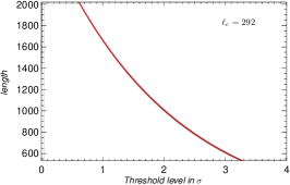
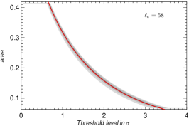
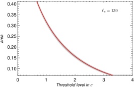
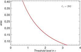
Figure 5: Needlet space nonGaussian quadratic case: Analytical (red) vs simulations (black and grey). The needlet parameters are $B=1.5$ $j=10,12,14$. The central multipoles of the corresponding needlet filter is given in the legend. Grey Shades are $68,95$ and $99\%$ percentiles estimated from 100 simulations.

III.1 The Quadratic case

We start from the case where we square the needlet field, as if we were interested in local estimates of the power spectrum. As usual, we normalize the starting Gaussian field to have unit variance, and we are hence focusing on the square field defined by

$$\beta_{j,2}(x)=\frac{\beta_{j}^{2}(x)}{Var(\beta_{j}(x))}=\frac{\beta_{j}^{2}(x)}{\sum_{\ell}b^{4}(\frac{\ell}{B^{j}})\frac{2\ell+1}{4\pi}C_{\ell}}\text{ .}$$

As motivated by the previous heuristic, or as derived more rigorously by the general Gaussian kinematic formula (see Appendix), we have the following analytic predictions:

• For the expected value of the Euler characteristic

  $$\mathbb{E}\mathcal{L}_{0}(A_{u})=4(1-\Phi(\sqrt{u}))+4\frac{\sum_{\ell}b^{4}(\frac{\ell}{B^{j}})\frac{2\ell+1}{4\pi}C_{\ell}\frac{\ell(\ell+1)}{2}}{\sum_{\ell}b^{4}(\frac{\ell}{B^{j}})\frac{2\ell+1}{4\pi}C_{\ell}}\frac{e^{-u/2}}{\sqrt{2\pi}}\sqrt{u}\text{ ;}$$

• For the second Lipschitz-Killing curvature (i.e., half of the boundary length)

  $$\mathbb{E}\mathcal{L}_{1}(A_{u})=2\pi\left\{\frac{\sum_{\ell}b^{4}(\frac{\ell}{B^{j}})\frac{2\ell+1}{4\pi}C_{\ell}\frac{\ell(\ell+1)}{2})}{\sum_{\ell}b^{4}(\frac{\ell}{B^{j}})\frac{2\ell+1}{4\pi}C_{\ell}}\right\}^{1/2}e^{-u/2}\text{ ;}$$

• Finally for the area of excursion regions

  $$\mathbb{E}\mathcal{L}_{2}(A_{u})=4\pi\times 2(1-\Phi(\sqrt{u}))\text{ .}$$

The results for the square of normalized multipole components ($T_{\ell}^{2}/\mathbb{E(}T_{\ell}^{2}))$ are entirely analogous, indeed even simpler to state:

• For the expected value of the Euler characteristic

  $$\mathbb{E}\mathcal{L}_{0}(A_{u})=4(1-\Phi(\sqrt{u}))+4\frac{\ell(\ell+1)}{2}\frac{e^{-u/2}}{\sqrt{2\pi}}\sqrt{u}\text{ ;}$$

• For the second Lipschitz-Killing curvature (i.e., half of the boundary length)

  $$\mathbb{E}\mathcal{L}_{1}(A_{u})=2\pi\left\{\frac{\ell(\ell+1)}{2}\right\}^{1/2}e^{-u/2}\text{ ;}$$

• Finally for the area of excursion regions

  $$\mathbb{E}\mathcal{L}_{2}(A_{u})=4\pi\times 2(1-\Phi(\sqrt{u}))\text{ .}$$

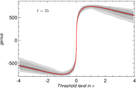
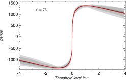
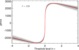
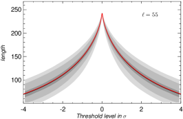
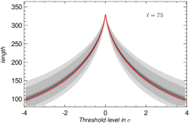
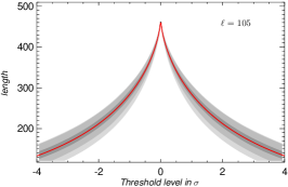
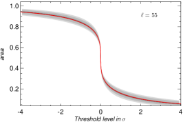
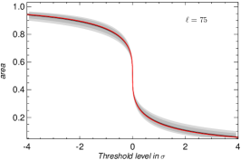
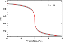
Figure 6: Multipole space nonGaussian cubic case: Analytical (red) vs simulations (black and grey). The legend shows the multipoles at which the LKCs are evaluated. Grey Shades are $68,95$ and $99\%$ percentiles estimated from 100 simulations.

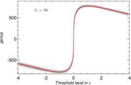
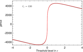
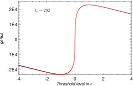
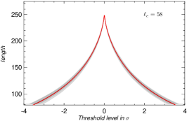
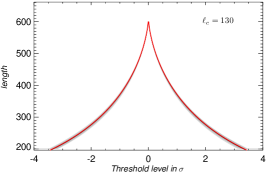
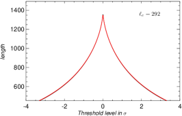
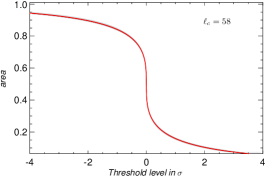
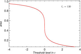
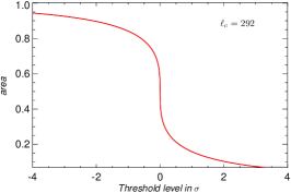
Figure 7: Needlet space nonGaussian cubic case: Analytical (red) vs simulations (black and grey). The needlet parameters are $B=1.5$ $j=10,12,14$. The central multipoles of the corresponding needlet filter is given in the legend. Grey Shades are $68,95$ and $99\%$ percentiles estimated from 100 simulations.

III.2 The cubic case $\beta_{j}^{3}(x)$

Cubic transformations are the natural candidates to search for anisotropies in the bispectrum, are at least in the skewness; we simply take the cube of the needlet fields. The analytic prediction are then as follows (see also Marinucci and Vadlamani (2013) and the Appendix for details):

• The expected value of the Euler characteristic is given by

  $$\mathbb{E}\mathcal{L}_{0}(A_{u}(\beta_{j}^{3}(x);S^{2}))=2(1-\Phi(\sqrt[3]{u}))+2\frac{\sum_{\ell}b^{4}(\frac{\ell}{B^{j}})\frac{2\ell+1}{4\pi}C_{\ell}\frac{\ell(\ell+1)}{2}}{\sum_{\ell}b^{4}(\frac{\ell}{B^{j}})\frac{2\ell+1}{4\pi}C_{\ell}}\frac{e^{-(\sqrt[3]{u})^{2}/2}}{\sqrt{2\pi}}\sqrt[3]{u}\text{ ;}$$

• The expected value for half the boundary length is

  $$\mathbb{E}\mathcal{L}_{1}(A_{u}(\beta_{j}^{3}(x);S^{2}))=\pi\left\{\frac{\sum_{l}b^{4}(\frac{\ell}{B^{j}})\frac{2\ell+1}{4\pi}C_{\ell}\frac{\ell(\ell+1)}{2}}{\sum_{\ell}b^{4}(\frac{\ell}{B^{j}})\frac{2\ell+1}{4\pi}C_{\ell}}\right\}^{1/2}e^{-(\sqrt[3]{u})^{2}/2}\text{ ;}$$

• Finally, the expected value of the area of excursion regions is

  $$\mathbb{E}\mathcal{L}_{2}(A_{u}(\beta_{j}^{3}(x);S^{2}))=4\pi(1-\Phi(\sqrt[3]{u}))\text{ .}$$

The corresponding values for the cube of normalized multipole components are given by

• The expected value of the Euler characteristic is given by

  $$\mathbb{E}\mathcal{L}_{0}(A_{u}(\beta_{j}^{3}(x);S^{2}))=2(1-\Phi(\sqrt[3]{u}))+2\frac{\ell(\ell+1)}{2}\frac{e^{-(\sqrt[3]{u})^{2}/2}}{\sqrt{2\pi}}\sqrt[3]{u}\text{ ;}$$

• The expected value for half the boundary length is

  $$\mathbb{E}\mathcal{L}_{1}(A_{u}(\beta_{j}^{3}(x);S^{2}))=\pi\left\{\frac{\ell(\ell+1)}{2}\right\}^{1/2}e^{-(\sqrt[3]{u})^{2}/2}\text{ ;}$$

• Finally, the expected value of the area of excursion regions is

  $$\mathbb{E}\mathcal{L}_{2}(A_{u}(\beta_{j}^{3}(x);S^{2}))=4\pi(1-\Phi(\sqrt[3]{u}))\text{ .}$$

It should be noted that the area measure is completely insensitive to the behaviour of the correlation structure, and therefore takes the same values in the needlet and multipole cases.

We recall that in Marinucci and Vadlamani (2013) further nonGaussian cases have been considered, e.g. the situation where the polynomial transforms of these coefficients are further averaged by moving disks centred at varying pixels on the sphere. Analytical results have been provided even for these circumstances, however for brevity’s sake we delay their investigation to future research.

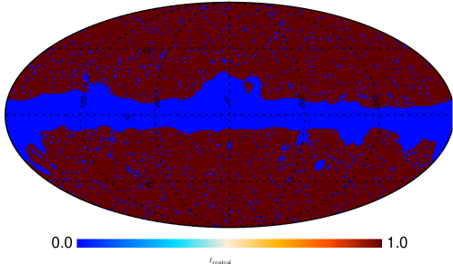
Figure 8: Planck Union mask. The fractional area of the unmasked region is $f_{sky}=0.73$.

IV Masked Regions

In the analysis of data collected from experiments with masked regions, as it is basically always the case in Cosmology, the full power of the GKF emerges most clearly. Let us denote by $M=S^{2}\backslash G$ the sphere to which the masked regions (for instance, the galactic cut) have been subtracted; it is then sufficient to replace the LKCs $\mathcal{L}_{i+l}(M)$ to $\mathcal{L}_{i+l}(S^{2})$ in (3),(4) to obtain the desired result. At first sight, however, this may appear as a very difficult task; how to replace the simple values provided in (4) with the LKC for a masked region, possibly with a highly complicated structure including many removed point sources and other foreground regions with complex shapes? For the area measure $\mathcal{L}_{2}(S^{2}\backslash G)$ the computation could be trivial (by simply adjusting the sky fraction), but for the boundary length $\mathcal{L}_{1}(S^{2}\backslash G)$ and the Euler-Poincaré characteristic $\mathcal{L}_{0}(S^{2}\backslash G)$ this problem may seem quite hard, especially when a huge number of removed point sources is given.

A very simple solution can however be provided by exploiting one more time Gaussian Kinematic Formula, following an idea discussed in Adler and Taylor (2011), chapter 5.4. In fact, for any given mask one can choose a simple isotropic random field with known angular power spectrum, and from this one may evaluate by Monte Carlo simulations the realized values of LKC of excursion sets at some fixed levels of threshold values $u$. These realized values can then be compared with the analytic predictions; for a given input angular power spectrum, these are fully known, up to some fixed parameters representing the LKCs $\mathcal{L}_{i}(S^{2}\backslash G)$. These parameters can then be estimated once for all by simple least square regression, and used as an input to derive analytic predictions for a given mask. These predictions would hold for arbitrary threshold values $u$ and irrespective of the covariance structure, the frequency or scales $j,\ell$ considered, the Gaussian or nonGaussian circumstances.

In summary, the following multi-step procedure is advocated:

1. Fix a simple power spectrum $C_{\ell},$ for instance with $L_{\max}=10,$ and generate Gaussian maps out of it

2. Fix a limited number of threshold values $u$ and perform a Monte Carlo evaluation of the LKCs evaluated on the excursion set of the fields generated according to 1

3. Use least square regression to estimate $\mathcal{L}_{i}(S^{2}\backslash G)$, $i=0,1,2$ in equation (3)

4. Use the estimates obtained in point 3 as an input for equation (3) for any arbitrary power spectrum (for instance, multipole or needlet components on realizations of a $\Lambda CDM$ model, under Gaussian and nonGaussian circumstances).

We believe that this routine illustrates very vividly the advantages of the decoupling between domain manifold, covariance structure and threshold value achieved by the Gaussian Kinematic Formula (3). The resulting predictions are indeed extremely accurate, as illustrated in the following Section.

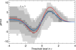
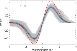
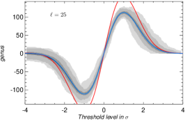
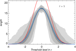
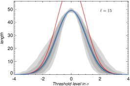
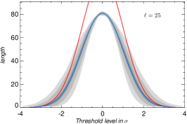
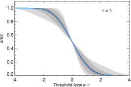
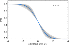
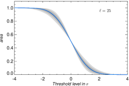
Figure 9: Multipole space Gaussian masked case: Analytical (red - full sky; blue - mask corrected) vs simulations (black and grey). The legend shows the multipoles at which the LKCs are evaluated. Grey Shades are $68,95$ and $99\%$ percentiles estimated from 100 simulations.

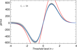
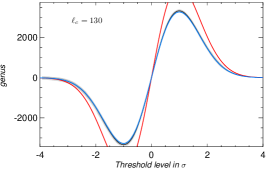
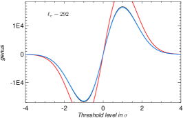
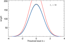
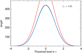
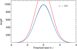
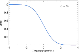
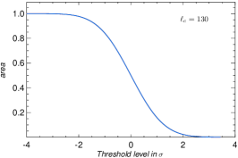
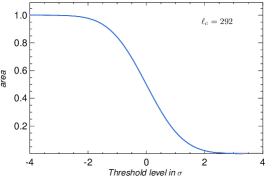
Figure 10: Needlet space nonGaussian masked case: Analytical (red - full sky; blue - mask corrected) vs simulations (black and grey). The needlet parameters are $B=1.5$ $j=10,12,14$. The central multipoles of the corresponding needlet filter is given in the legend. Grey Shades are $68,95$ and $99\%$ percentiles estimated from 100 simulations.

V Numerical results

In this section we describe the comparison of the analytical results outlined in the previous sections to the corresponding results from simulations. In all cases we generated 100 map realizations of an input power spectrum using the HEALpix Górski et al. (2005) package. We estimated LKCs from each simulations and compared their mean with the analytical results. We found an excellent agreement in all the cases that we investigated; more precisely, not only the estimated curves are always well within the $68\%$ Confidence Interval (CL), but actually as shown below they are for practical purposes basically indistinguishable from the theoretical predictions even with a relatively low number of Monte Carlo simulations.

Simulations and Algorithm

We used HEALpix synfast to simulate a map from a given power spectrum; the choice of this power spectrum has no influence on the results we shall provide. The procedures to obtain the single multipole or needlet maps are standard and can be described as follows: first we harmonic transform the simulated maps using anafast; then to obtain $T_{\ell}(x)$ or $\beta_{j}(x)$ maps, we simply take the appropriate inverse transform across the relevant multipoles, in the case of needlets inserting also the squared needlet filter $b^{2}(.)$. The multipole/needlet maps are then normalized by their root mean square, which is computed analytically using the input power spectrum, see below.

From these normalized multipole/needlet maps we then computed the three Minkowski Functionals, which as argued earlier are equivalent to the LKCs up to constant factors. This implementation is achieved exploiting the algorithms described in Eriksen et al. (2004b). In short, these algorithms can be described as follows: the area, i.e. the first MF, is computed by evaluating the number of pixels above a certain threshold. The length, the second MF, is computed by tracing isocontour lines in pixel space. For a sufficiently high-resolution map, pixels around isocontour lines have different signs relative to the contour line, after normalizing the lines to zero. To measure the length of these lines, sets of four pixels are compared; when at least two of them have different signs, the locations where the contour line enters and exits these sets of pixels are determined and the length is iteratively calculated by standard dot product. The Euler-Poincareé, the third MF, is computed by means of its characterizations through Morse theory; more explicitly, critical points are determined as the pixels where the gradient vanishes. The Hessian matrices around these critical points are computed, and their so-called indexes (i.e., the sign of their determinant, or the product of their eigenvalues) are evaluated. Positive indexes correspond to extrema (minima plus maxima), negative indexes to saddles; in two dimensions, the Euler-Poincaré characteristic is simply obtained as the difference between the number of extrema and the number of saddles.

On normalization issues

As mentioned, all the maps we used to estimate the LKCs are normalized to have unit variance; hence the threshold levels $-2,-1,0,1,2,\dots$ are given in terms of the standard deviation. It should be noted that at low multipoles, the sample variance need not be close to the population value, due to Cosmic Variance effect. As a result of this, normalizing maps by their respective sample root mean square would lead to incorrect estimates of the mean and variance of LKCs. We also stress that population variances can trivially be derived from any given power spectrum; for instance, the variance of a needlet map at frequency $j$ is given by

$$\sigma^{2}(\beta_{j})=\sum_{\ell=B^{j-1}}^{B^{j-1}}{b^{4}(\frac{\ell}{B^{j}})\frac{(2\ell+1)C_{l}}{4\pi}}$$

In the case where the input spectra are not known, one should use the best-fit power spectra from the map to compute the normalization factor.

Code validation

To understand the accuracy of our code in estimating the MFs, in particular in measuring the length of isocontour lines, we used some test functions for which the relevant quantities are analytically known. For instance one such function we used is

$$f(\theta,\phi)=sin(n\theta),$$

for which the length of isocontour lines at level zero are given by $2\pi\sum_{k=1}^{n-1}sin(\frac{k}{n}\pi)$; the results from our code are consistent with these theoretical values to better than $0.001\%$. Of course, the accuracy may degrade for highly oscillatory functions, but we believe this test provides a good validation to the entire pipeline and shows that the algorithms we employed are very reliable.

Results: Gaussian fields

In Figure (2) we compare the multipole space analytical results (red curve) given in Section II.2 with that of the simulations (black curve - mean of the simulations). The $68\%,95\%$ and $99\%$ CLs are shown from dark to light grey bounds. From left to right panels, the plots shows the results corresponding to multipoles $\ell=5,50,105$. We stress that our fit is extremely accurate, even at very low multipole values where the flat-sky approximation which is usually adopted cannot be expected to hold. We also note the improved concentration around the expected values at higher-multipoles; indeed, the same behaviour of these variances can be predicted analytically, but we delay these results for future work.

Likewise, Figure (3) shows analogous results in needlet space; the colors for different curves have the same meaning as described above. The displayed results cover the frequencies $j=10,12,14$ which for $B=1.5$ correspond to multipoles in the order of 60,130,200; these results are even more accurate than in the multipole case, in particular the decay of Cosmic Variance is faster.

Results: Non-Gaussian fields

As described before, our non-Gaussian maps are constructed by taking a power transform of a Gaussian input. We also argued earlier in Section III that the quadratic power transform seems useful to investigate power spectrum asymmetries, while the cubic transform provides a natural probe of possible directional variations in non-Gaussianity.

In Figure (4) and Figure (5) we compare the analytical results for the quadratic case in multipole and needlet space with those from the simulations, respectively. As described above the red curves are for analytical predictions, while the black and grey ones are for simulations.

Similarly, in Figure (6) and Figure (7) we show analytical vs. simulation results for the cubic nonGaussian case in multipole and needlet space, respectively. The fit between predicted values and simulations is again extremely good.

Results: masked sky case

Probably the main contribution in this paper relates to the possibility to use the GKF to handle analytically the effect of sky cuts on Minkowski functionals, see the discussion in Section IV. As a numerical validation of the analytical results for the expected values of LKCs in the presence of sky-mask, here we use the realistic Planck official sky mask, which is formed as a union of different foreground separation methods confidence masks together with point source masks. The cut regions are shown in Figure (8), leaving on observed area of $f_{\rm sky}=73\%$. As explained earlier, the key step is the evaluation of LKCs for the masked sphere, which can then be used as input values to predict the LKCs of excursion sets under arbitrary covariance structures. In particular, the input LKCs for the masked sphere have been derived by simulation from a masked single multipole field at $\ell=15$, map; this ensures that the estimation procedure can be implemented with remarkable computational efficiency. The resulting values are then inserted to obtain the analytic predictions at any frequency or multipole.

In Figure (9) and Figure (10) we compare the masked Gaussian field analytical result with the corresponding simulations in multipole and needlet space, respectively. Of course, here as for the other cases the most relevant results in practice are those for needlets, because single multipoles cannot be extracted from masked data; nevertheless, it is reassuring that the fit works in both circumstances. Moreover, the analysis of multipole components can be exploited to verify the statistical properties of full-sky maps, as those obtained for instance by means of inpainting techniques. These issues are left as topics for further research.

VI Summary and Conclusion

In this paper, we illustrated a number of applications for Cosmological data analysis of the Gaussian Kinematic Formula (GKF), (see Taylor and Adler (2003); Taylor (2006); Adler et al. (2009), Adler and Taylor (2011), Adler and Taylor (2007)). The Gaussian Kinematic Formula allows to evaluate exact expected values for Lipschitz-Killing curvatures (Minkowski functionals) in a number of circumstances of applied interest, covering in particular full-sky experiments (accounting for the geometry of the sphere), nonlinear statistics and masked data.

We used the GKF on random fields derived by harmonic and needlet transforms, allowing for the further advantage of better control of Cosmic Variance effects and localization. In particular we provided the analytic expressions for the Minkowski functionals for needlets and single multipole fields, covering Gaussian and nonGaussian circumstances, with and without masks. All the results reported are validated by an extensive Monte Carlo study, which demonstrates an extremely good agreement between predictions and simulations.

VII Acknowledgments

The authors acknowledge support from ERC Grant 277742 Pascal. We acknowledge the use of resources from the Norwegian national super-computing facilities, NOTUR. Maps and results have been derived using the HEALpix (http://healpix.jpl.nasa.gov) software package developed by Górski et al. (2005).

VIII Mathematical Appendix

On a general, high-dimensional manifold, the LKCs for the region $A$ are defined as the coefficients of a Taylor expansion of a Tube of radius $r$ around $A.$ Formally, a Tube is simply the set $A$ plus an halo, i.e.

$$Tube(A,r)=\left\{x:d(x,A)\leq r\right\}\text{ .}$$

assuming that $A$ had dimension $\dim(A)=n,$ the LKCs are implicitly defined by the formula

$$Vol\left[Tube(A,r)\right]=\sum_{k=0}^{n}\mathcal{L}_{n-k}(A)\omega_{k}r^{k}.$$

For instance, let $A$ be the unit square on the plane; by elementary geometry, the volume of the Tube is then given by

$$\mathcal{L}_{2}(A)+2\mathcal{L}_{1}(A)r+\mathcal{L}_{0}(A)\pi r^{2}=1+2\cdot 2\cdot r+\pi r^{2},$$

whence it is seen that in the two-dimensional case the LKCs correspond to Euler-Poincaré characteristic, half the boundary length and area, respectively. This definition extends to arbitrary manifolds and dimensions, and makes it possible to express the GKF in much greater generality. Similarly, one can introduce the Gaussian Minkowski functionals $\mathcal{M}_{k}(U)$ as the Taylor coefficients in the expansion of the Tube probabilities, e.g

$$\Pr\left\{Z\in Tube(U,r)\right\}=\sum_{k}\mathcal{M}_{k}(U)\frac{r^{k}}{k!}.$$

The left-hand side simply represents the probability that a zero-mean standard Gaussian variable belongs to $Tube(U,r);$ for instance, for $U=[u,\infty)$ it can be checked that the Gaussian Minkowski functionals yield the $k-$order derivatives of Gaussian densities that we recalled above. More general forms of $U$ are necessary, however, when one considers nonGaussian processes, as we shall do below.

We shall now discuss the Gaussian kinematic formula for the case of nonlinear transforms of Gaussian and isotropic random fields; i.e., we shall consider fields of the form

$$y(x)=g(T(x))\text{ , }$$

where $T(x)$ is zero-mean, unit variance, Gaussian and isotropic, and the function $g(.)$ is such that also $y(.)$ has finite variance; for our purposes, the examples we shall consider are simply quadratic and cubic polynomials, i.e. $g(T)=T^{2}$ and $g(T)=T^{3}.$ Under these circumstances, the Gaussian kinematic formula takes the form

$$\lambda^{i/2}\mathbb{E}\mathcal{L}_{i}(A_{u}(g(T),M))=\sum_{k=0}^{\dim(M)-i}\lambda^{(i+k)/2}\mathcal{L}_{i+k}(M)\mathcal{M}_{k}(g^{-1}[u,\infty))\text{ ;}$$ (13)

the expression obviously becomes identical to (3), in the Gaussian case $g(T(x))=T(x).$ For more general transforms, the role of the Gaussian Minkowski functionals becomes crucial: these are rather simple to evaluate for quadratic and cubic cases, as we shall show below.

VIII.1 The Quadratic Case

Here we are interested in the analysis of quadratic functionals such as

$$g(\beta_{j}(x))=\frac{\beta_{j}^{2}(x)}{\mathbb{E}\beta_{j}^{2}(x)}\text{ .}$$

By the general Gaussian kinematic formula and simple computations we have

$$\mathbb{E}\mathcal{L}_{0}(A_{u}(g(\beta_{j}(x)),S^{2}) = \sum_{k=0}^{2}(2\pi)^{-k/2}\lambda_{j}^{k/2}\mathcal{L}_{k}(S^{2})\mathcal{M}_{k}((-\infty,-\sqrt{u})\cup(\sqrt{u},\infty))$$

$$= \sum_{k=0}^{2}(2\pi)^{-k/2}\lambda_{j}^{k/2}\mathcal{L}_{k}(S^{2})2\mathcal{M}_{k}^{\mathcal{N}}((\sqrt{u},\infty))$$

$$=2\cdot 2\cdot(1-\Phi(\sqrt{u}))+0+\frac{1}{2\pi}\mathcal{L}_{2}^{\beta_{j}}(S^{2})\frac{e^{-u/2}}{\sqrt{2\pi}}2\sqrt{u}$$

$$=2\cdot 2\cdot(1-\Phi(\sqrt{u}))+\frac{1}{2\pi}\frac{\sum_{\ell}b^{2}(\frac{\ell}{B^{j}})\frac{2\ell+1}{4\pi}C_{\ell}\frac{\ell(\ell+1)}{2}}{\sum_{\ell}b^{2}(\frac{\ell}{B^{j}})\frac{2\ell+1}{4\pi}C_{\ell}}\mathcal{L}_{2}(S^{2})\frac{e^{-u/2}}{\sqrt{2\pi}}2\sqrt{u}\text{ .}$$

Also

$$\lambda_{j}^{1/2}\mathbb{E}\mathcal{L}_{1}((A_{u}(g(\beta_{j}(x)),S^{2})) = \sum_{k=0}^{1}(2\pi)^{-k/2}\left[\begin{array}[]{c}k+1\\ k\end{array}\right]\lambda_{j}^{(k+1)/2}\mathcal{L}_{k+1}(S^{2})\mathcal{M}_{k}(g^{-1}[u,\infty))$$

$$= \lambda_{j}^{1/2}\mathcal{L}_{1}(S^{2})\mathcal{M}_{0}((-\infty,-\sqrt{u})\cup(\sqrt{u},\infty))$$

$$+(2\pi)^{-1/2}\frac{\pi}{2}\lambda_{j}\mathcal{L}_{2}(S^{2})\mathcal{M}_{1}^{\mathcal{N}}((-\infty,-\sqrt{u})\cup(\sqrt{u},\infty))$$

$$= (2\pi)^{-1/2}\frac{\pi}{2}(4\pi\frac{\sum_{\ell}b^{2}(\frac{\ell}{B^{j}})\frac{2\ell+1}{4\pi}C_{\ell}\frac{\ell(\ell+1)}{2}}{\sum_{\ell}b^{2}(\frac{\ell}{B^{j}})\frac{2\ell+1}{4\pi}C_{\ell}}\mathcal{)}2\frac{e^{-u/2}}{\sqrt{2\pi}}$$

$$= 2\pi(\frac{\sum_{\ell}b^{2}(\frac{\ell}{B^{j}})\frac{2\ell+1}{4\pi}C_{\ell}\frac{\ell(\ell+1)}{2}}{\sum_{\ell}b^{2}(\frac{\ell}{B^{j}})\frac{2\ell+1}{4\pi}C_{\ell}}\mathcal{)}e^{-u/2},$$

which implies

$$\mathbb{E}\mathcal{L}_{1}((A_{u}(g(\beta_{j}(x)),S^{2}))=2\pi\left\{\frac{\sum_{\ell}b^{2}(\frac{\ell}{B^{j}})\frac{2\ell+1}{4\pi}C_{\ell}\frac{\ell(\ell+1)}{2}}{\sum_{\ell}b^{2}(\frac{\ell}{B^{j}})\frac{2\ell+1}{4\pi}C_{\ell}}\right\}^{1/2}e^{-u/2}$$

entailing a length of the boundary of excursion sets given by

$$2\pi\left\{\frac{\sum_{\ell}b^{2}(\frac{\ell}{B^{j}})\frac{2\ell+1}{4\pi}C_{\ell}\frac{\ell(\ell+1)}{2}}{\sum_{\ell}b^{2}(\frac{\ell}{B^{j}})\frac{2\ell+1}{4\pi}C_{\ell}}\right\}^{1/2}e^{-u/2}.$$

Finally

$$\lambda_{j}\mathbb{E}\mathcal{L}_{2}((A_{u}(g(\beta_{j}(x)),S^{2})) = \lambda_{j}\mathcal{L}_{2}(S^{2})\mathcal{M}_{0}(g^{-1}(u,\infty))$$

$$= 4\pi\left\{\frac{\sum_{\ell}b^{2}(\frac{\ell}{B^{j}})\frac{2\ell+1}{4\pi}C_{\ell}\frac{\ell(\ell+1)}{2}}{\sum_{\ell}b^{2}(\frac{\ell}{B^{j}})\frac{2\ell+1}{4\pi}C_{\ell}}\right\}2(1-\Phi(\sqrt{u}))$$

implying that

$$\mathbb{E}\mathcal{L}_{2}((A_{u}(g(\beta_{j}(x)),S^{2}))=4\pi\times 2(1-\Phi(\sqrt{u}))\text{ .}$$

VIII.2 The Cubic Case $g(x)=x^{3}$

Again by applying (13), we obtain for needlet components

$$\mathbb{E}\mathcal{L}_{0}(A_{u}(\beta_{j}^{3}(x);S^{2})) = \sum_{k=0}^{2}(2\pi)^{-k/2}\mathcal{L}_{k}(S^{2})\mathcal{M}_{k}^{\mathcal{N}}((\sqrt[3]{u},\infty))$$

$$= 2(1-\Phi(\sqrt[3]{u}))+2\frac{\sum_{\ell}b^{2}(\frac{\ell}{B^{j}})\frac{2\ell+1}{4\pi}C_{\ell}\frac{\ell(\ell+1)}{2}}{\sum_{\ell}b^{2}(\frac{\ell}{B^{j}})\frac{2\ell+1}{4\pi}C_{\ell}}\frac{e^{-(\sqrt[3]{u})^{2}/2}}{\sqrt{2\pi}}\sqrt[3]{u}\text{ ,}$$

and likewise

$$\mathbb{E}\mathcal{L}_{1}(A_{u}(\beta_{j}^{3}(x);S^{2}))=2\pi\left\{\frac{\sum_{\ell}b^{2}(\frac{\ell}{B^{j}})\frac{2\ell+1}{4\pi}C_{\ell}\frac{\ell(\ell+1)}{2}}{\sum_{\ell}b^{2}(\frac{\ell}{B^{j}})\frac{2\ell+1}{4\pi}C_{\ell}}\right\}^{1/2}e^{-(\sqrt[3]{u})^{2}/2}.$$

Finally

$$\mathbb{E}\mathcal{L}_{2}(A_{u}(\beta_{j}^{3}(x);S^{2}))=4\pi(1-\Phi(\sqrt[3]{u}))\text{ .}$$

References

- Tomita (1986) H. Tomita, Progress of Theoretical Physics 76, 952 (1986).
- Coles (1988) P. Coles, MNRAS 234, 509 (1988).
- Schmalzing and Buchert (1997) J. Schmalzing and T. Buchert, ApJ 482, L1 (1997), eprint astro-ph/9702130.
- Dolgov et al. (1999) A. D. Dolgov, A. G. Doroshkevich, D. I. Novikov, and I. D. Novikov, International Journal of Modern Physics D 8, 189 (1999), eprint astro-ph/9901399.
- Naselsky and Novikov (1998) P. D. Naselsky and D. I. Novikov, ApJ 507, 31 (1998), eprint astro-ph/9801285.
- Novikov et al. (2000) D. Novikov, J. Schmalzing, and V. F. Mukhanov, A&A 364, 17 (2000), eprint astro-ph/0006097.
- Schmalzing and Gorski (1998) J. Schmalzing and K. M. Gorski, MNRAS 297, 355 (1998), eprint astro-ph/9710185.
- Matsubara (2003) T. Matsubara, ApJ 584, 1 (2003).
- Komatsu et al. (2003) E. Komatsu, A. Kogut, M. R. Nolta, C. L. Bennett, M. Halpern, G. Hinshaw, N. Jarosik, M. Limon, S. S. Meyer, L. Page, et al., ApJS 148, 119 (2003), eprint astro-ph/0302223.
- Spergel et al. (2007) D. N. Spergel, R. Bean, O. Doré, M. R. Nolta, C. L. Bennett, J. Dunkley, G. Hinshaw, N. Jarosik, E. Komatsu, L. Page, et al., ApJS 170, 377 (2007), eprint astro-ph/0603449.
- Natoli et al. (2010) P. Natoli, G. de Troia, C. Hikage, E. Komatsu, M. Migliaccio, P. A. R. Ade, J. J. Bock, J. R. Bond, J. Borrill, A. Boscaleri, et al., MNRAS 408, 1658 (2010), eprint 0905.4301.
- Matsubara (2010) T. Matsubara, Phys. Rev. D 81, 083505 (2010), eprint 1001.2321.
- Ducout et al. (2013) A. Ducout, F. R. Bouchet, S. Colombi, D. Pogosyan, and S. Prunet, MNRAS 429, 2104 (2013), eprint 1209.1223.
- Pratten and Munshi (2012) G. Pratten and D. Munshi, MNRAS 423, 3209 (2012), eprint 1108.1985.
- Munshi et al. (2013) D. Munshi, J. Smidt, A. Cooray, A. Renzi, A. Heavens, and P. Coles, MNRAS 434, 2830 (2013), eprint 1011.5224.
- Planck Collaboration et al. (2013) Planck Collaboration, P. A. R. Ade, N. Aghanim, C. Armitage-Caplan, M. Arnaud, M. Ashdown, F. Atrio-Barandela, J. Aumont, C. Baccigalupi, A. J. Banday, et al., ArXiv e-prints (2013), eprint 1303.5083.
- Adler (1981) R. J. Adler, The Geometry of Random Fields (Wiley Series in Probability and Statistics) (John Wiley & Sons Inc, 1981), ISBN 0471278440, URL http://www.worldcat.org/isbn/0471278440.
- Taylor and Adler (2003) J. E. Taylor and R. J. Adler, The Annals of Probability 31, 533 (2003), URL http://dx.doi.org/10.1214/aop/1048516527.
- Taylor (2006) J. E. Taylor, The Annals of Probability 34, 122 (2006), URL http://dx.doi.org/10.1214/009117905000000594.
- Adler et al. (2009) R. Adler, J. Ewing, and P. Taylor, Statistical Science 24, 1 (2009), URL http://dx.doi.org/10.1214/09-STS285.
- Adler and Taylor (2011) R. J. Adler and J. E. Taylor, Topological Complexity of Smooth Random Functions (Springer Berlin Heidelberg, 2011), ISBN 978-3-642-19579-2 (Print) 978-3-642-19580-8 (Online), URL http://www.springer.com/mathematics/probability/book/978-0-387-48112-8.
- Adler and Taylor (2007) R. J. Adler and J. E. Taylor, Random Fields and Geometry (Springer New York, 2007), ISBN 9780387481128, URL http://www.springer.com/mathematics/geometry/book/978-3-642-19579-2.
- Bobin et al. (2014) J. Bobin, F. Sureau, J.-L. Starck, A. Rassat, and P. Paykari, A&A 563, A105 (2014), eprint 1401.6016.
- Górski et al. (2005) K. M. Górski, E. Hivon, A. J. Banday, B. D. Wandelt, F. K. Hansen, M. Reinecke, and M. Bartelmann, ApJ 622, 759 (2005), eprint astro-ph/0409513.
- Narcowich et al. (2006) F. J. Narcowich, P. Petrushev, and J. D. Ward, SIAM J. Math. Anal p. 2237162 (2006).
- Baldi et al. (2009a) P. Baldi, G. Kerkyacharian, D. Marinucci, and D. Picard, The Annals of Statistics 37, 1150 (2009a), URL http://dx.doi.org/10.1214/08-AOS601.
- Marinucci et al. (2008) D. Marinucci, D. Pietrobon, A. Balbi, P. Baldi, P. Cabella, G. Kerkyacharian, P. Natoli, D. Picard, and N. Vittorio, MNRAS 383, 539 (2008), eprint 0707.0844.
- Donzelli et al. (2012) S. Donzelli, F. K. Hansen, M. Liguori, D. Marinucci, and S. Matarrese, ApJ 755, 19 (2012), eprint 1202.1478.
- Marinucci and Vadlamani (2013) D. Marinucci and S. Vadlamani, ArXiv e-prints (2013), eprint 1303.2456.
- Tegmark et al. (2003) M. Tegmark, A. de Oliveira-Costa, and A. Hamilton, Phys.Rev. D68, 123523 (2003), eprint astro-ph/0302496.
- Vielva et al. (2004) P. Vielva, E. Martinez-Gonzalez, R. Barreiro, J. Sanz, and L. Cayon, Astrophys.J. 609, 22 (2004), eprint astro-ph/0310273.
- Eriksen et al. (2004a) H. K. Eriksen, F. K. Hansen, A. J. Banday, K. M. Gorski, and P. B. Lilje, ApJ 605, 14 (2004a), eprint arXiv:astro-ph/0307507.
- Hansen et al. (2004) F. K. Hansen, A. J. Banday, and K. M. Górski, MNRAS 354, 641 (2004), eprint arXiv:astro-ph/0404206.
- Park (2004) C. G. Park, MNRAS 349, 313 (2004).
- Land and Magueijo (2005) K. Land and J. Magueijo, Phys.Rev.Lett. 95, 071301 (2005), eprint astro-ph/0502237.
- Larson and Wandelt (2004) D. L. Larson and B. D. Wandelt, Astrophys.J. 613, L85 (2004), eprint astro-ph/0404037.
- Cruz et al. (2007) M. Cruz, L. Cayon, E. Martinez-Gonzalez, P. Vielva, and J. Jin, Astrophys.J. 655, 11 (2007), eprint astro-ph/0603859.
- Copi et al. (2007) C. Copi, D. Huterer, D. Schwarz, and G. Starkman, Phys.Rev. D75, 023507 (2007), eprint astro-ph/0605135.
- Baldi et al. (2009b) P. Baldi, G. Kerkyacharian, D. Marinucci, and D. Picard, Bernoulli 15, 438 (2009b), URL http://dx.doi.org/10.3150/08-BEJ164.
- Pietrobon et al. (2008) D. Pietrobon, A. Amblard, A. Balbi, P. Cabella, A. Cooray, et al., Phys.Rev. D78, 103504 (2008), eprint 0809.0010.
- Lan and Marinucci (2008) X. Lan and D. Marinucci, Electronic Journal of Statistics 2, 332 (2008), eprint 0802.4020.
- Eriksen et al. (2004b) H. K. Eriksen, D. I. Novikov, P. B. Lilje, A. J. Banday, and K. M. Górski, ApJ 612, 64 (2004b), eprint astro-ph/0401276.