On the alternative formulation of the three-dimensional noncommutative superspace

Abstract

In this paper we propose a new version for the noncommutative superspace in 3D. This version is shown to be convenient for performing quantum calculations. In the paper, we use the theory of the chiral superfield as a prototype for possible generalizations, calculating the one-loop two-point function of a chiral supefield and the one-loop low-energy effective action in this theory.

The superspace, with no doubts, is a key idea of the supersymmetry concept. By its essence Superspace , the superspace is an extension of the usual Minkowski spacetime involving additional fermionic coordinates. Within the traditional supersymmetry, these extra coordinates obey the Grassmannian anticommutation relations, and the superfields are introduced as functions on the superspace. Further, all well-developed methodology of quantum field theories can be directly generalized for the superfields which allowed to elaborate supersymmetric extensions for the scalar field theories, gauge theories and gravity, and to study the properties of these supersymmetric theories on a quantum level.

The important step in the generalization of the superspace methodology was carried out in FL where the non(anti)commutativity for the fermionic coordinates was proposed. Further, the concept of the noncommutative superspace was formulated in a closed form in KPT . Following it, one should suggest that the fermionic superspace coordinates obey the Clifford anticommutation relations instead of the Grassmann ones. It was showed in KPT that this formulation can be developed only by paying a price of a partial supersymmetry breaking. As a consequence, the non-anticommutative deformation of ${\cal N}=1$ supersymmetric theory implies a theory with ${\cal N}=\frac{1}{2}$ supersymmetry Sei . One can note that, from a formal viewpoint, introduction of the Clifford anticommutation relations, involving the constant symmetric matrix, implements some special form of the Lorentz symmetry breaking in supersymmetric field theories different from the Berger-Kostelecky approach BK where the deformation of the supersymmetry algebra is introduced in other way. At the same time, the Clifford anticommutation relations naturally imply formulating the Moyal product for the superfield, which, however, unlike the usual Moyal product, contains only a finite number of terms. Among the important features of this approach, one should also mention that the formulation of the noncommutative superspace is, first, essentially based on chiral representation of the supersymmetry algebra, second, is consistent only in the Euclidean space KPT .

Further, the formalism of ${\cal N}=\frac{1}{2}$ supersymmetry was successfully applied for formulation of superfield models on the noncommutative superspace Sei and shown to possess some deep motivations from the superstring theory BerSe . Afterwards, the perturbative methodology was successfully applied for different ${\cal N}=\frac{1}{2}$ supersymmetric theories such as the ${\cal N}=\frac{1}{2}$ Wess-Zumino model whose renormalization properties have been discussed in NCWZ ; NCWZ1 ; Spurion , ${\cal N}=\frac{1}{2}$ supersymmetric gauge theories whose formulation and renormalizability have been studied in Penati ; Penati1 (see also Ito ; Ito1 ; Ito2 ; Ito3 for discussions on this issue), and extended supersymmetric theories, in particular, those ones formulated in terms of the harmonic superspace FerrIv ; FerrIv1 . The calculation of the superfield effective potential for this kind of theories BBP ; BBP1 ; BBP2 ; BBP3 also deserves to be mentioned.

At the same time, the superspace formulation of the three-dimensional field theories is well defined Superspace . Therefore, the generalization of the concept of the noncommutative superspace for the three-dimensional case seems to be very natural and interesting. However, the natural problem arising in this study is well known earlier : while in the four-dimensional case one has two sets of supersymmetry generators $Q_{\alpha}$ and $\bar{Q}_{\dot{\alpha}}$, so, deformation of the anticommutation relation between the fermionic coordinates implies only a partial supersymmetry breaking, in the three-dimensional case such a deformation results in a complete supersymmetry breaking. It was suggested in earlier by some of us that a natural way to circumvent this difficulty would consist in using of the extended, ${\cal N}=2$ supersymmetric theories from the very beginning, with further this extended supersymmetry is partially broken. However, in earlier , as well as further in Faizal ; Faizal1 ; Faizal2 where some alternative ways to realize this idea have been proposed, only some studies at the classical level have been carried out. At the same time, the use of the formulation of ${\cal N}=2$ three-dimensional superspace proposed in Hitchin , and further applied for the quantum calculations in BS ; Buch1 ; BMS and earlierHD , seems to be much more advantageous for development of the noncommutative superspace approach, due to the similarity of the ${\cal N}=2$ supersymmetry algebra in three-dimensional theories within this formulation and the ${\cal N}=1$ supersymmetry algebra in the four-dimensional theories. Therefore, in this paper we formulate the noncommutative superspace with the use of the superspace formulation proposed in Hitchin .

We should note nevertheless that, while these supersymmetry algebras are similar in many aspects, with the main of them is the presence of two independent types of the spinors, and hence of two types of spinor derivatives, there are essential differences between the four- and three-dimenional situations. The main of them is that while in $D=4$ there exist two spinor representations of the Lorentz group (undotted and dotted one), in $D=3$ there is only one spinor representation, which implies, first of all, in the presence of the new identities for spinor derivatives which have no analogues in the four-dimensional case. This makes our consideration and all calculations to be essentially different from the four-dimensional superfield theories.

We start with the following three-dimensional SUSY algebra treated in earlierHD :

$$\{Q_{\alpha},Q_{\beta}\}=\{\bar{Q}_{\alpha},\bar{Q}_{\beta}\}=0;\quad\,\{Q_{\alpha},\bar{Q}_{\beta}\}=i\partial_{\alpha\beta}\equiv P_{\alpha\beta}.$$ (1)

The first step consists in constructing the analogue of the chiral representation for the SUSY algebra different from that one used in earlierHD (we note that the chiral representation plays a crucial role for formulation of the fermionic noncommutativity, see KPT ). Therefore, by using the chiral coordinates $z^{M}=(y^{\alpha\beta},\theta^{\alpha},\bar{\theta}^{\beta})$, where $y^{\alpha\beta}=x^{\alpha\beta}+\frac{i}{4}(\theta^{\alpha}\bar{\theta}^{\beta}+\theta^{\beta}\bar{\theta}^{\alpha})$, the new SUSY generators consistent with this algebra are:

$$Q_{\alpha}=i\partial_{\alpha};\quad\,\bar{Q}_{\beta}=i(\bar{\partial}_{\alpha}-\theta^{\beta}i\partial_{\beta\alpha}).$$ (2)

Here and further, $\partial_{\alpha}\equiv\frac{\partial}{\partial\theta^{\alpha}}$, $\bar{\partial}_{\alpha}\equiv\frac{\partial}{\partial\bar{\theta}^{\alpha}}$, and $\partial_{\alpha\beta}\equiv\frac{\partial}{\partial y^{\alpha\beta}}$. The corresponding supercovariant derivatives are

$$D_{\alpha}=\partial_{\alpha}+\bar{\theta}^{\beta}i\partial_{\beta\alpha};\quad\,\bar{D}_{\alpha}=\bar{\partial}_{\alpha}.$$ (3)

These derivatives evidently anticommute with all generators. The commutators of these derivatives between themselves are

$$\{D_{\alpha},D_{\beta}\}=\{\bar{D}_{\alpha},\bar{D}_{\beta}\}=0;\quad\,\{D_{\alpha},\bar{D}_{\beta}\}=i\partial_{\alpha\beta}\equiv P_{\alpha\beta}.$$ (4)

The use of the ”mixed” mutually conjugated complex spinor coordinates $\theta_{\alpha},\bar{\theta}_{\alpha}$ considered earlier in earlierHD , instead of the usual real coordinates $\theta_{\alpha}^{1,2}$, allows to use the machinery of the well-developed $d=4$ superfield SUSY whose algebra is very similar to the algebra we use here (we note that in the previous paper by some of us earlier namely the real spinor coordinates have been used).

Some more useful relations for spinor derivatives are

$$\{D_{\alpha},\bar{D}_{\beta}\}=i\partial_{\alpha\beta};\quad\,\{D_{\alpha},D_{\beta}\}=\{\bar{D}_{\alpha},\bar{D}_{\beta}\}=0,\quad\,D_{\alpha}D^{2}=\bar{D}_{\alpha}\bar{D}^{2}=0;$$

$$D^{\alpha}D_{\beta}=\delta^{\alpha}_{\beta}D^{2};\quad\,\bar{D}^{\alpha}\bar{D}_{\beta}=\delta^{\alpha}_{\beta}\bar{D}^{2};\quad\,[D^{\alpha},\bar{D}^{2}]=i\partial^{\alpha\beta}\bar{D}_{\beta};\quad\,[\bar{D}^{\alpha},D^{2}]=i\partial^{\alpha\beta}D_{\beta};$$

$$\bar{D}^{2}D^{2}\bar{D}^{2}=\Box\bar{D}^{2};\quad\,D^{2}\bar{D}^{2}D^{2}=\Box D^{2}.$$ (5)

Also, one can have the projector-like identities earlierHD which have no analogues in the four-dimensional superfield theories:

$$(\bar{D}^{\alpha}D_{\alpha})^{n} = \Box^{\frac{n-1}{2}}\bar{D}^{\alpha}D_{\alpha}\ ,\ n=2l-1,$$ (6)

$$(\bar{D}^{\alpha}D_{\alpha})^{n} = -\Box^{\frac{n}{2}-1}D^{\alpha}\bar{D}^{2}D_{\alpha}\ ,\ n=2l,$$

$$(D^{\alpha}\bar{D}^{2}D_{\alpha})^{n} = (-1)^{n+1}\Box^{n-1}D^{\alpha}\bar{D}^{2}D_{\alpha}\ ,\ n=1,2,3,\ldots\ ,$$

where $l=1,2,3,\ldots$.

Then we suppose that one set of the fermionic coordinates, say $\theta^{\alpha}$, satisfy not Grassmann-like, but Clifford-like anticommutation relations:

$$\{\theta^{\alpha},\theta^{\beta}\}=2\Sigma^{\alpha\beta},$$ (7)

with all other anticommutators of spinor coordinates continue to be zero. These relations can be realized only on the Euclidean superspace, where $\theta^{\alpha}$ and $\bar{\theta}^{\alpha}$ are independent variables ($(\theta^{\alpha})^{\dagger}\neq\bar{\theta}^{\alpha}$) KPT ; Sei . From now on, we will consider the ${\cal N}=2$ Euclidean superspace in this work. Here, $\Sigma^{\alpha\beta}$ is a constant matrix (actually, it introduces a constant vector by the rule $\Sigma^{m}=\frac{1}{\sqrt{2}}(\gamma^{m})_{\alpha\beta}\Sigma^{\alpha\beta}$ breaking thus a Lorentz symmetry). This anticommutation relation can be implemented through replacement of all simple products of the spinor coordinates by the Moyal ones. We choose the Moyal product to be

$$f(\theta)*g(\theta)=f(\theta)\exp(-\overleftarrow{\partial}_{\alpha}\Sigma^{\alpha\beta}\overrightarrow{\partial}_{\beta})g(\theta).$$ (8)

It follows from (2) that this product has an equivalent form in terms of the SUSY generators

$$f(\theta)*g(\theta)=f(\theta)\exp(\overleftarrow{Q}_{\alpha}\Sigma^{\alpha\beta}\overrightarrow{Q}_{\beta})g(\theta).$$ (9)

It is clear that the Moyal commutator is $\{\theta_{\alpha},\theta_{\beta}\}_{*}=2\Sigma_{\alpha\beta}$ which is consistent with our suggestion. It is also clear that the Moyal products (8) and (9) represent themselves as finite series for any superfields. Moreover, for any two superfields $\Phi_{1}$ and $\Phi_{2}$ one has

$$\int d^{7}z\Phi_{1}*\Phi_{2}=\int d^{7}z\Phi_{1}\Phi_{2},$$ (10)

so, under the sign of the integral, for any two superfields, the Moyal product is equivalent to the usual product. Also, since $\{Q_{\alpha},Q_{\beta}\}=0$, this product will be associative. We also note that since the supercovariant derivatives developed by us involve explicitly only multiplication by $\bar{\theta}^{\alpha}$, none of the identities (On the alternative formulation of the three-dimensional noncommutative superspace,6) is affected by the Moyal product. One should observe also that only the supersymmetry transformations involving the generators $Q_{\alpha}$ are consistent with the Clifford-like anticommutation relations for spinor coordinates, therefore, we can treat the supersymmetry in our case to be partially broken, as in the four-dimensional case, see f.e. KPT ; Sei . So, we can speak about ${\cal N}=2/2$ supersymmetry. One can notice that since the Moyal product (8) does not affect the usual bosonic coordinates, there is no UV/IR mixing in this kind of theories.

A chiral superfield $\Phi$ is defined to satisfy the differential constraint $\bar{D}_{\alpha}\Phi=0$. The general solution of this equation is given by

$$\Phi(y,\theta)=\phi(y)+\theta^{\alpha}\psi_{\alpha}(y)-\theta^{2}F(y).$$ (11)

Since the spinorial generator $Q_{\alpha}$ commutes with all covariant derivatives $D_{M}=(D_{\alpha},\bar{D}_{\alpha},\partial_{\alpha\beta})$, then it follows from (9) that the Moyal product $\Phi_{1}*\Phi_{2}$ is again a chiral superfield.

For the product of the same fields, one will have

$$\Phi*\Phi = \Phi^{2}-\frac{1}{2}\Sigma^{2}(\partial^{2}\Phi)^{2},$$ (12)

$$\Phi*\Phi*\Phi = \Phi^{3}-\frac{1}{2}\Sigma^{2}\Phi(\partial^{2}\Phi)^{2}-\frac{1}{2}\Sigma^{2}(\partial^{2}\Phi^{2})(\partial^{2}\Phi),$$ (13)

where $\Sigma^{2}\equiv\Sigma^{\alpha\beta}\Sigma_{\alpha\beta}$.

The antichiral superfield $\bar{\Phi}$ can be defined in the usual way by $D_{\alpha}\bar{\Phi}=0$, and its general solution is given by

$$\bar{\Phi}(\bar{y},\bar{\theta})=\bar{\phi}(\bar{y})+\bar{\theta}^{\alpha}\bar{\psi}_{\alpha}(\bar{y})-\bar{\theta}^{2}\bar{F}(\bar{y}),$$ (14)

where one is using the antichiral coordinates $\bar{z}^{M}=(\bar{y}^{\alpha\beta},\theta^{\alpha},\bar{\theta}^{\beta})$, with $\bar{y}^{\alpha\beta}=y^{\alpha\beta}-\frac{i}{2}(\theta^{\alpha}\bar{\theta}^{\beta}+\theta^{\beta}\bar{\theta}^{\alpha})$. Because of the Moyal commutator

$$[\bar{y}^{\alpha\beta},\bar{y}^{\gamma\lambda}]_{*}=\frac{1}{2}(\Sigma^{\alpha\gamma}\bar{\theta}^{\beta}\bar{\theta}^{\lambda}+\Sigma^{\alpha\lambda}\bar{\theta}^{\beta}\bar{\theta}^{\gamma}+\Sigma^{\beta\gamma}\bar{\theta}^{\alpha}\bar{\theta}^{\lambda}+\Sigma^{\beta\lambda}\bar{\theta}^{\alpha}\bar{\theta}^{\gamma}),$$ (15)

the functions of the antichiral coordinate $\bar{y}$ must be multiplied according to:

$$\bar{f}(\bar{y})*\bar{g}(\bar{y})=\bar{f}(\bar{y})\exp\big{[}\frac{1}{4}\overleftarrow{\bar{\partial}}_{\alpha\beta}(\Sigma^{\alpha\gamma}\bar{\theta}^{\beta}\bar{\theta}^{\lambda}+\Sigma^{\alpha\lambda}\bar{\theta}^{\beta}\bar{\theta}^{\gamma}+\Sigma^{\beta\gamma}\bar{\theta}^{\alpha}\bar{\theta}^{\lambda}+\Sigma^{\beta\lambda}\bar{\theta}^{\alpha}\bar{\theta}^{\gamma})\overrightarrow{\bar{\partial}}_{\gamma\lambda}\big{]}\bar{g}(\bar{y}),$$ (16)

where $\bar{\partial}_{\alpha\beta}\equiv\frac{\partial}{\partial\bar{y}^{\alpha\beta}}$. It follows trivially from (16) that for the product of the same fields, one will have $\bar{\Phi}^{n}_{*}=\bar{\Phi}^{n}$. Therefore, one do not have corrections, due to the noncommutativity, for the product of the same antichiral superfields.

Now, it is the time to develop consistent field theory models. In principle, it is natural to adopt the examples of the models developed in earlierHD , that is, the models whose actions formally reproduce the structure of the well-known $d=4$ superfield theories. We start with the scalar field theory:

$$S=\int d^{7}z\Phi\bar{\Phi}-\int d^{5}z\Big{(}\frac{m}{2}\Phi^{2}+\frac{\lambda}{3}\Phi_{*}^{3}+\frac{g}{4}\Phi_{*}^{4}\Big{)}-\int d^{5}\bar{z}\Big{(}\frac{\bar{m}}{2}\bar{\Phi}^{2}+\frac{\bar{\lambda}}{3}\bar{\Phi}^{3}+\frac{\bar{g}}{4}\bar{\Phi}^{4}\Big{)}.$$ (17)

We note that within this theory one can introduce (anti)chiral fields satisfying the relations $D_{\alpha}\bar{\Phi}=0$ and $\bar{D}_{\alpha}\Phi=0$ (to do it, one can follow the line proposed in the papers Buch ; Buch1 ). Actually, the similarity of expression of the derivatives in our case and usual four-dimensional theory establishes a whole similarity of the field theory models. The only difference is the fact that there is only one spinor representation, and, so, some extra commutation relations like $\{D^{\alpha},\bar{D}_{\alpha}\}=0$. Effectively, one can proceed with applying the Moyal product (8) in the coupling terms of this action which will yield (after an integration by parts)

$$\int d^{5}z\Phi_{*}^{3} = \int d^{5}z\Phi\cdot\Phi_{*}^{2}=\int d^{5}z\big{[}\Phi^{3}-\frac{1}{2}\Sigma^{2}\Phi(\partial^{2}\Phi)^{2}\big{]},$$ (18)

$$\int d^{5}z\Phi_{*}^{4} = \int d^{5}z\Phi\cdot\Phi_{*}^{3}=\int d^{5}z\big{[}\Phi^{4}-\Sigma^{2}\Phi^{2}(\partial^{2}\Phi)^{2}\big{]},$$ (19)

where we used the identities (12), (13), and (10). We can rewrite the expressions above in terms of component fields

$$\int d^{5}z(\Phi_{*}^{3}-\Phi^{3}) = -\frac{1}{2}\Sigma^{2}\int d^{3}xF^{3},$$ (20)

$$\int d^{5}z(\Phi_{*}^{4}-\Phi^{4}) = -2\Sigma^{2}\int d^{3}x(\phi F+\psi^{2})F^{2}.$$ (21)

These corrections are invariant under the transformations induced by $Q_{\alpha}$ on the component fields, but they are not under the ones induced by $\bar{Q}_{\alpha}$:

$$\delta_{\epsilon}\phi=-\epsilon^{\alpha}\psi_{\alpha}\ ,\ \delta_{\epsilon}\psi_{\alpha}=\epsilon_{\alpha}F\ ,\ \delta_{\epsilon}F=0;$$ (22)

$$\delta_{\bar{\epsilon}}\phi=0\ ,\ \delta_{\bar{\epsilon}}\psi_{\alpha}=-\bar{\epsilon}^{\beta}i\partial_{\alpha\beta}\phi\ ,\ \delta_{\bar{\epsilon}}F=-\bar{\epsilon}^{\beta}i{\partial^{\alpha}}_{\beta}\psi_{\alpha},$$ (23)

respectively. Therefore, we notice that the ${\cal N}=2$ supersymmetry is broken to the ${\cal N}=2/2$ supersymmetry due to the deformation (7).

It is not difficult to rewrite (20) and (21) in terms of superfields and covariant derivatives, then we easily get

$$\int d^{5}z(\Phi_{*}^{3}-\Phi^{3}) = -\frac{1}{2}\Sigma^{2}\int d^{5}z\Phi(D^{2}\Phi)^{2},$$ (24)

$$\int d^{5}z(\Phi_{*}^{4}-\Phi^{4}) = -\Sigma^{2}\int d^{5}z\Phi^{2}(D^{2}\Phi)^{2}.$$ (25)

In this paper, we are interested in performing some simple quantum computations. However, we point out that the new vertices (24) and (25) are not the most convenient to deal with quantum calculations, due to the fact that we are not able to use a operator $\bar{D}^{2}$, which arises from the chiral functional derivative $\frac{\delta j(z)}{\delta j(z^{\prime})}=\bar{D}^{2}\delta^{7}(z-z^{\prime})$, to rewrite chiral integrals as integrals over full superspace. This drawback is due to the fact that the integrands of the new vertices (18) and (19) are not chiral.

In the literature, there are two approaches to overcome these problems. The first one, which was proposed in Spurion , consists of introducing a spurion superfield $U\equiv\Sigma^{2}\theta^{2}\bar{\theta}^{2}$, such that we can rewrite (20) and (21) as integrals over full superspace

$$\int d^{5}z(\Phi_{*}^{3}-\Phi^{3}) = -\frac{1}{2}\int d^{7}zU(D^{2}\Phi)^{3},$$ (26)

$$\int d^{5}z(\Phi_{*}^{4}-\Phi^{4}) = -2\int d^{7}zU\big{[}\Phi(D^{2}\Phi)+\frac{1}{2}(D^{\alpha}\Phi)(D_{\alpha}\Phi)\big{]}(D^{2}\Phi)^{2}.$$ (27)

The second one, which was proposed in Quiral ; Quiral1 , consists of introducing a chiral superfield $Q^{2}\Phi=-F(y)$, such that we can rewrite (20) and (21) as integrals over chiral superspace

$$\int d^{5}z(\Phi_{*}^{3}-\Phi^{3}) = -\frac{1}{2}\Sigma^{2}\int d^{5}z\Phi(Q^{2}\Phi)^{2},$$ (28)

$$\int d^{5}z(\Phi_{*}^{4}-\Phi^{4}) = -\Sigma^{2}\int d^{5}z\Phi^{2}(Q^{2}\Phi)^{2}.$$ (29)

Of course, both approaches are equivalent, since both lead to the same results (20) and (21). In this paper we will make use only of the second one. Therefore, the classical action (17) can be rewritten as

$$S=S|_{\Sigma=0}+\frac{1}{2}\Sigma^{2}\int d^{5}z\Big{[}\frac{\lambda}{3}\Phi(Q^{2}\Phi)^{2}+\frac{g}{2}\Phi^{2}(Q^{2}\Phi)^{2}\Big{]}.$$ (30)

The classical action in this form allow us to derive the Feynman rules for the pertubative expansion of the effective action by the straightforward application of the usual supergraph method Superspace . The rules for the propagators

$$\langle\overline{\Phi}_{1}\Phi_{2}\rangle = \frac{1}{k^{2}+\bar{m}m}\delta_{12},$$ (31)

$$\langle\Phi_{1}\Phi_{2}\rangle = -\frac{\bar{m}D_{1}^{2}}{k^{2}(k^{2}+\bar{m}m)}\delta_{12},$$ (32)

$$\langle\overline{\Phi}_{1}\overline{\Phi}_{2}\rangle = -\frac{m\overline{D}_{1}^{2}}{k^{2}(k^{2}+\bar{m}m)}\delta_{12},$$ (33)

and for the vertices $\Phi^{3}$ and $\Phi^{4}$ are the same as those for the undeformed model. However, the rules for the vertices $\Phi(Q^{2}\Phi)^{2}$ and $\Phi^{2}(Q^{2}\Phi)^{2}$ have the additional feature that for $(2-n)$ of the chiral internal lines leaving a vertex there is a factor $Q^{2}$ acting on the corresponding propagator, where $n$ is the number of $Q^{2}\Phi$-external lines in the respective vertex.

Let us start with two examples of quantum calculations contributing to the effective action. In the first example, we consider the supergraph of Fig. 1.

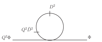
Figure 1: Supergraph composed by one $\langle\Phi_{1}\Phi_{2}\rangle$-propagator and one $\Phi^{2}(Q^{2}\Phi)^{2}$-vertex.

It follows from the supergraph of Fig. 1

$$\Gamma_{1}[\Phi]=S_{1}\Big{(}-\frac{\Sigma^{2}g}{4}\Big{)}\int\frac{d^{3}p}{(2\pi)^{3}}d^{4}\theta_{1}\big{[}Q_{1}^{2}\Phi(-p,\theta_{1})\big{]}\Phi(p,\theta_{1})\int\frac{d^{3}k}{(2\pi)^{3}}\bigg{[}-\frac{\bar{m}Q_{1}^{2}\bar{D}_{1}^{2}D_{1}^{2}\delta_{12}|_{1=2}}{k^{2}(k^{2}+\bar{m}m)}\bigg{]},$$ (34)

where $S_{1}$ is the symmetry factor. By using the identity $Q_{1}^{2}\bar{D}_{1}^{2}D_{1}^{2}\delta_{12}|_{1=2}=-k^{2}\bar{\theta}_{1}^{2}$, we obtain

$$\Gamma_{1}[\Phi]=-\frac{1}{4}S_{1}\Sigma^{2}g\bar{m}\int\frac{d^{3}p}{(2\pi)^{3}}d^{4}\theta\bar{\theta}^{2}\big{[}Q^{2}\Phi(-p,\theta)\big{]}\Phi(p,\theta)\int\frac{d^{3}k}{(2\pi)^{3}}\frac{1}{(k^{2}+\bar{m}m)}.$$ (35)

After solving the integrals, we get

$$\Gamma_{1}[\Phi]=-\frac{1}{16\pi}S_{1}\Sigma^{2}g\bar{m}^{\frac{3}{2}}m^{\frac{1}{2}}\int\frac{d^{3}p}{(2\pi)^{3}}d^{2}\theta\big{[}Q^{2}\Phi(-p,\theta)\big{]}\Phi(p,\theta).$$ (36)

In our next example, we consider the supergraph of Fig. 2.

Figure 2: Supergraph composed by two $\langle\Phi_{1}\Phi_{2}\rangle$-propagators, one $\Phi(Q^{2}\Phi)^{2}$-vertex, and one $\Phi^{3}$-vertex.

It follows from the supergraph of Fig. 2 that

$$\Gamma_{2}[\Phi] = S_{2}\Big{(}-\frac{\Sigma^{2}\lambda}{6}\Big{)}\Big{(}\frac{\lambda}{3}\Big{)}\int\frac{d^{3}p}{(2\pi)^{3}}d^{4}\theta_{1}d^{4}\theta_{2}\big{[}Q_{1}^{2}\Phi(-p,\theta_{1})\big{]}\Phi(p,\theta_{2})$$ (37)

$$\times \int\frac{d^{3}k}{(2\pi)^{3}}\bigg{[}-\frac{\bar{m}D^{2}_{2}\delta_{21}}{k^{2}(k^{2}+\bar{m}m)}\bigg{]}\bigg{[}-\frac{\bar{m}Q_{1}^{2}\bar{D}_{1}^{2}D_{1}^{2}\bar{D}^{2}_{1}\delta_{12}}{(p+k)^{2}((p+k)^{2}+\bar{m}m)}\bigg{]},$$

where $S_{2}$ is the symmetry factor. Then using $\bar{D}_{1}^{2}D_{1}^{2}\bar{D}^{2}_{1}=-(p+k)^{2}\bar{D}^{2}_{1}$ and integrating the result by parts gives

$$\Gamma_{2}[\Phi] = \frac{1}{18}S_{2}\Sigma^{2}\lambda^{2}\bar{m}^{2}\int\frac{d^{3}p}{(2\pi)^{3}}d^{4}\theta_{2}\big{[}Q_{2}^{2}\Phi(-p,\theta_{2})\big{]}\Phi(p,\theta_{2})$$ (38)

$$\times \int\frac{d^{3}k}{(2\pi)^{3}}\bigg{[}\frac{D^{2}_{2}Q^{2}_{2}\bar{D}^{2}_{2}\delta_{21}|_{2=1}}{k^{2}(k^{2}+\bar{m}m)}\bigg{]}\frac{1}{(p+k)^{2}+\bar{m}m}.$$

From $D_{2}^{2}Q_{2}^{2}\bar{D}_{2}^{2}\delta_{21}|_{2=1}=-k^{2}\bar{\theta}_{2}^{2}$ and (38), we obtain

$$\Gamma_{2}[\Phi]=\frac{1}{18}S_{2}\Sigma^{2}\lambda^{2}\bar{m}^{2}\int\frac{d^{3}p}{(2\pi)^{3}}\frac{d^{3}k}{(2\pi)^{3}}\frac{1}{(k^{2}+\bar{m}m)[(p+k)^{2}+\bar{m}m]}\int d^{2}\theta\big{[}Q^{2}\Phi(-p,\theta)\big{]}\Phi(p,\theta).$$ (39)

Finally, integrating the result, we get

$$\Gamma_{2}[\Phi]=\frac{1}{72\pi}S_{2}\Sigma^{2}\lambda^{2}\bar{m}^{2}\int\frac{d^{3}p}{(2\pi)^{3}}\frac{1}{|p|}\arcsin{\Bigg{[}\frac{|p|}{(p^{2}+4\bar{m}m)^{\frac{1}{2}}}\Bigg{]}}\int d^{2}\theta\big{[}Q^{2}\Phi(-p,\theta)\big{]}\Phi(p,\theta).$$ (40)

We notice that the one-loop quantum corrections for the effective action (36) and (40) are UV-finite. This is a natural consequence of the low dimensionality of the spacetime, namely d=3. Moreover, we also notice that the corrections (36) and (40) are holomorphic. This result is consistent with the non-renormalization theorem for deformed theories Quiral ; Quiral1 .

Now, let us study the low-energy effective action (LEEA). The LEEA is defined as the zero-order term in the covariant derivative expansion of the effective action of background superfields. Here, our goal is to calculate the one-loop correction to the LEEA within the model (30). In order to evaluate it we have to expand (30) around a background superfield $\Phi\rightarrow\Phi+\phi$ and $\bar{\Phi}\rightarrow\bar{\Phi}+\bar{\phi}$, and to keep the quadratic terms in quantum fluctuations $\phi$ and $\bar{\phi}$. Therefore, one can show that the one-loop contribution to $\Gamma[\Phi,\bar{\Phi}]$ is given by BuKu ; Grisaru :

$$\Gamma^{(1)}=-\frac{1}{2}\textrm{Tr}\ln\hat{\mathcal{H}}=-\frac{1}{2}\int d^{7}z\textrm{tr}\ln\hat{\mathcal{H}}\delta^{7}(z-z^{\prime})|_{z=z^{\prime}}.$$ (41)

where tr is the matrix trace and $\hat{\mathcal{H}}$ is an operator that is obtained from the quadratic terms in quantum fluctuations in the classical action $S[\Phi+\phi,\bar{\Phi}+\bar{\phi}]$ that we will call of $S_{2}[\Phi,\bar{\Phi};\phi,\bar{\phi}]$. Therefore, by using this prescription, we obtain from (30), after an integration by parts,

$$S_{2}[\bar{\Phi},\Phi;\bar{\phi},\phi] = \int d^{7}z\bar{\phi}\phi-\frac{1}{2}\int d^{5}\bar{z}\bar{\phi}(\bar{m}+2\bar{\lambda}\bar{\Phi}+3\bar{g}\bar{\Phi}^{2})\bar{\phi}-\frac{1}{2}\int d^{5}z\phi\Big{\{}m+2\lambda\Phi+3g\Phi^{2}$$ (42)

$$-\frac{\Sigma^{2}g}{2}(Q^{2}\Phi)^{2}-\Sigma^{2}\big{[}\lambda(Q^{2}\Phi)+\frac{g}{2}(Q^{\alpha}\Phi)(Q_{\alpha}\Phi)+3g\Phi(Q^{2}\Phi)\big{]}Q^{2}\Big{\}}\phi.$$

It is convenient to write the antichiral and chiral superfields in terms of unconstrained superfields, namely $\Phi=\bar{D}^{2}\Psi$, $\bar{\Phi}=D^{2}\bar{\Psi}$, and $\phi=\bar{D}^{2}\psi$, $\bar{\phi}=D^{2}\bar{\psi}$ Grisaru . Putting them in (42), it follows that (42) is invariant under the following Abelian gauge transformation $\delta\Psi=\bar{D}^{\dot{\alpha}}\bar{\omega}_{\dot{\alpha}}$, and $\delta\bar{\Psi}=D^{\alpha}\omega_{\alpha}$. Therefore, to fix the gauge, we add the functional Superspace

$$S_{GF}[\psi,\bar{\psi}]=\int d^{7}z\bar{\psi}(\frac{1}{2}\{\bar{D}^{2},D^{2}\}-D^{\alpha}\bar{D}^{2}D_{\alpha})\psi\ .$$ (43)

Since the theory is Abelian, the ghosts associated with this gauge fixing decouple. With all this information, we can sum up (43) and (42) to get

$$S_{2}[\Phi,\bar{\Phi};\psi,\bar{\psi}]+S_{GF}[\psi,\bar{\psi}]=\frac{1}{2}\int d^{7}z\left(\begin{array}[]{cc}\psi&\bar{\psi}\end{array}\right)\hat{\mathcal{H}}\left(\begin{array}[]{c}\psi\\ \bar{\psi}\end{array}\right)\ ,$$ (47)

where,

$$\hat{\mathcal{H}}=\left(\begin{array}[]{cc}-(\mu-\Sigma^{2}\mu_{K}-\Sigma^{2}\mu_{W}Q^{2})\bar{D}^{2}&\Box\\ \Box&-\bar{\mu}D^{2}\end{array}\right)\ ,$$ (50)

and

$$\mu=m+2\lambda\Phi+3g\Phi^{2}\ ,\ \mu_{K}=\frac{g}{2}(Q^{2}\Phi)^{2},$$ (51)

$$\mu_{W}=(\lambda+3g\Phi)(Q^{2}\Phi)+\frac{g}{2}(Q^{\alpha}\Phi)(Q_{\alpha}\Phi).$$ (52)

It is convenient to split $\hat{\mathcal{H}}$ into two parts, namely $\hat{\mathcal{H}}\equiv\hat{\mathcal{H}}_{K}+\hat{\mathcal{H}}_{W}$. Therefore, we can rewrite (41) as

$$\Gamma^{(1)}=-\frac{1}{2}\textrm{Tr}\ln(\hat{\mathcal{H}}_{K}+\hat{\mathcal{H}}_{W})=-\frac{1}{2}\textrm{Tr}\ln\hat{\mathcal{H}}_{K}-\frac{1}{2}\textrm{Tr}\ln(\hat{1}+\hat{\mathcal{H}}_{K}^{-1}\hat{\mathcal{H}}_{W})\equiv\Gamma_{K}^{(1)}+\Gamma_{W}^{(1)},$$ (53)

where

$$\hat{\mathcal{H}}_{K}=\left(\begin{array}[]{cc}-(\mu-\Sigma^{2}\mu_{K})\bar{D}^{2}&\Box\\ \Box&-\bar{\mu}D^{2}\end{array}\right)\ ,\ \hat{\mathcal{H}}_{W}=\left(\begin{array}[]{cc}\Sigma^{2}\mu_{W}Q^{2}\bar{D}^{2}&0\\ 0&0\end{array}\right)\ ,$$ (58)

$$\hat{\mathcal{H}}^{-1}_{K}=\frac{1}{\Box}\left(\begin{array}[]{cc}\displaystyle\bar{\mu}\frac{D^{2}}{\Box-(\mu-\Sigma^{2}\mu_{K})\bar{\mu}}&\displaystyle 1+\frac{\bar{\mu}(\mu-\Sigma^{2}\mu_{K})D^{2}\bar{D}^{2}}{\Box\big{[}\Box-\bar{\mu}(\mu-\Sigma^{2}\mu_{K})\big{]}}\\ \displaystyle 1+\frac{(\mu-\Sigma^{2}\mu_{K})\bar{\mu}\bar{D}^{2}D^{2}}{\Box\big{[}\Box-(\mu-\Sigma^{2}\mu_{K})\bar{\mu}\big{]}}&\displaystyle(\mu-\Sigma^{2}\mu_{K})\frac{\bar{D}^{2}}{\Box-\bar{\mu}(\mu-\Sigma^{2}\mu_{K})}\end{array}\right)\ .$$ (61)

The first term in (53) can be calculated following the same steps as in Grisaru , then we can simply repeat all this procedure. Therefore, after the calculation of the matrix and functional trace, we get

$$\Gamma_{K}^{(1)}=-\frac{1}{2}\textrm{Tr}\ln\hat{\mathcal{H}}_{K}=\frac{1}{2}\int d^{7}z\int\frac{d^{3}k}{(2\pi)^{3}}\frac{1}{k^{2}}\ln\Big{[}1+\frac{\bar{\mu}(\mu-\Sigma^{2}\mu_{K})}{k^{2}}\Big{]}\ .$$ (62)

By integrating and substituting the expressions (51), we get

$$\Gamma_{K}^{(1)}=\frac{1}{4\pi}\int d^{7}z\Big{[}\big{(}\bar{m}+2\bar{\lambda}\bar{\Phi}+3\bar{g}\bar{\Phi}^{2}\big{)}\big{(}m+2\lambda\Phi+3g\Phi^{2}-\frac{1}{2}\Sigma^{2}g(Q^{2}\Phi)^{2}\big{)}\Big{]}^{\frac{1}{2}}.$$ (63)

This result corresponds to the one-loop Kähler effective potential, it is UV-finite, and we notice that the functional structure of (63) does not involve any logarithmlike dependence, which is usually found in four-dimensional theories. One can point out that the one-loop finiteness is a characteristic feature of the three-dimensional (in particular, supersymmetric) theories, see f.e. ourEP . Besides, in the limit $\Sigma\rightarrow 0$, we recover the one-loop Kähler effective potential for the commutative theory studied in BMS . It is worth to point out that if we had ”turned off” the quartic interaction ($g=0$), we would have got the undeformed result in (63). In other words, we would have got the one-loop Kähler effective potential with unbroken ${\mathcal{N}}=2$ supersymmetry.

Let us move on and calculate the second term in (53), then we have

$$\Gamma_{W}^{(1)} = -\frac{1}{2}\textrm{Tr}\ln(\hat{1}+\hat{\mathcal{H}}_{K}^{-1}\hat{\mathcal{H}}_{W})$$ (68)

$$= -\frac{1}{2}\textrm{Tr}\ln\Bigg{[}\left(\begin{array}[]{cc}1&0\\ 0&1\end{array}\right)+\left(\begin{array}[]{cc}\displaystyle\frac{\Sigma^{2}\bar{\mu}\mu_{W}}{\Box-(\mu-\Sigma^{2}\mu_{K})\bar{\mu}}Q^{2}\frac{D^{2}\bar{D}^{2}}{\Box}&0\\ \displaystyle\frac{\Sigma^{2}\mu_{W}}{\Box-(\mu-\Sigma^{2}\mu_{K})\bar{\mu}}Q^{2}\bar{D}^{2}&0\end{array}\right)\Bigg{]}.$$

By calculating the matrix trace and writing the integral over whole superspace as $\int d^{7}z=\int d^{5}z\bar{D}^{2}$, we get

$$\Gamma_{W}^{(1)} = -\frac{1}{2}\textrm{Tr}\Bigg{[}\ln\bigg{(}1+\frac{\Sigma^{2}\bar{\mu}\mu_{W}}{\Box-(\mu-\Sigma^{2}\mu_{K})\bar{\mu}}Q^{2}\bigg{)}\frac{D^{2}\bar{D}^{2}}{\Box}\Bigg{]}$$ (69)

$$= -\frac{1}{2}\int d^{5}z\int\frac{d^{3}k}{(2\pi)^{3}}\ln\bigg{(}1-\frac{\Sigma^{2}\bar{\mu}\mu_{W}}{k^{2}+(\mu-\Sigma^{2}\mu_{K})\bar{\mu}}Q^{2}\bigg{)}\bar{D}^{2}\delta^{4}(\theta-\theta^{\prime})|_{\theta=\theta^{\prime}}.$$

This is the exact result. However, the integral in (69) is very complicated due to the fact that we are considering $Q_{\alpha}\Phi\neq 0$. In order to perform the integral above, we will consider the approximation in which $\Sigma$ is very small. This approximation is reasonable, since we are calculating the LEEA and at low-energies is expected that $\Sigma$ be small. Therefore, we can rewrite (69) as

$$\Gamma_{W}^{(1)} = \frac{1}{2}\Sigma^{2}\int d^{5}z\int\frac{d^{3}k}{(2\pi)^{3}}\frac{\bar{\mu}\mu_{W}}{k^{2}+\bar{\mu}\mu}Q^{2}\bar{D}^{2}\delta^{4}(\theta-\theta^{\prime})|_{\theta=\theta^{\prime}}+{\mathcal{O}}(\Sigma^{4})$$ (70)

$$= -\frac{1}{8\pi}\Sigma^{2}\bar{\mu}^{\frac{3}{2}}\int d^{5}z\mu^{\frac{1}{2}}\mu_{W}+{\mathcal{O}}(\Sigma^{4}).$$

Finally, turning off the antichiral superfield ($\bar{\Phi}=0\Rightarrow\bar{\mu}=\bar{m}$), we obtain

$$\Gamma_{W}^{(1)}=-\frac{1}{8\pi}\Sigma^{2}\bar{m}^{\frac{3}{2}}\int d^{5}z\big{(}m+2\lambda\Phi+3g\Phi^{2}\big{)}^{\frac{1}{2}}\big{[}(\lambda+3g\Phi)(Q^{2}\Phi)+\frac{g}{2}(Q^{\alpha}\Phi)(Q_{\alpha}\Phi)\big{]}+{\mathcal{O}}(\Sigma^{4}).$$ (71)

This result corresponds to the one-loop chiral effective potential. We notice that in the limit $\Sigma\rightarrow 0$, we get from (69) and (71), $\Gamma_{W}^{(1)}=0$, which is consistent with the vanishing of the one-loop chiral effective potential for the commutative theory, as argued in BMS . From the result (69), we can infer that the higher-order terms in (71) are UV-finite. The argument is similar to that used in TO and goes as follows: if we expand the logarithm in (69), only one of the factors $Q^{2}$ will act on $\bar{D}^{2}\delta^{4}(\theta-\theta^{\prime})|_{\theta=\theta^{\prime}}$ due to the fact that $Q^{3}=0$, so that $Q^{2}\bar{D}^{2}\delta^{4}(\theta-\theta^{\prime})|_{\theta=\theta^{\prime}}=1$. The other factors will act on $G(k^{2})=\frac{1}{k^{2}+(\mu-\Sigma^{2}\mu_{K})\bar{\mu}}$, so that every time that $Q^{2}$ acts on $G(k^{2})$ the UV convergence will not be worsened, on the contrary, $Q_{\alpha}G(k^{2})\sim\frac{1}{k^{4}}$. Since (70) is UV-finite and every time that $Q^{2}$ acts on $G(k^{2})$ the UV-convergence will be improved, it follows that the higher-order terms in (71) will be UV finite.

We developed a new formulation of the three-dimensional noncommutative superspace which turns out to be more convenient for the superfield calculation than those ones described in earlier . Within this description, one can straightforwardly use all methods and approaches which have been well developed for the four-dimensional noncommutative superfield theories. In particular, just as it takes place in the four-dimensional field theories, one should introduce a partial breaking of the ${\cal N}=2$ supersymmetry to implement the fermionic noncommutativity. We have constructed the chiral superfield model within this approach and explicitly calculated the two-point function and the one-loop low-energy effective action for this theory.

It is interesting to note that in this theory, from a formal viewpoint one meets the Lorentz symmetry breaking introduced through a constant matrix $\Sigma^{\alpha\beta}$ which is equivalent to a constant vector $\Sigma^{m}=\frac{1}{\sqrt{2}}(\gamma^{m})_{\alpha\beta}\Sigma^{\alpha\beta}$. However, within this paper, all quantum corrections we found depend on the noncommutativity matrix only implicitly, through a scalar factor $\Sigma^{2}=\Sigma_{\alpha\beta}\Sigma^{\alpha\beta}$. This resembles the fact that within other Lorentz-breaking extension of the superfield approach, that is, the so-called aether superspace aether ; aether1 , the Lorentz-breaking parameters enter the final result also through a scalar factor representing itself as a determinant of some matrix depending on the Lorentz-breaking parameter. This situation is typical for the contributions to the effective potential which do not involve derivatives of background superfields, as well as for some other low-order contributions which were considered in our paper. Nevertheless, in principle the contributions in which the noncommutativity matrix itself, and not only the scalars constructed on its base, enters, are possible, for example, the terms like $\Sigma^{\alpha\beta}D_{\alpha}\Phi\bar{D}_{\beta}\bar{\Phi}$, so, in general, the terms depending on the Lorentz-breaking parameter in an explicit form are not excluded.

The natural continuation of this study would consist in introducing the supergauge symmetry and models for supergauge field, and in studying of higher loop corrections, within this methodology. We are planning to do this in a forthcoming paper.

Acknowledgements. This work was partially supported by Conselho Nacional de Desenvolvimento Científico e Tecnológico (CNPq). The work by A. Yu. P. has been supported by the CNPq project No. 303783/2015-0.

References

• (1) S. J. Gates, Jr., M. T. Grisaru, M. Rocek and W. Siegel, Superspace or One Thousand and One Lessons in Supersymmetry, Benjamin/Cummings, 1983; Front. Phys. 58 (1983) 1-548, hep-th/0108200.
• (2) S. Ferrara, M. A. Lledo, JHEP 0005, 008 (2000), hep-th/0002084.
• (3) D. Klemm, S. Penati, L. Tamassia, Class. Quant. Grav. 20, 2905 (2003), hep-th/0104190.
• (4) N. Seiberg, JHEP 0306, 010 (2003), hep-th/0305248.
• (5) M. S. Berger, V. A. Kostelecky, Phys. Rev. D65, 091701 (2002), hep-th/0112243.
• (6) N. Berkovits, N. Seiberg, JHEP 0307, 010 (2003), hep-th/0306226.
• (7) R. Britto, B. Feng, Phys. Rev. Lett. 91, 201601 (2003), hep-th/0307165.
• (8) A. Romagnoni, JHEP 0310, 016 (2003), hep-th/0307209.
• (9) M. T. Grisaru, S. Penati, A. Romagnoni, JHEP 08, 003 (2003), hep-th/0307099.
• (10) S. Penati, A. Romagnoni, JHEP 0502, 064 (2005), hep-th/0412041.
• (11) M. T. Grisaru, S. Penati, A. Romagnoni, JHEP 0602, 043 (2006), hep-th/0510175.
• (12) T. Araki, K. Ito, A. Ohtsuka, Phys. Lett. B573, 209 (2003), hep-th/0307076.
• (13) O. Lunin, S.-J. Rey, JHEP 0309, 045 (2003), hep-th/0307275.
• (14) I. Jack, D. R. T. Jones, L. A. Worthy, Phys. Lett. B611, 199 (2005), hep-th/0412009.
• (15) I. Jack, D. R. T. Jones, L. A. Worthy, Phys. Rev. D72, 065002 (2005), hep-th/0505248.
• (16) S. Ferrara, E. A. Ivanov, O. Lechtenfeld, E. Sokatchev, B. Zupnik, Nucl. Phys. B704, 154 (2005), hep-th/0405049.
• (17) E. A. Ivanov, B. M. Zupnik, Theor. Math. Phys. 142, 197 (2005), hep-th/0405185.
• (18) A. T. Banin, I. L. Buchbinder, N. G. Pletnev, JHEP 0407, 011 (2004), hep-th/0405063.
• (19) O. D. Azorkina, A. T. Banin, I. L. Buchbinder, N. G. Pletnev, Mod. Phys. Lett. A20, 1423 (2005), hep-th/0502008.
• (20) O. D. Azorkina, A. T. Banin, I. L. Buchbinder, N. G. Pletnev, Phys. Lett. B633, 389 (2006), hep-th/0509193;
• (21) O. D. Azorkina, A. T. Banin, I. L. Buchbinder, N. G. Pletnev, Phys. Lett. B635, 50 (2006), hep-th/0601045.
• (22) A. F. Ferrari, M. Gomes, J. R. Nascimento, A. Yu. Petrov, A. J. da Silva, Phys.Rev. D74 (2006) 125016, hep-th/0607087.
• (23) M. Faizal, Phys. Rev. D84, 106011 (2011), arXiv: 1102.2013.
• (24) M. Faizal, Europhys. Lett. 98, 31003 (2012), arXiv: 1204.1191.
• (25) M. Faizal, D. J. Smith, Phys. Rev. D87, 025019 (2013), arXiv: 1211.3654.
• (26) N. J. Hitchin, A. Karlhede, U. LindstrΓΆm, and M. Rocek, Commun. Math. Phys. 108, 535 (1987).
• (27) I. L. Buchbinder, N. G. Pletnev, I. B. Samsonov, JHEP 1004, 124 (2010), arXiv: 1003.4806.
• (28) I. L. Buchbinder, N. G. Pletnev, I. B. Samsonov, JHEP 1101, 121 (2011), arXiv: 1010.4967.
• (29) I. L. Buchbinder, B. S. Merzlikin, I. B. Samsonov, Nucl. Phys. B860, 87 (2012) arXiv: 1201.5579.
• (30) F. S. Gama, M. Gomes, J. R. Nascimento, A. Yu. Petrov, A. J. da Silva, Phys.Rev. D89, 085018 (2014), arXiv: 1401.6839.
• (31) I. L. Buchbinder, N. G. Pletnev, I. B. Samsonov, JHEP 04, 124 (2010), arXiv: 1003.4806.
• (32) R. Britto, B. Feng and S.-J. Rey, JHEP 07, 067 (2003), hep-th/0306215.
• (33) S. Terashima and J.-T. Yee, JHEP 12, 053 (2003), hep-th/0306237.
• (34) I. L. Buchbinder and S. M. Kuzenko, Ideas and Methods of Supersymmetry and Supergravity, IOP Publishing, Bristol and Philadelphia, 1995.
• (35) M. T. Grisaru, M. Rocek, and R. von Unge, Phys. Lett. B383, (1996) 415, hep-th/9605149.
• (36) T. Ohsaku, JHEP 02, 021 (2008), hep-th/0603135.
• (37) A. F. Ferrari, M. Gomes, A. C. Lehum, J. R. Nascimento, A. Yu. Petrov, A. J. da Silva, Phys. Lett. B678, 500 (2009), arXiv: 0901.0679.
• (38) C. F. Farias, A. C. Lehum, J. R. Nascimento, A. Yu. Petrov, Phys. Rev. D86, 065035 (2012), arXiv: 1206.4508.
• (39) A. C. Lehum, J. R. Nascimento, A. Yu. Petrov, A. J. da Silva, Phys. Rev. D88, 045022 (2013), arXiv: 1305.1812.