On Instability of Squashed Spheres in the Kaluza-Klein Theory

Abstract

We study in Kaluza-Klein theories stability of the extra space against “squashing”, in other words, the homogeneous deformation. Quantum fluctuations of matter fields at one-loop level are taken into consideration. We calculate the effective potential in models of the type, $M^{4}\times S^{3}$ and $M^{4}\times S^{7}$. It is found that in the case of scalar matter fields the stability depends on the coupling to the scalar curvature.

1 Introduction

Many problems on the unification of interactions in higher dimensions have been discussed recently.[1] In Kaluza-Klein theories the ground state is taken to be a product of four dimensional space-time and some compact homogeneous space whose isometry corresponds to the gauge symmetry. The length scale associated with the “extra” dimensions must be comparable to the Planck length ($\sim 10^{-33}$cm) in order for gauge couplings in the theory to be of order of unity.[2] The energy scale of excited modes on the internal space is therefore the Planck energy ($\sim 10^{19}$ GeV). One of the difficulties in this approach is how one can find a static compactified solution of the Einstein equation which has the desired size of the extra space. Many authors obtained static solutions in models which include classical bosonic fields and/or fermion condensations. On the other hand, Candelas and Weinberg [3] considered quantum effects of matter fields and showed that there are solutions in which the background geometry is $M^{4}\times S^{N}$. They showed that the number of matter fields would determine the magnitude of the gauge coupling constant and the stability against uniform dilatations of the scale of $S^{N}$. A special case of the more general spacetime $M^{4}\times S^{M}\times S^{N}$ is considered by Kikkawa et al.[4] Their stable solutions due to quantum effects of matter fields give the ratio of coupling constants. Their model is a proto-type of the so-called “standard model” of interactions (i.e., a model of the product gauge group). Recently Lim [5] and Okada [6] discussed the symmetry breaking in the Kaluza-Klein theories. They found that symmetries of the isometry group are broken through quantum effects of (minimally or conformally coupled) scalar matter fields. This symmetry breaking corresponds to a deformation of the extra space. lt may be said that their models correspond to grand unified theories which include spontaneous symmetry breakings.

In this paper, we investigate the stability of extra space against homogeneous deformation in two cases. In one case, the extra space is either $S^{3}$ or $S^{7}$ with non-minimally coupled scalar fields, and in the other case the extra space is $S^{3}$ with Dirac fermion fields.

The present paper is organized as follows. In §2, 1Fe consider the metric $M^{4}\times(\mbox{squashed~{}}S^{3})$ and relation of the gauge symmetry breaking and the deformation of spheres. In §3, we calculate the one-loop quantum effective potential for the metric of $M^{4}\times S^{3}$ and discuss the stability against “squashing”. The stability for the background geometry of $M^{4}\times S^{7}$ is also discussed in §4. The last section is devoted to discussion.

2 Homogeneous deformations of $S^{3}$

The symmetry of $S^{3}$ is well known in particular through the investigation of the mixmaster universe model. We can express a line element of three dimensional space as follows:

$$d\ell^{2}=a^{2}\sigma_{1}^{2}+b^{2}\sigma_{2}^{2}+c^{2}\sigma_{3}^{2}$$ (1)

and

$$\sigma_{1} = -\sin\psi d\theta+\cos\psi\sin\theta d\phi\,,$$

$$\sigma_{2} = \cos\psi d\theta+\sin\psi\sin\theta d\phi\,,$$

$$\sigma_{3} = d\psi+\cos\theta d\phi\,.$$

Here $a$, $b$ and $c$ are scale factors, and in the case $a=b=c$, this line element corresponds to that of a maximally symmetric 3-sphere.

When three scale factors take different values, this space has lower symmetry. We will denote this deformable space as $\hat{S}^{3}$ or “squashed” $S^{3}$.

If one uses this space as the extra space in the Kaluza-Klein theory, the gauge symetry breaking can be discussed. To see this, we consider the seven dimensional geometry as (Kaluza-Klein ansatz):

$$ds^{2}=\eta_{\mu\nu}dx^{\mu}dx^{\nu}+a^{2}s_{1}^{2}+b^{2}s_{2}^{2}+c^{2}s_{3}^{2}$$ (2)

and $s_{i}=\sigma_{i}+K_{i}^{\alpha}A_{\mu}^{\alpha}(x)dx^{\mu}$, ($i=1,2,3;\alpha=1,2,\dots,6$) where $\eta_{\mu\nu}={\rm diag}(-1,1,1,1)$, $x^{\mu}$ are coordinates of four dimensional flat space, and $K_{i}^{\alpha}$ are $i$-th components of six Killing vectors on $S^{3}$. The isometry group of $S^{3}$ is $SO(4)$, which has six generators.

In this case, the four dimensional effective action of gauge fields after being reduced from the seven dimensional Einstein-Hilbert action is given by [7]

$$\int d^{4}x\left[-\frac{1}{4}\left\{a^{2}(F^{1}_{\mu\nu})^{2}+b^{2}(F^{2}_{\mu\nu})^{2}+c^{2}(F^{3}_{\mu\nu})^{2}\right.\right.$$

$$\quad\left.\left.+\frac{1}{3}(a^{2}+b^{2}+c^{2})\{(F^{4}_{\mu\nu})^{2}+(F^{5}_{\mu\nu})^{2}+(F^{6}_{\mu\nu})^{2}\}\right\}\right.$$

$$\quad-\left.\frac{1}{2}\left\{\frac{(b^{2}-c^{2})^{2}}{b^{2}c^{2}}(A^{1}_{\mu})^{2}+\frac{(c^{2}-a^{2})^{2}}{c^{2}a^{2}}(A^{2}_{\mu})^{2}+\frac{(a^{2}-b^{2})^{2}}{a^{2}b^{2}}(A^{3}_{\mu})^{2}\right\}\right]\,.$$ (3)

There appear mass terms of gauge bosons in general. From (3) gauge symmetries are shown to be

$$SU(2)\times SU(2)\sim SO(4) \mbox{when~{}}a=b=c\,,$$

$$SU(2)\times U(1) \mbox{when~{}}a=b\neq c\quad\mbox{etc}\,,$$

$$SU(2) \mbox{when~{}}a\neq b\neq c\,.$$

The gauge symmetry breaking of this type is extensively investigated by Okada.[6] He found that the quantum effect of conformally coupled scalar field would break the symmetry,

We shall consider here only the possibility of breaking of maximal symmetry, that is, the stability of “round” sphere, for simplicity. However, we deal with quantum effects of non-minimally coupled scalar fields generally, as well as fermion matter fields.

3 Stability of $\hat{S}^{3}$

In order to calculate one-loop quantum effects, we must know the spectrum of the wave operator on $\hat{S}^{3}$.

First, let us consider the scalar field coupled to gravity nonminimally as the matter field. The Lagrangian density (for matter+gravity) is

$$L=-\frac{1}{2}(\partial_{M}\Phi)^{2}+\frac{1}{2}\xi R\Phi^{2}-\frac{1}{16\pi\bar{G}}(R+2\lambda)\,,$$ (4)

where $R$ is the scalar curvature.

The scalar boson mass matrix on $\hat{S}^{3}$ can be written as

$$M^{2}=\frac{1}{a^{2}}L_{1}^{2}+\frac{1}{b^{2}}L_{2}^{2}+\frac{1}{c^{2}}L_{3}^{2}-\xi\tilde{R}\,,$$ (5)

where

$$\tilde{R}=-\frac{1}{2a^{2}b^{2}c^{2}}(2b^{2}c^{2}+2c^{2}a^{2}+2a^{2}b^{2}-a^{4}-b^{4}-c^{4})\,.$$ (6)

Operators $L_{1},L_{2}$ and $L_{3}$ satisfy the same algebraic relation as the angular momentum.[8] When $a=b$, the mass matrix can be diagonalized as

$$M^{2}_{(L,m)}=\frac{1}{a^{2}}\{L(L+1)-m^{2}\}+\frac{1}{c^{2}}m^{2}-\xi\tilde{R}$$ (7)

with $L=0,1/2,1,\dots,m=-L,-L+1,\dots,L$.

We use the dimensional regularization to calculate the effective potential $V_{1}$ as in Ref. [3]:

$$V_{1}=-\frac{1}{2(4\pi)^{2}}\Gamma\left(-\frac{n}{2}\right){\rm Tr~{}}D\,(M^{2})^{n/2}\,,\qquad n\rightarrow 4\,,$$ (8)

where $D$ is the degeneracy of the states. In our case, $D=2L+1$. The one-loop effective potential for $M^{4}\times\hat{S}^{3}$ is then given by

$$V_{1}=-\frac{1}{2(4\pi)^{2}}\frac{1}{(2a)^{4}}\Gamma\left(-\frac{n}{2}\right)\sum_{l=1}^{\infty}\,l\,\sum_{m}\left[l^{2}-1+4m^{2}\left(\frac{a^{2}}{c^{2}}-1\right)-\xi\tilde{R}\cdot(2a)^{2}\right]^{n/2}\,,$$ (9)

when $a=b$. The summation on $m$ is taken for $m=-(l-1)/2,-(l-3)/2,\dots,(l-1)/2$.

In the general case ($a\neq b\neq c$) , let us use the following parametrization:

$$a = \bar{a}\exp\left(u+\frac{\sqrt{5}}{2}v+\frac{\sqrt{15}}{2}w\right)\,,$$

$$b = \bar{a}\exp\left(u+\frac{\sqrt{5}}{2}v-\frac{\sqrt{15}}{2}w\right)\,,$$

$$c = \bar{a}\exp\left(u-{\sqrt{5}}v\right)\,.$$ (10)

$v$ or $w$ represents presence of a nonvanishing deformation from the sphere, keeping the volume of extra space constant. Following Moss,[9] we choose coordinates in which the metric takes the form

$$ds^{2}=e^{-3u}\eta_{\mu\nu}dx^{\prime}{}^{\mu}dx^{\prime}{}^{\nu}+dl^{2}\,.$$ (11)

The effective potential (including the tree level potential) can be written as

$$U = \frac{2}{15}e^{-3u}\left[\lambda-\frac{1}{(2\bar{a})^{2}}e^{-2u}\{4e^{-\sqrt{5}v}\cosh\sqrt{15}w\right.$$ (12)

$$\left.-e^{-4\sqrt{5}v}-4e^{2\sqrt{5}v}(\sinh\sqrt{15}w)^{2}\}+8\pi\bar{G}\frac{J(v,w)}{2\pi^{2}(2\bar{a})^{7}}e^{-7u}\right]\,.$$

The first term includes the cosmological constant $\lambda$ and the second term comes from the curvature of the extra space. The last term includes quantum effects, while $J(v,w)$ is defined as

$$V_{1}=\frac{e^{-4u}}{(2\bar{a})^{4}}J(v,w)\,.$$ (13)

Then Einstein equations give

$$\frac{1}{2}\{(\partial_{\mu}u)^{2}+(\partial_{\mu}v)^{2}+(\partial_{\mu}w)^{2}\}+U = 0\,,$$

$$-\partial^{\mu}\partial_{\mu}u+\frac{\partial U}{\partial u} = 0\,,$$

$$-\partial^{\mu}\partial_{\mu}v+\frac{\partial U}{\partial v} = 0\,,$$

$$-\partial^{\mu}\partial_{\mu}w+\frac{\partial U}{\partial w} = 0\,.$$ (14)

Therefore, in order to obtain the static stable solution without deformation from the spherical symmetry ($v=w=0$), we can choose $\lambda$ and $\bar{a}$ such that $U(u=v=w=0)=\partial U/\partial u(u=v=w=0))=0$ and $\partial^{2}U/\partial u^{2}(u=v=w=0)>0$ provided that $J(v=w=0)\equiv J_{0}>0$. Our choice is

$$\lambda=\frac{8\pi\bar{G}}{2\pi^{2}(2\bar{a})^{7}}\frac{5}{2}J_{0}\,,\quad\frac{6}{(2\bar{a})^{2}}=\frac{8\pi\bar{G}}{2\pi^{2}(2\bar{a})^{7}}\cdot 7J_{0}\,.$$ (15)

Here, we consider the stability against the defomations. It is easily found that $\partial U/\partial v=\partial U/\partial w=0$ and $\partial^{2}U/\partial v^{2}=\partial^{2}U/\partial w^{2}$ at $u=v=w=0$ hold in our model (see Appendix A). The stability condition against the perturbation of $v$ is then

$$\frac{\partial^{2}U}{\partial v^{2}}(u=v=w=0)=\frac{2}{15}\frac{8\pi\bar{G}}{2\pi^{2}(2\bar{a})^{7}}\delta>0\,,$$ (16)

where

$$\delta\equiv 70J_{0}+\frac{\partial^{2}J}{\partial v^{2}}(v=w=0)\,.$$

The numerical calculation of the effective potential is performed by the method shown in Appendix A. Figure 1 shows $J(v)$; $J(v,w=0)$ plotted against $v$. We show $\delta$ and $J_{0}$ against the scalar-curvature coupling $\xi$ in Fig. 2. It is found that the maximally symmetric $\hat{S}^{3}$ can be stabilized when $0.007\leq\xi\leq 0.198$.

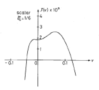
Figure 1: The result of the numerical calculations for $J(v)$ due to a scalar field ($\xi=1/6$) in the case $M^{4}\times\hat{S}^{3}$.

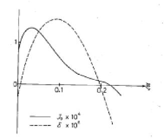
Figure 2: $J_{0}$ and $\delta$ are plotted against $\xi$ in the case $M^{4}\times\hat{S}^{3}.$

We also calculate the quantum effect of Dirac fermion field (see Appendix A). $J(v)$ is shown in Fig. 3. We find

$$\delta\approx-0.176<0.$$

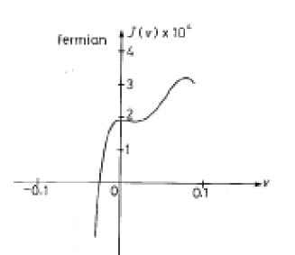
Figure 3: The result of the numerical calculations for $J(v)$ due to a fermion field in the case $M^{4}\times\hat{S}^{3}$.

From (16), it is impossible to stabilize $S^{3}$ with the quantum effect of Dirac fermion fields only.

4 The case $M^{4}\times\hat{S}^{7}$

It is well known that $S^{7}$ is deformed homogeneously, or “squashed”.[10] The deformable $S^{7}$ has the following line element:

$$dl^{2}=a^{2}\left(d\mu^{2}+\frac{1}{4}\sin^{2}\mu\sum_{i=1}^{3}\omega_{i}^{2}\right)+\frac{1}{4}\sum_{i=1}^{3}b_{i}^{2}\left(\nu_{i}+\cos\mu\omega_{i}\right)^{2}\,,$$ (17)

where

$$\nu_{i}=\sigma_{i}+\Sigma_{i}\,,\quad\omega_{i}=\sigma_{i}-\Sigma_{i}$$

and they satisfy the algebra, such as

$$d\sigma_{1}=-\sigma_{2}\wedge\sigma_{3}\,,\quad d\Sigma_{1}=-\Sigma_{2}\wedge\Sigma_{3}\,.$$

The scalar curvature is

$$-\left[\frac{12}{a^{2}}-\frac{b_{1}^{2}+b_{2}^{2}+b_{3}^{2}}{a^{4}}+\frac{1}{2b_{1}^{2}b_{2}^{2}b_{3}^{2}}(2b_{2}^{2}b_{3}^{2}+2b_{3}^{2}b_{1}^{2}+2b_{1}^{2}b_{2}^{2}-b_{1}^{4}-b_{2}^{4}-b_{3}^{4})\right]\,.$$ (18)

For simplicity, we take $b_{1}=b_{2}=b_{3}=b$.

Similarly to the last section, let us parametrize $a$ and $b$ as

$$a = \bar{a}\exp\left(u+\frac{3}{2}\sqrt{\frac{3}{2}}v\right)\,,$$

$$b = \bar{a}\exp\left(u-2\sqrt{\frac{3}{2}}v\right)\,.$$ (19)

The mass spectrum on $\hat{S}^{7}$ was already given by Nilsson and Pope.[11] We calculate the quantum effect of nonminimally coupled scalar fields in the similar way as in the last section (see Appendix B). The result is shown in shown in Fig. 4. Here $\beta$ indicates the effective four dimensional Newton constant (see Appendix B), as given by Ref. [3]. Then we consider that the region of $\xi$ in which $\beta$ is negative has no physical meaning.

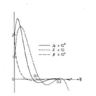
Figure 4: $J_{0}$, $\delta$ and $\beta$ are plotted against $\xi$ in the case $M^{4}\times\hat{S}^{7}$.

We find that in order to stabilize $S^{7}$, $\xi$ must fall in a region given by $0<\xi\leq 0.054$ or $0.193\leq\xi\leq 0.218$.

5 Discussion

In the present paper, we have investigated the stability of deformable spheres. It is shown that the stability depends on the coupling $\xi$ to the scalar curvature in the case that the quantum effect of scalar fields is taken into account.

We have studied very limited types of deformations. The structures of the deformable spheres have mathematically interesting features. It is also interesting that $M^{4}\times\mbox{(extra space)}$ is regarded as the result of some sorts of deformations, since we study a spontaneous compactification of a dimensional reduction as an effect of dynamical time evolution of scale factors in the cosmological context. In addition, deformations of extra spaces may require some modification in the scenario of the “Kaluza-Klein Inflation [12]”.

Appendix A

We give the details of calculations of the effective potential for the model, the geometry of which is $M^{4}\times\hat{S}^{3}$.

Scalar fields

We rewrite $J$ as

$$J(v,w)=-\frac{e^{-2\sqrt{5}v}}{2(4\pi)^{2}}\Gamma\left(-\frac{n}{2}\right)\sum_{l=1}^{\infty}\,l{\rm tr~{}}[M_{0}^{2}+m_{1}^{2}]^{n/2}\,,\quad n\rightarrow 4\,,$$ (20)

where

$$M_{0}^{2} = \cosh\sqrt{15}w\,(l^{2}-1)+2\xi\{4\cosh\sqrt{15}w-e^{-3\sqrt{5}v}-4e^{-3\sqrt{5}v}(\sinh\sqrt{15}w)^{2}\}\,,$$

$$m_{1}^{2} = 4(e^{3\sqrt{5}v}-\cosh\sqrt{15}w)L_{3}^{2}-2\sinh\sqrt{15}w(L_{+}^{2}+L_{-}^{2})$$

and

$$L_{+}=L_{1}+iL_{2}\,,\quad L_{-}=L_{1}-iL_{2}\,.$$

Therefore,

$$J_{0}=J(0,0)=-\frac{1}{2(4\pi)^{2}}\Gamma\left(-\frac{n}{2}\right)\sum_{l=1}^{\infty}l^{2}(l^{2}-1+6\xi)^{n/2}\,,\quad n\rightarrow 4\,.$$

This agrees with $C_{3}^{(0)}$ ($C_{3}^{conformal}$) in Ref. [3] when $\xi=0$ ($\xi=5/24$).

The expressions for $\partial J/\partial v,\partial J/\partial w,\partial^{2}J/\partial v^{2},\partial^{2}J/\partial w^{2}$ and $\partial^{2}J/\partial v\partial w$ is derived from the perturbative method. They are found to be

$$\frac{\partial J}{\partial v}(v=w=0) = \frac{\partial J}{\partial w}(v=w=0)=0\,,$$

$$\frac{\partial^{2}J}{\partial v^{2}}(v=w=0) = \frac{\partial^{2}J}{\partial v^{2}}(v=w=0)$$

$$= 20J_{0}-\frac{4}{(4\pi)^{2}}\Gamma\left(-\frac{n}{2}\right)\sum_{l}l^{2}(l^{2}-1)(l^{2}-4)(l^{2}-1+6\xi)^{n/2-2}$$

$$+\frac{180}{(4\pi)^{2}}\Gamma\left(-\frac{n}{2}\right)\sum_{l}l^{2}(l^{2}-1+6\xi)^{n/2-1}\,,$$

$$\frac{\partial^{2}J}{\partial v\partial w}(v=w=0) = 0\,.$$ (21)

In order to evaluate these quantities, we use the following identity:

$$\Gamma\left(-\frac{n}{2}\right)(M^{2})^{n/2}=\int_{0}^{\infty}dt\,t^{-n/2-1}\exp(-tM^{2})\,.$$ (22)

For example, it leads to

$$J_{0}=-\frac{1}{32\pi^{2}}\sum_{l=1}^{\infty}l^{2}\int dt\,t^{-n/2-1}\exp\{-t(l^{2}-1+6\xi)\}\,.$$ (23)

Further, using the reaection formula [13]

$$\sum_{l=1}^{\infty}l^{2}\exp(-l^{2}t)=\frac{\sqrt{\pi}}{t^{3/2}}\left[\sum_{l=1}^{\infty}\left(\frac{1}{2}-\frac{\pi^{2}l^{2}}{t}\right)\exp\left(-\frac{\pi^{2}l^{2}}{t}\right)+\frac{1}{4}\right]\,,$$ (24)

it can be shown as

$$J_{0} = -\frac{\sqrt{\pi}}{32\pi^{2}}\int_{0}^{\infty}dt\,t^{-n/2-5/2}\exp\{-t(6\xi-1)\}\left\{\sum_{l=1}^{\infty}\left(\frac{1}{2}-\frac{\pi^{2}l^{2}}{t}\right)e^{-\frac{\pi^{2}l^{2}}{t}}+\frac{1}{4}\right\}$$ (25)

$$= -\frac{\sqrt{\pi}}{32\pi^{2}}\left[\sum_{l}\left\{\frac{(6\xi-1)^{1/2}}{\pi l}\right\}^{7/2}K_{7/2}(2(6\xi-1)^{1/2}\pi l)\right.$$

$$-\sum_{l}2\pi^{2}l^{2}\left\{\frac{(6\xi-1)^{1/2}}{\pi l}\right\}^{9/2}K_{9/2}(2(6\xi-1)^{1/2}\pi l)$$

$$\left.+\frac{1}{4}\Gamma\left(-\frac{7}{2}\right)(6\xi-1)^{7/2}\right]\,.$$

In the last line of (25) , we have used the identity including the modified Bessel function $K_{\nu}(z)$:

$$K_{\nu}(z)=\frac{1}{2}\left(\frac{z}{2}\right)^{\nu}\int_{0}^{\infty}\exp\left(-t-\frac{z^{2}}{4t}\right)t^{-\nu-1}dt\,.$$ (26)

Finally, we obtain

$$J_{0}=-\frac{1}{840\pi}(6\xi-1)^{7/2}+\frac{1}{32\pi}(6\xi-1)^{2}\sum_{l=1}^{\infty}\frac{e^{-z}}{\pi^{3}l^{3}}\left(1+\frac{9}{z}+\frac{39}{z^{2}}+\frac{90}{z^{3}}+\frac{90}{z^{4}}\right)\,,$$ (27)

where $z=2(6\xi-1)^{1/2}\pi l$.

The value of $\partial^{2}J/\partial v^{2}(v=w=0)$ is obtained in a similar way. The result is

$$\partial^{2}J/\partial v^{2}(v=w=0) = \frac{1}{12\pi}(6\xi-1)^{3/2}\{(6\xi-1)^{2}-2\}$$ (28)

$$+\frac{7}{8\pi}(6\xi-1)^{2}\sum_{l=1}^{\infty}\frac{e^{-z}}{\pi^{3}l^{3}}\left(1+\frac{9}{z}+\frac{39}{z^{2}}+\frac{90}{z^{3}}+\frac{90}{z^{4}}\right)$$

$$+\frac{3}{8\pi}(19\xi+1)(6\xi-1)^{3/2}\sum_{l=1}^{\infty}\frac{e^{-z}}{\pi^{2}l^{2}}\left(1+\frac{5}{z}+\frac{12}{z^{2}}+\frac{12}{z^{3}}\right)$$

$$+\frac{9}{4\pi}\xi(2\xi+1)(6\xi-1)\sum_{l=1}^{\infty}\frac{e^{-z}}{\pi l}\left(1+\frac{2}{z}+\frac{2}{z^{2}}\right)\,.$$

To draw Fig. 1, we use the method discussed in Appendix D of Ref. [3]. At the first step, we expand as

$$\Gamma\left(-\frac{n}{2}\right)(A+B)^{n/2}=\sum_{r=0}^{\infty}\frac{\Gamma(r-n/2)}{r!}A^{n/2-r}B^{r}(-1)^{r}\,.$$ (29)

Next, we calculate the finite sum on $m$, and use the identity

$$\Gamma\left(\frac{1}{2}z\right)\zeta(z)=\pi^{z-1/2}\Gamma\left(\frac{1-z}{2}\right)\zeta(1-z)\,.$$ (30)

The behavior in the vicinity of $v=0$ agrees with the result obtained by (28).

Fermions

The mass spectrum is shown by Dowker [14] as

$$M_{\pm}=\frac{1}{2a}\left\{\frac{1}{2}\frac{c}{a}\pm\sqrt{(2L+1)^{2}+4m^{2}\left(\frac{a^{2}}{b^{2}}-1\right)}\right\}\quad\mbox{when~{}}a=b$$ (31)

with $-(L\pm 1/2)\leq m\leq L\pm 1/2$ and $L\geq 0$ for $M_{+}$ and $L>1/2$ for $M_{-}$. The degeneracy is $2L+1$.

Consequently, we find

$$J(v))=J(v,0) = \frac{4}{2(4\pi)^{2}}e^{4\sqrt{5}v}\Gamma\left(-\frac{n}{2}\right)\left[\sum_{l=1}^{\infty}l\sum_{q=0}^{l}\left\{\sqrt{l^{2}+4\gamma q(l-q)}+\frac{1}{2}e^{-3\sqrt{5}v}\right\}^{n}\right.$$

$$+\sum_{l=1}^{\infty}l\left.\sum_{q=1}^{l-1}\left\{\sqrt{l^{2}+4\gamma q(l-q)}-\frac{1}{2}e^{-3\sqrt{5}v}\right\}^{n}\right]$$

$$= \frac{1}{4\pi^{2}}e^{4\sqrt{5}v}\left[\sum_{r=0}^{\infty}\frac{\Gamma(2r-n)}{\Gamma(-r)(2r)!}\Gamma\left(-\frac{n}{2}\right)\right.$$

$$\times\sum_{l=1}^{\infty}l\sum_{q=0}^{l}[l^{2}+4\gamma q(l-q)]^{n/2-r}\left(\frac{1}{2}e^{-3\sqrt{5}v}\right)^{2r}$$

$$\left.-\sum_{r=0}^{\infty}\frac{\Gamma(2r+1-n)}{\Gamma(-n)(2r+1)!}\Gamma\left(-\frac{n}{2}\right)\zeta(2r-n)\left(\frac{1}{2}e^{-3\sqrt{5}v}\right)^{2r+1}\right]$$

with

$$\gamma\equiv e^{-3\sqrt{5}v}-1\,.$$

Further expansions enable us to evaluate $J(v)$.

Appendix B

Here we deal with the calculation for the model $M^{4}\times\hat{S}^{7}$.

Using the mass spectrum on $\hat{S}^{7}$ given by Nilsson and Pope,[11] we obtain

$$J(v)=e^{4u}(2\bar{a})^{4}V_{1}$$

$$=-\frac{1}{2(4\pi)^{2}}e^{-6\sqrt{3/2}v}\Gamma\left(-\frac{n}{2}\right)\frac{1}{48}\sum_{l=0}^{\infty}(l+3)\sum_{q}q^{2}\{(l+3)^{2}-q^{2}\}$$

$$\times[(l+3)^{2}-9+(e^{7\sqrt{3/2}v}-1)(q^{2}-1)+6\xi(e^{7\sqrt{3/2}v}+8-2e^{-7\sqrt{3/2}v})]^{n/2}$$ (32)

where $q=-(l+1),-(l+1)+2,\dots,l+1$.

Of course, $J_{0}$ agrees with $C_{7}^{(0)}$ in Ref. [3] when $\xi=0$, and at $v=0$ are perturbatively evaluated similarly to Appendix A.

The effective potential in this case is

$$U=\frac{2}{63}e^{-7u}\left[\lambda-\frac{3}{(2\bar{a})^{2}}e^{-2u}\{8e^{-3\sqrt{3/2}v}-2e^{-10\sqrt{3/2}v}+e^{4\sqrt{3/2}v}\}+8\pi\bar{G}\frac{J(v)e^{-11u}}{(\pi^{4}/3)(2\bar{a})^{11}}\right]\,.$$ (33)

The stability conditions against $u$ are

$$\lambda=\frac{8\pi\bar{G}}{(\pi^{4}/3)(2\bar{a})^{11}}\frac{9}{2}J_{0}\,,\quad\frac{42}{(2\bar{a})^{2}}=\frac{8\pi\bar{G}}{(\pi^{4}/3)(2\bar{a})^{11}}\cdot 11J_{0}\,.$$ (34)

Then,

$$\frac{\partial^{2}U}{\partial v^{2}}(u=v=0)=\frac{2}{63}\frac{8\pi\bar{G}}{(\pi^{2}/3)(2\bar{a})^{11}}\delta$$

with

$$\delta\equiv 132J_{0}+\frac{\partial^{2}J}{\partial v^{2}}(v=0)\,.$$ (35)

$\beta$ is defined by [3, 15]

$$\beta=\frac{11}{42}J_{0}+2E\quad\mbox{for~{}}S^{7}$$

and

$$E=\frac{1}{192\pi^{2}}(1-6\xi)\Gamma\left(-\frac{n}{2}\right)\sum_{l=1}^{\infty}\frac{l^{2}(l^{2}-1)(l^{2}-4)}{360}(l^{2}-9+42\xi)^{n/2-1}\,.$$ (36)

The inverse of effective Newton constant is proportional to $\beta$.

For the case $M^{4}\times S^{3}$, $\beta>0$ in the region of $\xi$ that $J_{0}>0$.